Automated Magnetic Resonance Image Segmentation of the Anterior Cruciate Ligament

Abstract

The objective of this work was to develop an automated segmentation method for the anterior cruciate ligament that is capable of facilitating quantitative assessments of ligament in clinical and research settings. A modified U-Net fully convolutional network model was trained, validated, and tested on 246 Constructive Interference in Steady State magnetic resonance images of intact anterior cruciate ligaments. Overall model performance was assessed on the image set relative to an experienced (>5 years) “ground truth” segmenter in two domains: anatomical similarity and the accuracy of quantitative measurements (i.e. signal intensity and volume) obtained from the automated segmentation. To establish model reliability relative to manual segmentation, a subset of the imaging data was re-segmented by the ground truth segmenter and two additional segmenters (A: 6 months, B: 2 years of experience), with their performance evaluated relative to the ground truth. The final model scored well on anatomical performance metrics (Dice coefficient=.84, precision=.82, sensitivity=.85). The median signal intensities and volumes of the automated segmentations were not significantly different from ground truth (0.3% difference, p=.9; 2.3% difference, p=.08, respectively). When the model results were compared to the independent segmenters, the model predictions demonstrated greater median Dice coefficient (A=.73, p=.001; B=.77, p=NS) and sensitivity (A=.68, p=.001; B=.72, p=.003). The model performed equivalently well to re-test segmentation by the ground truth segmenter on all measures. The quantitative measures extracted from the automated segmentation model did not differ from those of manual segmentation, enabling their use in quantitative MRI pipelines to evaluate the anterior cruciate ligament.

INTRODUCTION

Quantitative magnetic resonance imaging (qMRI) sequences, such as T₂* relaxometry,^1–4 ultra-short echo time T₂* relaxometry,^5–8 and T_1ρ^9–11 are increasingly common tools in orthopaedic research. These techniques allow for noninvasive, objective evaluations of the integrity of soft tissue structures, including the anterior cruciate ligament (ACL). T₂* relaxometry may be used to objectively measure soft tissue structural properties,^{3; 4; 12} to evaluate tissue degeneration,^{1; 6; 8; 13} to provide insight into risk factors for graft reinjury,^{3; 12; 14} and long-term posttraumatic osteoarthritis risk.^{2; 7; 8; 15}

However, in order to obtain quantitative maps of a tissue, manual image segmentation is typically required, during which an individual must move slice-by-slice through the MR image stack, while selecting voxels that belong to the tissue(s) of interest. Gaining proficiency in the manual segmentation task requires a lengthy training process, and remains time consuming even for experienced segmenters. Furthermore, a degree of inter-segmenter and intra-segmenter (re-test) variability is inherent to the manual segmentation task.

To circumvent this bottleneck in the qMRI data processing pipeline, significant effort has been placed into developing automated segmentation methods, especially for joint tissues such as cartilage and meniscus.^16–20 Unfortunately, the ACL has proven to be difficult to segment automatically due to several challenges, including poor contrast and indistinct tissue boundaries relative to background tissue. Perhaps as a result, literature on automatic ACL segmentation is scarce.

A couple methods for semiautomatic ACL segmentation have been published that demonstrate feasibility. Ho et al. utilized pre-defined bone and cropping masks in conjunction with active contour.²¹ Lee et al. performed segmentation using a graph cut technique augmented by cost terms that constrain segmentation shape in a patient-specific manner, obtaining minor improvements in segmentation performance.²² Both models performed well on the mid-substance of the ACL but struggled with classification around the origin and insertion. This difficulty has thus far precluded fully automatic segmentation of the ACL.

We aimed to address the challenges associated with automatic ACL segmentation through the application of deep learning. Deep learning excels at inferring complex relationships from large datasets with minimal constraints imposed by the creator. Deep learning has been successfully used for brain image segmentation,^23–26 which presents similar contrast and tissue boundary difficulties to the ACL. These methods have also been successful in cartilage and meniscus segmentation.^{17; 18}

The goal of the present work was to develop a reliable automated segmentation method for the ACL, that could replace manual segmentation in qMRI processing pipelines. A 2D U-Net²⁷ architecture was chosen for this task, due to its previous success in MR image segmentation, particularly on other knee structures such as cartilage and meniscus.^{17; 18} The Constructive Interference in Steady State (CISS) sequence was selected to develop the automatic segmentation method as it offers relatively high spatial resolution and contrast to enable the algorithm to gain proficiency at the ACL segmentation task. The CISS sequence has been used in clinical trials of ACL healing,^{28; 29} and has been shown to correlate with the biomechanical properties of healing ACLs and ACL grafts.¹⁴ Therefore, an automated segmentation algorithm for CISS sequences that is anatomically accurate and yields quantitative measures similar to manual segmentation could immediately facilitate the use of qMRI biomechanical property prediction models.

To evaluate the performance of the automated segmentation model, we hypothesized that: a) a fully convolutional neural network could achieve segmentation accuracy comparable to manual segmentation in terms of anatomical similarity and quantitative feature similarity (i.e. signal intensity and volume), and b) that this deep learning approach would be more reproducible than manual segmentation.

METHODS

Data

MR imaging data were acquired from patients participating in the “Bridge Enhanced ACL Repair (BEAR) I” (NCT02292004; IRB-P00012985; mean age 24.1 ± 4.9 years, 40% male) and “BEAR II” (NCT02664545; IRB-P00021470; mean age 19.4 ± 5.1 years, 42% male) clinical trials evaluating a new ACL repair procedure.^28–30 MR scans of the contralateral intact ACL were obtained at one timepoint for the BEAR I (24 months post-surgery) and at up to three timepoints for the BEAR II (6, 12, and 24 months post-surgery) patients. After accounting for patients lost to follow up and removing patients with prior or subsequent contralateral ACL tears, a total of 246 sagittal CISS scans (FA=35°; TR=12.78ms; TE=6.39ms; FOV=140mm; 384x384 acquisition matrix with voxel size 0.365mm x 0.365mm x 1.5mm) of intact ACLs were included in the combined dataset. All MR images were acquired on a 3T TRIO (Siemens; Erlangen, Germany) with a 15-channel transmit/receive knee coil (Siemens). Data were randomly divided into training (~70%; n=171), validation (~20%; n=46), and test (~10%; n=29) sets. This split was stratified by subject to ensure that the model would not learn and make predictions on MR images from the same subject.

Preprocessing

MR image volumes were automatically cropped to 256x256x20 such that only the center of the imaging volume was retained, which included the ACL. The 20-slice increment for automatic cropping was a conservative estimate to ensure that the ACL was not cropped, and this was visually confirmed prior to model training. Next, the signal intensities of MR image volumes were standardized by z-scoring on a per subject basis. Ground truth image segmentations were created in Mimics (Mimics Research 19.0, Materialise) by a single segmenter with greater than 5 years of experience segmenting ACLs and ACL grafts. The model “learns” and evaluates its performance relative to these manual ground truth segmentations.

Model

A modified 2D U-Net was coded using TensorFlow 2.1.0³¹ and the Keras API.³² The U-Net architecture consists of two main segments, which are symmetrical. First, the contracting path down samples the images in a series of blocks consisting of two convolutional layers (kernel size tuned as a hyperparameter), a 2x2 max pooling layer with stride 2, and a dropout layer. Batch normalization was applied prior to rectified linear unit (ReLU) activation. Next, the expansive path up samples the images in a series of nearly symmetric blocks that substitute pooling operators for up sampling operators and exclude the dropout layer. Skip connections bridge the contracting and expansive paths at layers of equivalent resolution. A final 1x1 convolutional layer with sigmoid activation is applied to generate the final output probability matrix. The combination of these two paths merges information regarding high level features of an image with more granular local details to yield a final segmented image (Figure 1).

Figure 1.

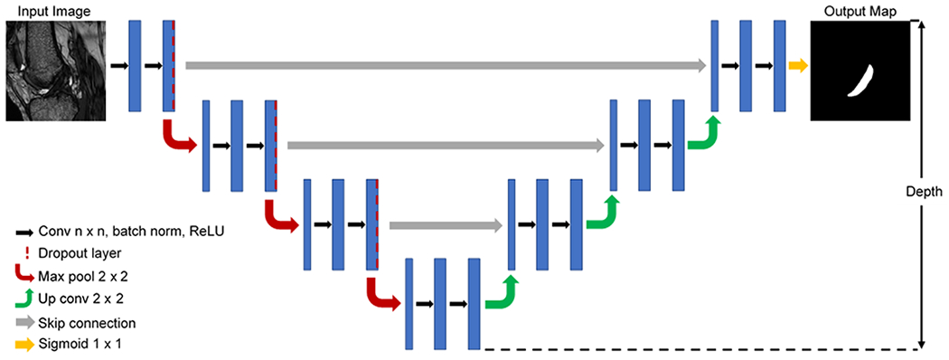
Example modified 2D U-Net architecture (note: final model depth was tuned as hyperparameter).

Bayesian optimization was employed for hyperparameter tuning, which uses an acquisition function (a Gaussian process) to determine where to search the hyperparameter space next in each iteration. This method is less computationally expensive than grid search, and by systematically incorporating knowledge of previous hyperparameter configurations into the search process, it often converges on an optimal solution more rapidly than random search.³³

The following hyperparameters were tuned with Bayesian optimization: filter sizes, kernel size, alpha (i.e. ReLU leakiness), dropout probability, and learning rate. Additionally, model depth, batch size, and use of batch normalization or local response normalization were tuned by manual search. A summary of the hyperparameter search space can be found in Table 1. Each MR image slice was treated as a single sample. Training samples were randomly shuffled, which improved training time without affecting performance. Model training was terminated if validation loss plateaued for 10 epochs to prevent overfitting and to reduce training time.

Table 1.

Hyperparameter search space for Bayesian optimization.

Hyperparameter	Values
Model Depth	[3, 4, 5]
Batch Size	[10, 20, 32]
Normalization Method	[Batch, Local Response, None]
Filter Sizes	[[16, 32, 64, 32, 16], [32, 64, 128, 64, 32], [64, 128, 256,128, 64], [16, 32, 64, 128, 64, 32, 16], [32, 64, 128, 256, 128, 64, 32], [64, 128, 256, 512, 256, 128, 64], [16, 32, 64, 128, 256, 128, 64, 32, 16], [32, 64, 128, 256, 512, 256, 128, 64, 32], [64, 128, 256, 512, 1024, 512, 256, 128, 64]]
Kernel Size	[3x3, 5x5, 7x7]
Alpha	[0, 0.1, 0.2, 0.3, 0.4, 0.5]
Dropout	[0, 0.1, 0.2, 0.3, 0.4, 0.5]
Learning Rate	[1e-3, 1e-4, 1e-5, 1e-3:1e-5 (variable; patience=5)]

The model was trained on a Dell Precision 3630 desktop (Dell Inc.; Round Rock, TX, USA) outfitted with an NVIDIA GeForce GTX 1080 GPU (NVIDIA Corporation; Santa Clara, CA, USA). Dice coefficient with Laplacian smoothing loss (Eq. 1) was used to address the class imbalance between the ratio of ACL to non-ACL voxels. The addition of a Laplacian smoothing coefficient of 1 in the numerator and denominator is necessary for the Dice coefficient loss to be continuously differentiable. A negative sign is also required as loss must be minimized but Dice coefficient maximized. Adaptive moment estimation (Adam)³⁴ was used as an optimizer during model training.

$${\text{Dice coefficient}}_{\text{LOSS}}=-\frac{2\mid y_{\text{true}}\bigcap y_{\mathit{pred}}\mid +1}{\mid y_{\text{true}}\mid +\mid y_{\mathit{pred}}\mid +1}$$ [1]

Test set probability outputs were thresholded for binary predictions. Probabilities greater than 0.5 were classified as ACL, and less than or equal to 0.5 as non-ACL. Test set slice predictions were merged by subject for final performance metric calculations.

Performance

The anatomical similarity of automatic segmentation relative to manual ground truth was assessed with Dice coefficient (Eq. 2), sensitivity (Eq. 3), and precision (Eq. 4). Dice coefficient measures the degree of similarity between the automatic and manual (ground truth) segmentations (TP = true positive, FP = false positive, FN = false negative). Sensitivity is the fraction of true positives that were correctly classified. Precision is the fraction of true positives out of all positive classifications. Greater Dice coefficient, sensitivity, and precision values indicate better segmentation performance relative to ground truth.

$$\text{Dice coefficient}=\frac{2\mathit{TP}}{\mathit{FP}+2\mathit{TP}+\mathit{FN}}$$ [2]

$$\text{Sensitivity}=\frac{\mathit{TP}}{\mathit{TP}+\mathit{FN}}$$ [3]

$$\text{Precision}=\frac{\mathit{TP}}{\mathit{TP}+\mathit{FP}}$$ [4]

For any automatic segmentation method to be effective for use in qMRI pipelines, quantitative features extracted from the automatic segmentations must be equivalent to those extracted from manual segmentation. Therefore, the median standardized signal intensity and ligament volume of the automated test set segmentations were assessed relative to the ground truth segmenter. Statistical significance of disagreements between the automated segmentation and ground truth were assessed using Wilcoxon signed rank tests (alpha=.05).

To assess the reproducibility of anatomical segmentation and subsequent quantitative measures, a randomly selected and anonymized subset of 10 test set MR imaging scans was segmented by two more segmenters, one with 6 months of experience and another with 2 years of experience segmenting ACLs. The ground truth segmenter also re-segmented this subset to evaluate re-test performance. Re-segmentations of the ground truth segmenter were completed on average 2.2 years after the initial segmentation. Anatomical similarity relative to ground truth was again evaluated by Dice coefficient, sensitivity, and precision. Median standardized signal intensity and volume of the ACL were calculated for each segmentation. Repeated measures analysis of variance (RANOVA) with pairwise Tukey Honest Significant Difference testing were used to assess the significance of differences on this subset (alpha=.05). All statistical analyses were performed in Python with the SciPy³⁵ and statsmodels³⁶ packages.

RESULTS

The optimized model utilized a deep architecture, with small batch size, medium kernel size, larger filter sizes, batch normalization, standard ReLU activation (i.e. alpha=0), high dropout probability in the downwards path, and a variable learning rate conditioned on validation loss (Table 2). The test set segmentation predictions of the final model configuration were anatomically similar to the ground truth, with per subject median Dice coefficient=.84, precision=.82, and sensitivity=.85 (Figure 2). Examples of raw MR images with corresponding ground truth manual segmentation and predicted automatic segmentation are shown in Figure 3. Qualitatively, some regions of disagreement were observed around the origin and insertion in some subjects (Figure 4). The typical mode of disagreement was the model leaving a slice unsegmented, where the ground truth segmenter did not. However, these regions were small relative to the total ligament.

Table 2.

Summary of optimal hyperparameters for final model configuration.

Hyperparameter	Value
Model Depth	5
Batch Size	10
Normalization Method	Batch
Filter Sizes	[64, 128, 256, 512, 1024, 512, 256, 128, 64]
Kernel Size	5x5
Alpha	0
Dropout	0.5
Learning Rate	1e-3:1e-5 (variable; patience=5)

Figure 2.

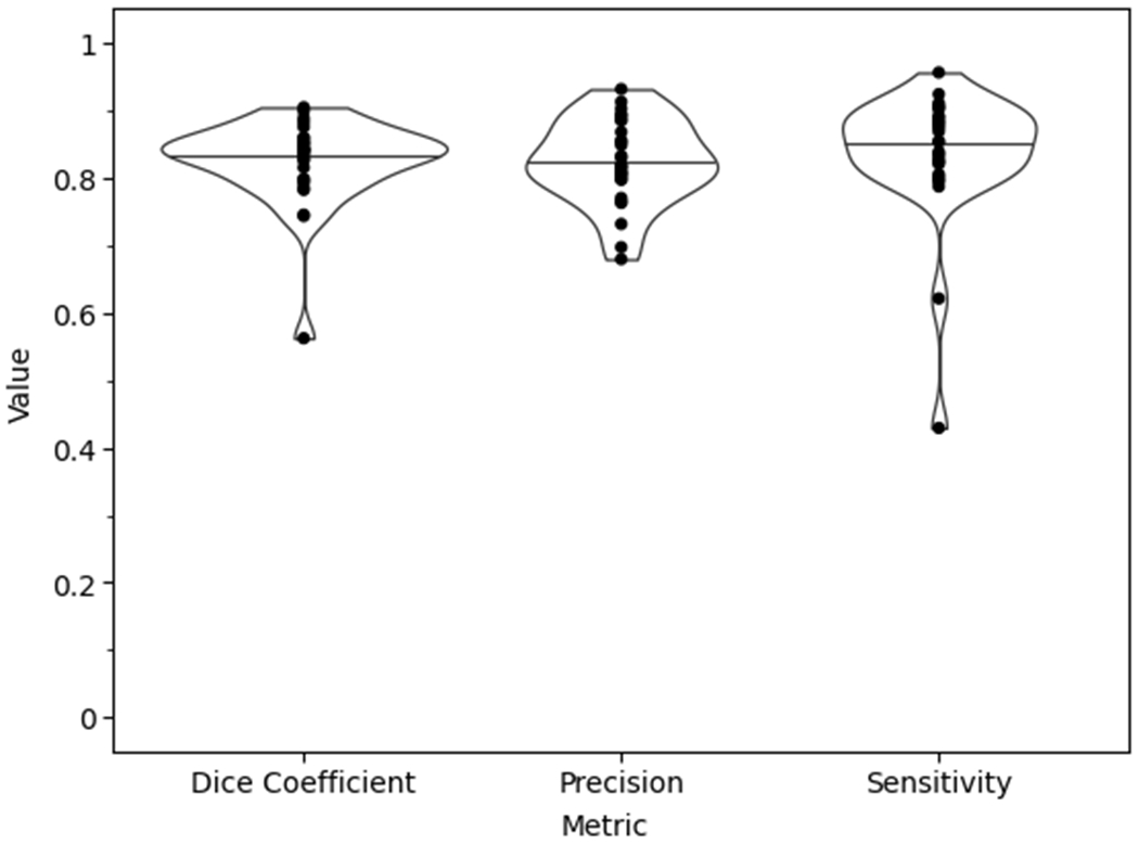
Final model test set performance violin plot with the data points superimposed of the anatomical similarity metrics.

Figure 3.

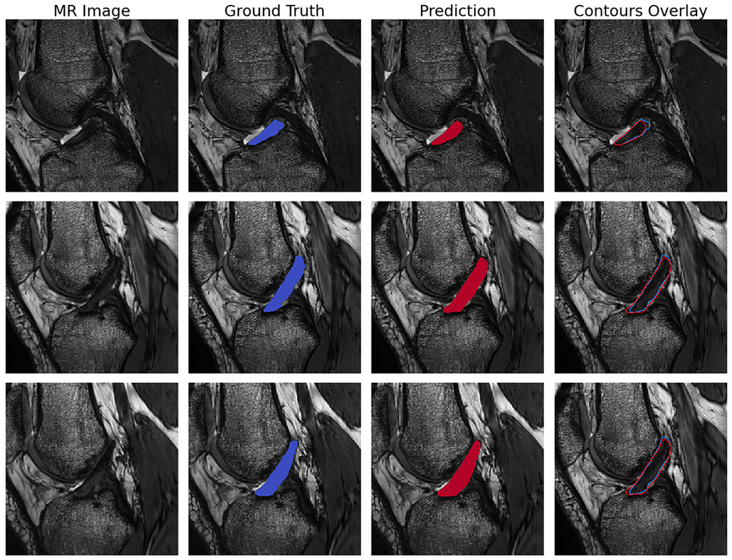
Example sagittal CISS slice segmentations from the final model predictions on randomly selected test set subjects. Each row is the same slice. Shown are the unsegmented slice (MR Image), ground truth manual segmentation (Ground Truth), automatic segmentation prediction (Prediction), and an overlay of manual and predicted segmentations (Contours Overlay).

Figure 4.

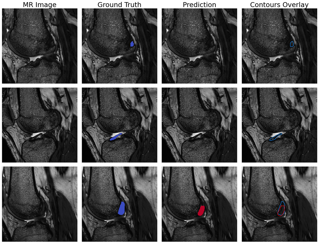
Example sagittal CISS slice segmentations showing areas of disagreement between the model predictions and ground truth. Each row is the same slice. Shown are the unsegmented slice (MR Image), ground truth manual segmentation (Ground Truth), automatic segmentation prediction (Prediction), and an overlay of manual and predicted segmentations (Contours Overlay).

Paired comparisons of median standardized signal intensity and volume showed differences of 0.3% (p=.9) and 2.3% (p=.08), respectively, between ground truth and the final model (Figure 5). Neither of these differences were statistically significant.

Figure 5.

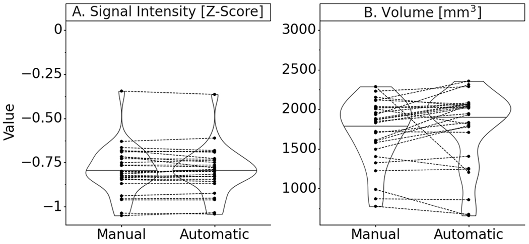
Final model test set performance violin plot with paired data points of the quantitative measures taken from ground truth manual segmentation and predicted automatic segmentation masks (Note: signal intensities are standardized by z-scoring for each image volume; Paired data points represent results on the same MRI scan; Summary statistics in Appendix 1).

On the random subset of test subjects, the deep learning model outperformed two additional manual segmenters relative to the ground truth segmenter in terms of Dice coefficient and sensitivity (Figure 6). However, the increase in Dice coefficient was only significantly different relative to Segmenter A (p=.001). The model performed as well as the manual segmenters with respect to precision. The model scored significantly higher on sensitivity than either manual segmenter (p=.001, p=.003). The model performed equally well to re-segmentation by the ground truth segmenter on all performance measures, when there was a 2.2 year interval between the original and re-test manual segmentations. The sensitivity of the model was greater than re-segmentation by the ground truth segmenter, though this finding was not a significant difference.

Figure 6.

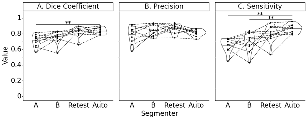
Test subset performance violin plot with paired data points on anatomical similarity metrics of manual segmenters (A, B), ground truth segmenter re-segmentation (Retest), and final automatic segmentation model (Note: * indicates P<.05; ** indicates P<.005; Paired data points represent performance on the same MRI scan; Summary statistics in Appendix 1).

Median standardized signal intensities were not significantly different across segmenters, with the exception of segmenter A, where the signal intensity was increased (Figure 7). However, no significant difference was detected. There were greater disagreements in volume between segmenters relative to ground truth than between automatic segmentation and ground truth. All manual segmentions, including the re-test segmentations of the ground truth segmenter, reported lower ligament volumes than the ground truth. The predicted segmentations of the model on this subset were larger in volume than the ground truth. Once again, these differences were not found to be significantly different.

Figure 7.

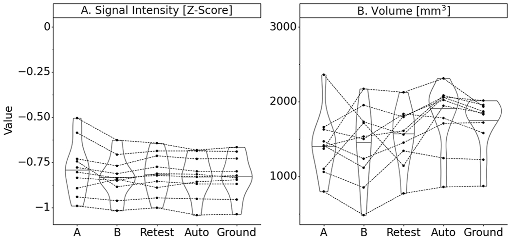
Test subset performance violin plot with paired data points on quantitative measures derived from segmentation masks of manual segmenters (A, B), ground truth segmenter re-segmentation (Retest), and final automatic segmentation model (Note: signal intensities are standardized by z-scoring for each image volume; Paired data points represent performance on the same MRI scan; Summary statistics in Appendix 1).

DISCUSSION

The goal of the current study was to validate an automated segmentation method for the ACL, that could replace manual segmentation in qMRI processing pipelines. We hypothesized that: a) a fully convolutional neural network could generate segmentations similar to manual segmentation both anatomically and on the basis of quantitative features (i.e. signal intensity and volume), and b) that the proposed deep learning model would be more reproducible than manual segmentation. Although there are many quantitative features of interest that may be measured after segmentation, including cross-sectional area, ligament length, and orientation (data presented in Appendix 2), for the current study signal intensity and volume of the ACL were the focus because they are currently used in downstream qMRI prediction models, such as for ACL failure load.¹⁴

On the full image test set, the automatic segmentation model scored highly on anatomical performance metrics. Furthermore, on a randomly selected subset of test subjects, the model’s predicted segmentations demonstrated greater anatomical similarity to ground truth than two manual segmenters in terms of Dice coefficient and sensitivity relative to ground truth, while showing similar precision. On these performance metrics, the model performed as well as re-segmentation by the ground truth segmenter.

Qualitatively, we observed greater variability at the origin and insertion of the ACL, for both the model and human segmenters relative to ground truth. As previously noted, prior attempts to semi-automatically segment the ACL faced difficulties at the origin and insertion.^{21; 22} However, a sub-regional analysis of the origin, insertion, and mid-substance only found a statistically significant decrease in automatic segmentation performance at the origin. No statistically significant difference was observed at the insertion, which demonstrated moderately higher performance (Appendix 3).

Nevertheless, the fully automated deep learning model achieved overall greater anatomical agreement relative to ground truth manual segmentation than these prior semi-automatic methods. Ho et al. reported a Dice coefficient of 0.38 and sensitivity of 0.43 for a semi-automated method using morphological operations and active contour (precision not reported).²¹ The graph cuts with patient-specific shape constraints method proposed by Lee et al. achieved a Dice coefficient of 0.66 (sensitivity and precision not reported).²² In contrast, the fully automated method proposed here achieved a Dice coefficient of 0.84, precision of 0.82, and sensitivity of 0.85.

The deep learning model yielded very similar median standardized signal intensity and volume measurements to ground truth on the test set, without any statistically significant differences. For use in qMRI pipelines, this is especially important, as a divergence in quantitative measurements could skew subsequent predictions of ACL mechanical properties and tissue health.¹⁴

Interestingly, in the randomized test subset, there was greater disagreement between manually segmented ligament volumes relative to ground truth, though this difference was not significant. It is likely that at least part of this disagreement is due to experience, as Segmenter A (6 months of experience) diverged to the greatest extent, followed by Segmenter B (2 years of experience). Yet, re-segmentation by the ground truth segmenter (greater than 5 years’ experience) still yielded differences in volume. These results highlight how the learning curve for manual segmentation is an obstacle for scaling up qMRI pipelines, and even then inter-segmenter or intra-segmenter variability is an inherent issue.

In contrast, the trained automatic segmentation model produces nearly identical segmentations on the same MR image, unlike a human segmenter. This is because no updates to the network’s weights and biases occur after training. Therefore, when predicting segmentation on the same MR image, the same series of operations will occur along the forward pass, with the only source of infinitesimal variation in such a case being machine error. By eliminating inter- and intra-segmenter variability, automatic segmentation removes a source of variation that would negatively affect downstream qMRI prediction models (e.g. for ACL failure load prediction).¹⁴

Another advantage of the deep learning model is that it is extremely fast at automatic segmentation. On the test set, mean segmentation time was 0.33 seconds per subject. In contrast, it has been our experience that manually segmenting the ACL from a CISS scan of the knee takes 1-2 hours. This major increase in efficiency overcomes another current preprocessing bottleneck that manual segmentation creates in MRI data pipelines.

The strength of this study is that it leverages a large dataset of intact ACL CISS MR scans with relatively high spatial resolution and contrast, from a cohort of patients relevant to the ACL-injured population. Since measures of signal intensity and volume obtained from CISS scans have been correlated to ACL mechanical properties,¹⁴ automatic segmentations from this sequence may be immediately useful for making quantitative predictions. Furthermore, because of the high contrast in these scans, the CISS sequence is useful for training a model that may then be transferred via transfer learning to other, lower resolution sequences such as T₂*.^{3; 12} Transferring the model to other sequences is the subject of ongoing work.

Given the positive results of the automatic deep learning model for segmenting the ACL, future work will focus on translating this trained model to lower resolution qMRI sequences, as well as other MRI sequences that are routinely used for clinical assessment (e.g. PD-SPACE). It is unlikely that this model will work well “off the shelf” with other MRI sequences, due to differences in acquisition parameters. However, translating the current model to other sequences may be accomplished using transfer learning.³⁷ In addition, this model was trained on intact ligaments. To be clinically useful, this model must also robustly segment ACL reconstruction grafts and repairs. This is also a task that may be accomplished by transfer learning, now that this validation with intact ligaments has been performed.

In conclusion, the proposed model segmented the ACL with greater speed and reliability than manual segmentation and may be scaled up without the lengthy training process associated with manual segmentation. This automated method may enable increased usage of qMRI in clinical trials for direct assessments of ligament outcomes by overcoming the segmentation time and expertise bottlenecks of manual processing following ACL injury or ACL surgery.

REFERENCES

- 1.Koff MF, Shah P, Pownder S, et al. 2013. Correlation of meniscal T2* with multiphoton microscopy, and change of articular cartilage T2 in an ovine model of meniscal repair. Osteoarthritis Cartilage 21:1083–1091. [DOI] [PMC free article] [PubMed] [Google Scholar]
- 2.Beveridge JE, Proffen BL, Karamchedu NP, et al. 2019. Cartilage damage is related to ACL stiffness in a porcine model of ACL repair. J Orthop Res 10:2249–2257. [DOI] [PMC free article] [PubMed] [Google Scholar]
- 3.Biercevicz AM, Murray MM, Walsh EG, et al. 2014. T2* MR relaxometry and ligament volume are associated with the structural properties of the healing ACL. J Orthop Res 32:492–499. [DOI] [PMC free article] [PubMed] [Google Scholar]
- 4.Biercevicz AM, Proffen BL, Murray MM, et al. 2015. T2* relaxometry and volume predict semi-quantitative histological scoring of an ACL bridge-enhanced primary repair in a porcine model. J Orthop Res 33:1180–1187. [DOI] [PMC free article] [PubMed] [Google Scholar]
- 5.Chu CR, Williams AA, West RV, et al. 2014. Quantitative magnetic resonance imaging UTE-T2* mapping of cartilage and meniscus healing after anatomic anterior cruciate ligament reconstruction. Am J Sports Med 42:1847–1856. [DOI] [PMC free article] [PubMed] [Google Scholar]
- 6.Williams A, Qian Y, Golla S, et al. 2012. UTE-T2* mapping detects sub-clinical meniscus injury after anterior cruciate ligament tear. Osteoarthritis Cartilage 20:486–494. [DOI] [PMC free article] [PubMed] [Google Scholar]
- 7.Williams AA, Titchenal MR, Andriacchi TP, et al. 2018. MRI UTE-T2* profile characteristics correlate to walking mechanics and patient reported outcomes 2 years after ACL reconstruction. Osteoarthritis Cartilage 26:569–579. [DOI] [PMC free article] [PubMed] [Google Scholar]
- 8.Titchenal MR, Williams AA, Chehab EF, et al. 2018. Cartilage subsurface changes to magnetic resonance imaging UTE-T2* 2 years after anterior cruciate ligament reconstruction correlate with walking mechanics associated with knee osteoarthritis. Am J Sports Med 46:565–572. [DOI] [PMC free article] [PubMed] [Google Scholar]
- 9.Pedoia V, Li X, Su F, et al. 2016. Fully automatic analysis of the knee articular cartilage T1ρ relaxation time using voxel-based relaxometry. J Magn Reson Imaging 43:970–980. [DOI] [PMC free article] [PubMed] [Google Scholar]
- 10.Chen M, Qiu L, Shen S, et al. 2017. The influences of walking, running and stair activity on knee articular cartilage: Quantitative MRI using T1 rho and T2 mapping. PLoS One 12:e0187008. [DOI] [PMC free article] [PubMed] [Google Scholar]
- 11.Knox J, Pedoia V, Wang A, et al. 2018. Longitudinal changes in MR T1ρ/T2 signal of meniscus and its association with cartilage T1p/T2 in ACL-injured patients. Osteoarthritis Cartilage 26:689–696. [DOI] [PMC free article] [PubMed] [Google Scholar]
- 12.Beveridge JE, Machan JT, Walsh EG, et al. 2018. Magnetic resonance measurements of tissue quantity and quality using T2* relaxometry predict temporal changes in the biomechanical properties of the healing ACL. J Orthop Res 36:1701–1709. [DOI] [PMC free article] [PubMed] [Google Scholar]
- 13.Pauli C, Bae WC, Lee M, et al. 2012. Ultrashort–echo time MR imaging of the patella with bicomponent analysis: correlation with histopathologic and polarized light microscopic findings. Radiology 264:484–493. [DOI] [PMC free article] [PubMed] [Google Scholar]
- 14.Biercevicz AM, Miranda DL, Machan JT, et al. 2013. In Situ, noninvasive, T2*-weighted MRI-derived parameters predict ex vivo structural properties of an anterior cruciate ligament reconstruction or bioenhanced primary repair in a porcine model. Am J Sports Med 41:560–566. [DOI] [PMC free article] [PubMed] [Google Scholar]
- 15.Kiapour AM, Fleming BC, Murray MM. 2017. Structural and anatomic restoration of the anterior cruciate ligament is associated with less cartilage damage 1 year after surgery: healing ligament properties affect cartilage damage. Orthop J Sports Med 5:2325967117723886. [DOI] [PMC free article] [PubMed] [Google Scholar]
- 16.Dam EB, Lillholm M, Marques J, et al. 2015. Automatic segmentation of high- and low-field knee MRIs using knee image quantification with data from the osteoarthritis initiative. J Med Imaging (Bellingham) 2:024001. [DOI] [PMC free article] [PubMed] [Google Scholar]
- 17.Gaj S, Yang M, Nakamura K, et al. 2019. Automated cartilage and meniscus segmentation of knee MRI with conditional generative adversarial networks. Magn Reson Med 84:437–449. [DOI] [PubMed] [Google Scholar]
- 18.Norman B, Pedoia V, Majumdar S. 2018. Use of 2D U-Net convolutional neural networks for automated cartilage and meniscus segmentation of knee MR imaging data to determine relaxometry and morphometry. Radiology 288:177–185. [DOI] [PMC free article] [PubMed] [Google Scholar]
- 19.Ahn C, Bui TD, Lee Y-W, et al. 2016. Fully automated, level set-based segmentation for knee MRIs using an adaptive force function and template: data from the osteoarthritis initiative. Biomed Eng Online 15. [DOI] [PMC free article] [PubMed] [Google Scholar]
- 20.Kashyap S, Oguz I, Zhang H, et al. 2016. Automated segmentation of knee MRI using hierarchical classifiers and just enough interaction based learning: data from osteoarthritis initiative. Springer International Publishing; pp. 344–351. [DOI] [PMC free article] [PubMed] [Google Scholar]
- 21.Ho JH, Lung WZ, Seah CL, et al. Anterior cruciate ligament segmentation: using morphological operations with active contour. 2010 4th International Conference on Bioinformatics and Biomedical Engineering. Chengdu: IEEE; pp. 1–4. [Google Scholar]
- 22.Lee H, Hong H, Kim J. 2014. Segmentation of anterior cruciate ligament in knee MR images using graph cuts with patient-specific shape constraints and label refinement. Comput Biol Med 55:1–10. [DOI] [PubMed] [Google Scholar]
- 23.Akkus Z, Galimzianova A, Hoogi A, et al. 2017. Deep learning for brain MRI segmentation: state of the art and future directions. J Digit Imaging 30:449–459. [DOI] [PMC free article] [PubMed] [Google Scholar]
- 24.Pereira S, Pinto A, Alves V, et al. 2016. Brain tumor segmentation using convolutional neural networks in MRI images. IEEE Trans Med Imaging 35:1240–1251. [DOI] [PubMed] [Google Scholar]
- 25.Kamnitsas K, Ledig C, Newcombe VFJ, et al. 2017. Efficient multi-scale 3D CNN with fully connected CRF for accurate brain lesion segmentation. Med Image Anal 36:61–78. [DOI] [PubMed] [Google Scholar]
- 26.Zhang W, Li R, Deng H, et al. 2015. Deep convolutional neural networks for multi-modality isointense infant brain image segmentation. Neuroimage 108:214–224. [DOI] [PMC free article] [PubMed] [Google Scholar]
- 27.Ronneberger O, Fischer P, Brox T. 2015. U-Net: convolutional networks for biomedical image segmentation. Springer International Publishing; pp. 234–241. [Google Scholar]
- 28.Murray MM, Kalish LA, Fleming BC, et al. 2019. Bridge-enhanced anterior cruciate ligament repair: two-year results of a first-in-human study. Orthop J Sports Med 7:2325967118824356. [DOI] [PMC free article] [PubMed] [Google Scholar]
- 29.Murray MM, Kiapour AM, Kalish LA, et al. 2019. Predictors of healing ligament size and magnetic resonance signal intensity at 6 months after bridge-enhanced anterior cruciate ligament repair. Am J Sports Med 47:1361–1369. [DOI] [PMC free article] [PubMed] [Google Scholar]
- 30.Murray MM, Fleming BC, Badger GJ, et al. 2020. Bridge-Enhanced Anterior Cruciate Ligament Repair Is Not Inferior to Autograft Anterior Cruciate Ligament Reconstruction at 2 Years: Results of a Prospective Randomized Clinical Trial. Am J Sports Med 48:1305–1315. [DOI] [PMC free article] [PubMed] [Google Scholar]
- 31.Abadi M, Agarwal A, Barham P, et al. 2015. TensorFlow: large-scale machine learning on heterogeneous distributed systems.
- 32.Chollet F 2015. Keras: the python deep learning library. GitHub. [Google Scholar]
- 33.O’Malley T, Bursztein E, Long J, et al. 2020. Keras Tuner. GitHub. [Google Scholar]
- 34.Kingma DP, Ba JL. 2017. Adam: a method for stochastic optimization. ArXiv. [Google Scholar]
- 35.Virtanen P, Gommers R, Oliphant TE, et al. 2020. SciPy 1.0: fundamental algorithms for scientific computing in Python. Nat Methods 17:261–272. [DOI] [PMC free article] [PubMed] [Google Scholar]
- 36.Skipper S, Josef P. 2010. Statsmodels: Econometric and Statistical Modeling with Python. The 9th Python in Science Conference. [Google Scholar]
- 37.Geron A 2019. Hands-On Machine Learning with Scikit-Learn, Keras & TensorFlow, 2nd ed: O’Reilly Media Inc.; 819 p. [Google Scholar]
Associated Data
This section collects any data citations, data availability statements, or supplementary materials included in this article.