A new mathematical model of COVID-19 using real data from Pakistan

Abstract

We propose a new mathematical model to investigate the recent outbreak of the coronavirus disease (COVID-19). The model is studied qualitatively using stability theory of differential equations and the basic reproductive number that represents an epidemic indicator is obtained from the largest eigenvalue of the next-generation matrix. The global asymptotic stability conditions for the disease free equilibrium are obtained. The real COVID-19 incidence data entries from 01 July, 2020 to 14 August, 2020 in the country of Pakistan are used for parameter estimation thereby getting fitted values for the biological parameters. Sensitivity analysis is performed in order to determine the most sensitive parameters in the proposed model. To view more features of the state variables in the proposed model, we perform numerical simulations by using different values of some essential parameters. Moreover, profiles of the reproduction number through contour plots have been biologically explained.

1. Introduction

COVID-19 is characterized as a disease caused by a novel COVID-19 now known as Severe Acute Respiratory Syndrome COVID-19 2 (SARS-CoV-2; formerly known as 2019-nCoV), first identified as a result of an outbreak of respiratory disease in Wuhan City, Hubei, China [1], [2], [3]. The report was initially made to the WHO on 31st December 2019. The WHO announced the COVID-19 outbreak as a global health concern on 30th January 2020 [4], [5]. COVID-19 is transmitted from human to human by direct contact with contaminated surfaces and by inhaling respiratory droplets from infected persons. Most infected people with the COVID-19 virus may develop mild or severe respiratory disease and recover without any special treatment being needed. Older people and those with underlying medical conditions such as cardiovascular disease, diabetes, chronic respiratory disease and cancer are more likely to experience serious illness.

COVID-19 can live for hours or days on a surface, due to factors such as sunlight, temperatures, and the type of surface. A person can get COVID-19 by touching a surface or object that has the virus on it and then touching their own mouth, nose, or eyes. However, this is not deemed to be the only way the virus spreads. Social distancing helps to minimize the chances of touching infected surfaces and contagious individuals outside the home [6]. There are currently no clear COVID-19 vaccines or medical treatments. There are, however, many ongoing clinical trials evaluating potential treatments. Governments implemented various control measures such as stringent and obligatory lock-downs, other measures such as social distancing, the avoidance of crowded meetings, the implementation of maximum numbers of people at every meeting and the use of face masks in order to effectively reduce COVID-19 transmission. Although the government has introduced a number of control initiatives. Contact tracing of reported infected cases has been stepped up across several nations to further help in curbing the spread of COVID-19, and confirmed cases are quickly put on isolation for proper care [7]. In Pakistan, the virus was first confirmed on 26th February 2020, when two cases were recorded, a student who just arrived from Iran and another person in the Islamabad Capital Territory. On 18th March, 2020, cases of COVID-19 have been recorded in all four provinces of Pakistan and Islamabad Capital Territory, and by 17th June, 2020 each district in Pakistan had recorded at least one confirmed case of COVID-19. As of October 10th, 2020, Pakistan had reported 324,077 cases of COVID-19, with 6673 deaths, 9384 active cases (undergoing treatment) and 308,020 recovered cases [8].

It is widely accepted that using mathematical models can predict the occurrence of infectious diseases. In this way, it is possible to find the likely outcome of an outbreak that is beneficial for the purposes of public health initiatives. By using compartmental models as a basic mathematical framework, the complex dynamics of epidemiological processes can be studied, as stated in [9]. Phenomenological expectations are the basis of the way these two populations interact and the models are thus constructed. To make up these models, ordinary differential equations (ODEs) have traditionally been investigated. Additionally, to make these models more functional, other populations, denoted by R, which is the picture of the immune/ removed/ recovered compartment, are also taken into account. A relevant point here is that, appropriate criteria for the specific disease under consideration should be obtained and that these criteria should be used to assess the effects of possible control steps, such as medication or vaccination. The problem, then, is how to incorporate such measures from an optimal point of view. Recently, many notable attempts have been made to implement various research for different types of integer compartmental model [10], [11], [12], [13], [14], [15]. Several mathematical models and non-mathematical findings have also been performed on COVID-19 as shown by most recent researchers in [16], [17], [18], [19], [20], [21], [22], [23], [24], [25], [26], [27], [28], [29], [30], [31].

This paper presents a deterministic mathematical model that assesses the impact of some control measures on the spread of COVID-19 in a human population; the study will focus on the situation in Pakistan, so real data from that country will be used. The model, parameterized using the total number of confirmed cases in COVID-19 and the number of active cases in Pakistan, would provide a reliable estimate of Pakistan’s disease burden. We hope that this study will give governments and public health sectors some insight into how to increase their non-pharmaceutical prevention initiatives to minimize the spread of the disease.

2. Formulation of the model

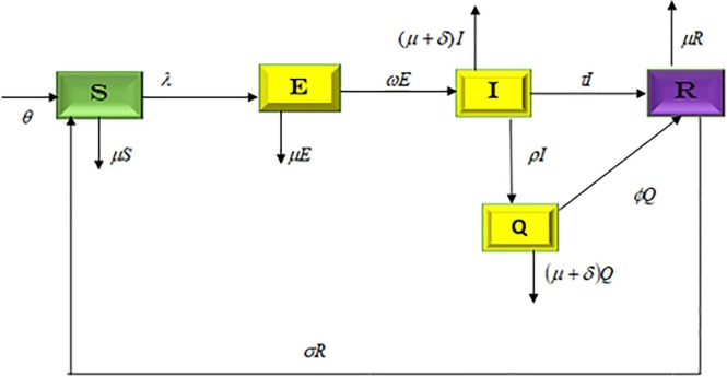
The model under consideration subdivides the population of human at time t into five compartments. That is, susceptible $S(t)$, exposed $E(t)$, infected $I(t)$, quarantine $Q(t)$ and recovered $R(t)$. We assumed that newborns can become infected with the virus that causes COVID-19 during childbirth or by exposure to sick caregivers after delivery. Therefore, the recruitment into the susceptible class is either by birth or immigration at a rate $\theta$. The progression of exposed individual to infected class is at a rate $\omega$. Individual in each of the classes can die a natural death at the rate $\mu$ . We also assumed that recovery from COVID-19 does not confers permanent immunity, therefore, the recovered individuals can returned back to susceptible class at a rate $\sigma$. The infected and quarantine individuals are reduced as a result of COVID-19 related complication at the rate $\delta$. $\tau$ and $\varphi$ represent the treatment rate for the infectious and quarantine individuals respectively. The force of infection $\lambda =\frac{{\alpha }_c(1-\psi )(1-\upsilon )(E+I)S}{N(t)}$ where $\psi$ is the proportion of individuals that maintain social distancing to prevent the spread of COVID-19 (at least two meter apart) this lies in the inequality $0⩽\psi ⩽1$. Also, $\upsilon$ represents fraction of the total population that effectively make use of the face mask and use of hand sanitizer. We assumed that face mask and use of hand sanitizer are highly effective when in public gathering so that $0⩽\upsilon ⩽1$.Thus, putting the above descriptions and assumptions together gives the following COVID-19 model, given by system of ordinary differential equations below as

$$\begin{array}{c}\frac{\mathit{dS}}{\mathit{dt}}=\theta -\frac{{\alpha }_c(1-\psi )(1-\upsilon )(E+I)S}{N(t)}-\mu S+\sigma R,\hfill \\ \frac{\mathit{dE}}{\mathit{dt}}=\frac{{\alpha }_c(1-\psi )(1-\upsilon )(E+I)S}{N(t)}-(\mu +\omega )E,\hfill \\ \frac{\mathit{dI}}{\mathit{dt}}=\omega E-(\mu +\delta +\rho +\tau )I,\hfill \\ \frac{\mathit{dQ}}{\mathit{dt}}=\rho I-(\mu +\delta +\varphi )Q,\hfill \\ \frac{\mathit{dR}}{\mathit{dt}}=\varphi Q+\tau I-(\sigma +\mu )R,\hfill \end{array}$$ (1)

where $\lambda =\frac{{\alpha }_c(1-\psi )(1-\upsilon )(E+I)S}{N(t)}$. The proposed model’s flowchart and parameters’ description are well explained in the Fig. 1 and the Table 1 , respectively.

Fig. 1.

Flow chart of the newly proposed COVID-19 model (1).

Table 1.

Detailed description of state variables and relevant parameters of the newly proposed COVID-19 model (1).

Variable	Description
$S(t)$	Susceptible class
$E(t)$	Exposed class
$I(t)$	Infected
$Q(t)$	Quarantine class
$R(t)$	Recovered class
$\theta$	Recruitment rate into susceptible population
$\mu$	Natural mortality rate
$\delta$	COVID-19 death rate
$\omega$	Progression rate from exposed to infectious class
$\sigma$	Rate of loss of immunity
$\tau$	Treatment rate for infectious individuals
$\varphi$	Treatment rate for quarantine individuals
$\psi$	Proportion of individuals that maintain social distancing
$\upsilon$	Usage of a face mask and hand sanitizer by a portion of the population
$\rho$	Rate of recovery from infection
${\alpha }_c$	Effective transmission rate

3. Model analysis

3.1. The invariant region

The invariant region defines the domain in which solutions to the model are of both biological and mathematical importance. All the variables and parameters of the model are assumed to be non-negative. To this end, we find first of all the total human population $M(t)$, where $M(t)=S(t)+E(t)+I(t)+Q(t)+R(t)$. By differentiating with respect to t on both side, we obtain the following:

$\frac{\mathit{dM}}{\mathit{dt}}=\frac{\mathit{dS}}{\mathit{dt}}+\frac{\mathit{dE}}{\mathit{dt}}+\frac{\mathit{dI}}{\mathit{dt}}+\frac{\mathit{dQ}}{\mathit{dt}}+\frac{\mathit{dR}}{\mathit{dt}}$. Upon simplification, we have $\frac{\mathit{dM}}{\mathit{dt}}=\theta -\mu (S+E+I+Q+R)-\delta I-\delta Q$. Therefore, $\frac{\mathit{dM}}{\mathit{dt}}=\theta -\mu N-\delta I-\delta Q$. In the absence of COVID-19 induced death ($\delta =0$), the above equation becomes

$$\frac{\mathit{dM}}{\mathit{dt}}=\theta -\mu M\text{.}$$ (2)

Integrating on both side of (2) yields the following

$${\int }_{}^{}\frac{\mathit{dM}}{\theta -\mu M}⩽{\int }_{}^{}\mathit{dt}\Rightarrow \frac{-1}{\mu }\ln \left(\theta -\mu M\right)⩽t+c\text{.}$$ (3)

This simplifies into,

$$\theta -\mu M⩾{\mathit{Be}}^{-\mu t},$$ (4)

with the initial condition $M(0)=M$ and B is a constant with the initial condition on eq. (4), we get the following

$$M_h⩽\frac{\theta }{\mu }-\left[\frac{\theta -\mu M_h}{\mu }\right]e^{-\mu t}\text{.}$$ (5)

As $t\to \infty$in eq. (5), we obtain

$$M_h⩽\frac{\theta }{\mu }\text{.}$$

Thus, the region in (6) is the feasible solution sets P for the total population in eq.(1).

$$P=\left\{(S,E,I,Q,R)\in {\mathbb{R}}_{+}^5:M⩽\frac{\theta }{\mu }\right\}\text{.}$$ (6)

Therefore, the proposed COVID-19 model (1) is well posed and are both epidemiologically and mathematically meaningful. It is therefore sufficient to examine the dynamics of the basic model in the domain P.

3.2. Basic reproduction ratio $({\mathcal{R}}_0)$

The basic reproductive ratio is a baseline measure in epidemiology that shows the total number of related diseases caused during an infectious period by a single infected person in a fully susceptible population. The matrices produced for the new disease and the condition for the disease transition are denoted by F and V. We have used the same strategy as described in [32].

$$\begin{array}{c}\mathcal{F}(X)=\left(\begin{array}{c}\hfill {\alpha }_c(1-\psi )(1-\upsilon )(E+I)S\hfill \\ \hfill \omega E\hfill \\ \hfill \rho I\hfill \end{array}\right)\text{.}\hfill \end{array}$$

$$\mathcal{V}(X)=\left(\begin{array}{c}\hfill (\mu +\omega )E\hfill \\ \hfill (\mu +\delta +\rho +\tau )I\hfill \\ \hfill (\mu +\delta +\varphi )Q\hfill \end{array}\right)\text{.}$$

The Jacobian matrix of $\mathcal{F}$ and $\mathcal{V}$ computed at the COVID-19 free equilibrium expressed as $\mathbf{F}$ and $\mathbf{V}$ such that,

$$\mathbf{F}=\left(\begin{array}{ccc}\hfill {\alpha }_c(1-\psi )(1-\upsilon )S\hfill & \hfill {\alpha }_c(1-\psi )(1-\upsilon )\hfill & \hfill 0\hfill \\ \hfill \omega \hfill & \hfill 0\hfill & \hfill 0\hfill \\ \hfill 0\hfill & \hfill \rho \hfill & \hfill 0\hfill \end{array}\right),$$

and

$$\mathbf{V}=\left(\begin{array}{ccc}\hfill \mu +\omega \hfill & \hfill 0\hfill & \hfill 0\hfill \\ \hfill 0\hfill & \hfill \mu +\delta +\rho +\tau \hfill & \hfill 0\hfill \\ \hfill 0\hfill & \hfill 0\hfill & \hfill \mu +\delta +\varphi \hfill \end{array}\right)\text{.}$$

$${\mathbf{V}}^{-\mathbf{1}}=\left(\begin{array}{ccc}\hfill \frac{1}{\mu +\omega }\hfill & \hfill 0\hfill & \hfill 0\hfill \\ \hfill 0\hfill & \hfill \frac{1}{\mu +\delta +\rho +\tau }\hfill & \hfill 0\hfill \\ \hfill 0\hfill & \hfill 0\hfill & \hfill \frac{1}{\mu +\delta +\varphi }\hfill \end{array}\right)\text{.}$$

The spectral radius of the matrix ${\mathbf{FV}}^{-\mathbf{1}}$ gives the basic reproduction number

$${\mathcal{R}}_0=\frac{{\alpha }_c\left(1-\psi \right)\left(1-\upsilon \right)\left(\mu +\delta +\rho +\tau +\omega \right)\theta }{\mu \left(\mu +\omega \right)\left(\mu +\delta +\rho +\tau \right)}\text{.}$$ (7)

3.3. Disease free equilibrium state and its global stability

The equilibrium state in the absence of COVID-19 is known as disease free equilibrium.This is obtained by equating the right hand side of Eq. (1) to zero. Thus, $E_0=(S,E,I,Q,R)=\left(\frac{\theta }{\mu },0,0,0,0\right)$ is found to be the COVID-19 free equilibrium state.

Theorem 3.1

If ${\mathcal{R}}_0⩽1$ then, in the absence of COVID-19, that is, the COVID-19 free equilibrium $E_0=\left(\frac{\theta }{\mu },0,0,0,0\right)$ is globally asymptotically stable. Otherwise, it is unstable.

Proof

Lyapunov function is commonly used to proof the Global Stability of the Disease Free Equilibrium [33], [34]. Consider the formed Lyapunov function of the type

$$\mathfrak{L}=a_{1}E+a_{2}I,$$

where $a_1=\left(\mu +\delta +\rho +\tau \right),a_2=\left(\mu +\omega \right)$. It is easy to establish that $a_1$ and $a_2$ are positive. Let’s differentiate $\mathfrak{L}$ with respect to time to have

$$\dot{\mathfrak{L}}=a_1\dot{E}+a_2\dot{I}\text{.}$$

$$\mathfrak{L}=(\mu +\delta +\rho +\tau +\omega )\left[{\alpha }_c(1-\psi )(1-\upsilon )(E+I)S-(\mu +\omega )E\right]+(\mu +\omega )\left[\omega E-(\mu +\delta +\rho +\tau )I\right]\text{.}$$ (8)

Solving eq.(8) to obtain

$$\dot{\mathfrak{L}}=\left[{\alpha }_c(1-\psi )(1-\upsilon )(\mu +\delta +\rho +\tau +\omega )S-(\mu +\omega )(\mu +\delta +\rho +\tau )\right](E+I)\text{.}$$ (9)

Simplifying eq.(8) with Eq. (9) to obtain

$$\dot{\mathfrak{L}}=(\mu +\omega )(\mu +\delta +\rho +\tau )\left[{\mathcal{R}}_0-1\right](E+I)\text{.}$$ (10)

We obtain from the eq.(10) that $\dot{\mathfrak{L}}=0$ when $E=I=0$ and ${\mathcal{R}}_0$. This means that the highest invariance set in $\left\{(S,E,I,Q,R)\in {\mathbb{R}}_{+}^5\right\}$ is the singleton DFE $(E_0)$ and by LaSalle’s Invariance Principle [35], DFE $(E_0)$ is globally asymptotically stable in ${\mathbb{R}}_{+}^5$.

4. Parameters fitting

The concept related with modeling a data set is ubiquitous almost in all applied areas of study. Making sure repetition of the data is an essential task because it would make predictions easier about items related to our data. In a curve fitting approach what we do is to take existing data and try to fit that data to a curve or a line. If we look at the data for fatalities or for number of cases or we look at the data for hospitalizations with respect to the coronavirus then we see from first row of the Table 2 that the curve has an upward trend from 01 July, 2020 to 14 August, 2020 in the country of Pakistan. Various approaches are available to adjust differential systems’ parameters to fit data so commonly we have a model of the system that might be something like an ordinary differential equation and then we also collect some data at particular time such as the one depicted by first rows in the Table 2. The table represents data versus model predictions along with absolute percentile errors wherein one can observe that the maximum error comes in second predicted value as about 11% whereas majority of errors are comparatively smaller. In this present section, we have used nonlinear curve fitting strategy to obtain unknown parameters of the proposed model (1) as listed in the Table 3 . The objective was to obtain smallest possible sum of squared residuals defined as:

$$\mathit{SSE}={\displaystyle \sum _{j=1}^n}{\left(x_j-k(t_j)\right)}^2,$$ (11)

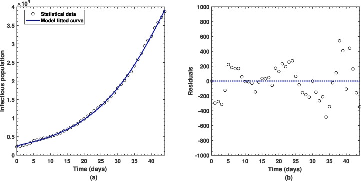
where $x_j$ and $k(t_j)$ stand for observational data values and predicted values from simulations of the infectious compartment in the model, respectively. Here, total number of data points are $n=45$ which demonstrate number of cases that occurred in Pakistan on a regular basis in Pakistan from 01 July, 2020 to 14 August, 2020. After achieving the objective of getting minimum error possible, we have obtained average absolute relative error to be equal to about $2.025841e-02$ which is considered to relatively small error whereas the basic reproductive number as shown in the Eq. (7) is computed as ${\mathcal{R}}_0\approx 4.8406e+00$ after using fitted parameters from Table 3. In addition to this, best fitting curve in comparison with the real observational data of COVID-19 cases is shown in the Fig. 2 wherein residuals have also been graphically depicted. One can observe from the plot how efficient the nonlinear least-squares curve fitting approach is in our model settings that ultimately helped to obtain unknown important parameters for validation of the proposed model of COVID-19 as shown by the Eq. (1).

Table 2.

Real cases for 45 days in 2020, Pakistan (http://covid.gov.pk/stats/pakistan): In each cell, first row stands for real cases, second row contains predicted values from the proposed system’s simulations for the infectious class and last row shows absolute percentile errors among observational data and the predicted values.

2289	2450	2708	2880	3287	3864	4070	4317	4598
2289	2.7466e+03	2.9841e+03	3.1944e+03	3.4114e+03	3.6418e+03	3.8874e+03	4.1494e+03	4.4289e+03
0	1.0799e+01	9.2525e+00	9.8414e+00	3.6473e+00	6.1015e+00	4.6974e+00	4.0393e+00	3.8183e+00
4784	5038	5374	5716	5985	6528	7016	7479	7993
4.7270e+03	5.0451e+03	5.3842e+03	5.7459e+03	6.1317e+03	6.5424e+03	6.9815e+03	7.4493e+03	7.9460e+03
1.2048e+00	1.4022e−01	1.9031e−01	5.1968e−01	2.3927e+00	2.2035e−01	4.9471e−01	3.9928e−01	5.9097e−01
8420	9216	9771	10513	11155	11940	12723	13328	14079
8.4769e+03	9.0424e+03	9.6422e+03	1.0281e+04	1.0962e+04	1.1685e+04	1.2450e+04	1.3265e+04	1.4129e+04
6.7067e−01	1.9204e+00	1.3360e+00	2.2557e+00	1.7614e+00	2.1853e+00	2.1925e+00	4.7809e−01	3.5248e−01
14885	15827	16817	18114	19103	20186	21501	22550	24073
1.5042e+04	1.6010e+04	1.7034e+04	1.8115e+04	1.9253e+04	2.0453e+04	2.1713e+04	2.3035e+04	2.4418e+04
1.0466e+00	1.1416e+00	1.2732e+00	4.0541e−03	7.8010e−01	1.3033e+00	9.7662e−01	2.1061e+00	1.4136e+00
25837	27474	29465	30941	32081	34336	35788	37218	38799
2.5861e+04	2.7363e+04	2.8924e+04	3.0533e+04	3.2189e+04	3.3894e+04	3.5625e+04	3.7377e+04	3.9147e+04
9.1520e−02	4.0706e−01	1.8711e+00	1.3371e+00	3.3536e−01	1.3050e+00	4.5695e−01	4.2501e−01	8.8829e−01

Table 3.

Best fitted parameters for the model.

Parameters	Interpretation	Value	Source
$\theta$	Recruitment rate into susceptible population	1.418243e−01	Fitted
$\mu$	Natural mortality rate	5.389301e−02	Fixed
$\delta$	COVID-19 death rate	6.839696e−01	Fitted
$\omega$	Progression rate from exposed to infectious class	2.421307e−02	fitted
$\sigma$	Immunity loss rate	2.104874e−01	Fitted
$\tau$	Treatment rate for infectious people	8.270934e−01	Fitted
$\varphi$	Treatment rate for people in quarantine	4.584931e−03	Fitted
$\psi$	Proportion of individuals that maintain social distancing	2.999373e−01	fitted
$\upsilon$	Proportion of the total population that effectively make use of the face mask and use of hand sanitizer	2.808803e−01	Fitted
$\rho$	Rate of recovery from infection	1.786530e−01	Fitted
${\alpha }_c$	Effective transmission rate	2.814715e−01	Fitted

Fig. 2.

(a) Best fitting of the proposed COVID-19 model with real statistical cases in Pakistan and the corresponding (b) residual plot.

5. Sensitivity of parameters

This section employs the principle of sensitivity analysis to investigate the robust significance of the standard parameters found in the unique specific reproduction number. Furthermore, with the aid of parameter values, both analytical and numerical values of the various parameters in ${\mathcal{R}}_0$ are determined from reliable assumptions. The analytical expressions obtained can be used to shed some light on how to track the onset of COVID-19 in different locations if the dynamics obey the model. ${\mathcal{R}}_0$ is a quantity that is considered the key means of minimizing and aborting the spread of victimization by decreasing the number to less than unity. The sensitivity index approach is used to calculate the model’s most sensitive parameters; those with non-negative signs are considered to be extremely and proportionally sensitive to increasing the value of Ro, while those with negative signs are less susceptible to lowering Ro, and the remaining category is neutrally sensitive (with zero relative sensitivity). The cause of raping transmission is widely understood to be directly correlated with the basic reproduction number ${\mathcal{R}}_0$. We measure the sensitivity indices for the state variables as follows:

$${\mathrm{\Upsilon }}_{{\mathbf{P}}_{\mathbf{i}}}^{{\mathbf{X}}_{\mathbf{i}}}=\frac{\partial {\mathbf{X}}_i}{\partial {\mathbf{P}}_i}\times \frac{{\mathbf{P}}_i}{{\mathbf{X}}_i},$$ (12)

where ${\mathbf{X}}_i$ represents the points at which the disease persist and ${\mathbf{P}}_i$ are the corresponding parameters in ${\mathbf{X}}_i$. In a similar way, the elasticity indices of the basic reproduction number to the associated parameters are described as:

$${\mathrm{\Upsilon }}_{{\mathbf{P}}_{\mathbf{i}}}^{{\mathcal{R}}_0}=\frac{\partial {\mathcal{R}}_0}{\partial {\mathbf{P}}_i}\times \frac{{\mathbf{P}}_i}{{\mathcal{R}}_0},$$ (13)

where ${\mathcal{R}}_0$ represents the basic reproduction number and ${\mathbf{P}}_i$ is as stated above. Thus, after some computation we reach:

$$\begin{array}{cc}\hfill & {\mathrm{\Upsilon }}_{{\alpha }_c}=1,\hfill \\ \hfill & {\mathrm{\Upsilon }}_{\theta }=1,\hfill \\ \hfill & {\mathrm{\Upsilon }}_{\psi }=-\frac{\psi }{1-\psi },\hfill \\ \hfill & {\mathrm{\Upsilon }}_{\upsilon }=-\frac{\upsilon }{1-\upsilon },\hfill \\ \hfill & {\mathrm{\Upsilon }}_{\delta }=\delta \mu \left(\mu +\omega \right)\left(\mu +\delta +\rho +\tau \right)\left(\frac{{\alpha }_c\left(1-\psi \right)\left(1-\upsilon \right)\theta }{\mu \left(\mu +\omega \right)\left(\mu +\delta +\rho +\tau \right)}-\frac{{\alpha }_c\left(1-\psi \right)\left(1-\upsilon \right)\left(\mu +\delta +\rho +\tau +\omega \right)\theta }{\mu \left(\mu +\omega \right){\left(\mu +\delta +\rho +\tau \right)}^2}\right)\hfill \\ \hfill & \times {\alpha }_c^{-1}{\left(1-\psi \right)}^{-1}{\left(1-\upsilon \right)}^{-1}{\left(\mu +\delta +\rho +\tau +\omega \right)}^{-1}{\theta }^{-1},\hfill \\ \hfill & {\mathrm{\Upsilon }}_{\rho }=\rho \mu \left(\mu +\omega \right)\left(\mu +\delta +\rho +\tau \right)\left(\frac{{\alpha }_c\left(1-\psi \right)\left(1-\upsilon \right)\theta }{\mu \left(\mu +\omega \right)\left(\mu +\delta +\rho +\tau \right)}-\frac{{\alpha }_c\left(1-\psi \right)\left(1-\upsilon \right)\left(\mu +\delta +\rho +\tau +\omega \right)\theta }{\mu \left(\mu +\omega \right){\left(\mu +\delta +\rho +\tau \right)}^2}\right)\hfill \\ \hfill & \times {\alpha }_c^{-1}{\left(1-\psi \right)}^{-1}{\left(1-\upsilon \right)}^{-1}{\left(\mu +\delta +\rho +\tau +\omega \right)}^{-1}{\theta }^{-1},\hfill \\ \hfill & {\mathrm{\Upsilon }}_{\tau }=\tau \mu \left(\mu +\omega \right)\left(\mu +\delta +\rho +\tau \right)\left(\frac{{\alpha }_c\left(1-\psi \right)\left(1-\upsilon \right)\theta }{\mu \left(\mu +\omega \right)\left(\mu +\delta +\rho +\tau \right)}-\frac{{\alpha }_c\left(1-\psi \right)\left(1-\upsilon \right)\left(\mu +\delta +\rho +\tau +\omega \right)\theta }{\mu \left(\mu +\omega \right){\left(\mu +\delta +\rho +\tau \right)}^2}\right)\hfill \\ \hfill & \times {\alpha }_c^{-1}{\left(1-\psi \right)}^{-1}{\left(1-\upsilon \right)}^{-1}{\left(\mu +\delta +\rho +\tau +\omega \right)}^{-1}{\theta }^{-1},\hfill \\ \hfill & {\mathrm{\Upsilon }}_{\omega }=\omega \mu \left(\mu +\omega \right)\left(\mu +\delta +\rho +\tau \right)\left(\frac{{\alpha }_c\left(1-\psi \right)\left(1-\upsilon \right)\theta }{\mu \left(\mu +\omega \right)\left(\mu +\delta +\rho +\tau \right)}-\frac{{\alpha }_c\left(1-\psi \right)\left(1-\upsilon \right)\left(\mu +\delta +\rho +\tau +\omega \right)\theta }{\mu {\left(\mu +\omega \right)}^2\left(\mu +\delta +\rho +\tau \right)}\right)\hfill \\ \hfill & \times {\alpha }_c^{-1}{\left(1-\psi \right)}^{-1}{\left(1-\upsilon \right)}^{-1}{\left(\mu +\delta +\rho +\tau +\omega \right)}^{-1}{\theta }^{-1}\text{.}\hfill \end{array}$$ (14)

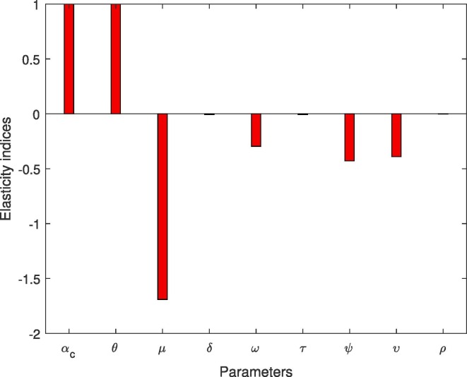
The numerical values showing the relative importance of the ${\mathcal{R}}_0$ parameters are shown in Table 4 . It can be shown that, based on the findings shown in Table 4, $\alpha c$ and $\theta$ have a clear effect on the virus’ stability and a very similar relationship. Therefore, by increasing $\alpha c$ and $\theta$ by $1\%,{\mathcal{R}}_0$ would have an increase of $1\%$ in influence. As shown in Table 4, there are parameters with a positive relation and those with a negative relation. A negative relationship suggests that an increase in the values of those metrics would help to mitigate the pandemic’s brutality. While a positive relationship indicates that the frequency of the pandemic en mass would be greatly influenced by an increase in the values of those parameters. The numerical signs in Table 4 are shown in the Fig. 3 . Fig. 3 depicts the powerful parameters that easily allow the virus to spread quickly.

Table 4.

The elasticity indices for ${\mathcal{R}}_0=4.840557333$ to the parameters of the model.

Parameters	Baseline value	Elasticity index
${\alpha }_c$	$2.814715e-01$	$+1.00000$
$\theta$	$1.418243e-01$	$+1.00000$
$\mu$	$5.389301e-02$	$-1.690420974$
$\delta$	$6.839696e-01$	$-0.5372779191e-2$
$\omega$	$2.421307e-02$	$-0.2963058176$
$\tau$	$8.270934e-01$	$-0.6497058068e-2$
$\psi$	$2.999373e-01$	$-0.4284434808$
$\upsilon$	$2.808803e-01$	$-0.3905890772$
$\rho$	$1.786530e-01$	$-0.1403371028e-2$

Fig. 3.

Normalized local sensitivity indices of ${\mathcal{R}}_0$ for each parameter.

6. Numerical dynamics

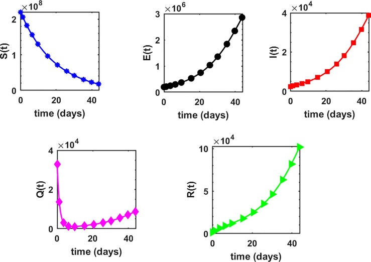
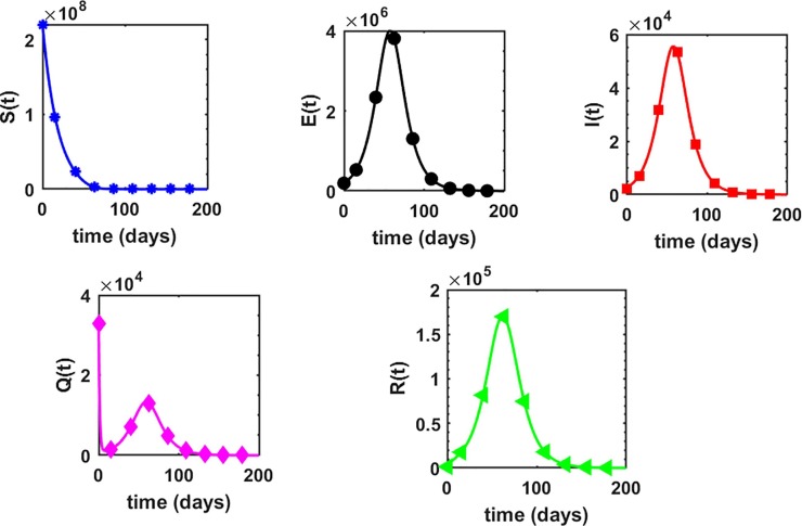
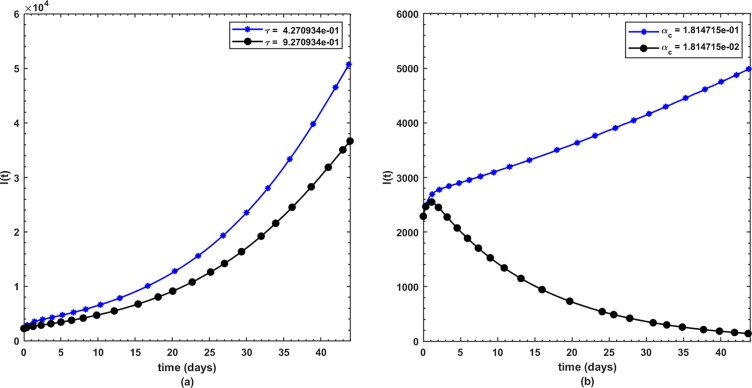
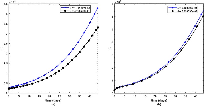
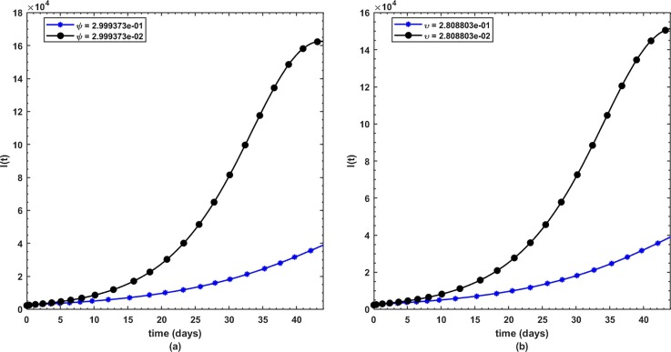
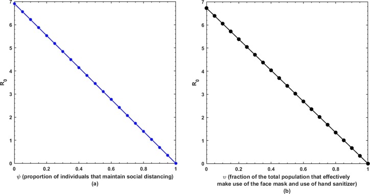
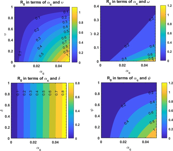
This is the position where we get deep insights into the complex behavior of the model. Under various computational simulations of the proposed model for state variables of interest, the transmission dynamics of an infectious disease can be adequately understood. In this section, we have conducted numerous simulations to understand the complex behavior of asymptomatically infectious individuals and the number of reproductive control ${\mathcal{R}}_0$. Various forms of time series graphs are shown by changing the parameter values under the parameters obtained by the nonlinear minimum-squares fitting approach in Section 5. Moreover, for the most significant parameters of the model, the dynamics of ${\mathcal{R}}_0$ are achieved through contour plots.The Susceptible $S(t)$, exposed $E(t)$, infected $I(t)$, quarantined $Q(t)$ and recovered $R(t)$ populations are investigated with different values of the parameters. As shown in Fig. 4, Fig. 5 over the interval [0 44], one can see that the $S(t)$ is decreasing, $E(t)$ is increasing, $I(t)$ is increasing, $Q(t)$ is decreasing with slight signal of an increase whereas the $R(t)$ is strictly increasing. By changing the interval to [0 200], the behavior of the aforementioned state variables changes with strong impact. Fig. 6 (a) depicts the dynamical behavior of the $I(t)$ with some values of the $\tau$ (treatment rate for infectious people) while Fig. 6(b) depicts the $I(t)$ individuals with some values of ${\alpha }_c$ (effective transmission rate). In Fig. 7 (a) and (b), $I(t)$ is plotted by varying $\rho$ (rate of recovery from infection) and $\delta$ (COVID-19 death rate), respectively. Moreover, the impact of $\psi$ (proportion of individuals that maintain social distancing) and $\upsilon$ (fraction of the total population that effectively Make use of the face mask and use of hand sanitizer) on the $I(t)$ individuals is depicted respectively in Fig. 8 (a) and (b). The profile of ${\mathcal{R}}_0$ versus some parameters via 2-dimentional and contour plots is shown in Fig. 9, Fig. 10 , respectively. Based on the illustrated figures, it can be noted that the methods used by the public health sector and the government concerned to resolve the situation leading to a rise in the pandemic would be more successful with a controlling transmission rate (see Fig. 5).

Fig. 4.

Profile of each state variable in the proposed COVID-19 model (1) over the time interval $[0,44]$.

Fig. 5.

(a) Profile of each state variable in the proposed COVID-19 model (1) over the time interval $[0,200]$.

Fig. 6.

(a) Dynamics of $I(t)$ under $\tau$ and (b) ${\alpha }_c$.

Fig. 7.

(a) Dynamics of $I(t)$ under $\rho$ and (b) $\delta$.

Fig. 8.

(a) Dynamics of $I(t)$ under $\psi$ and (b) $\upsilon$.

Fig. 9.

(a) Dependence of ${\mathcal{R}}_0$ on $\psi$ and on (b) $\upsilon$.

Fig. 10.

Dependence of ${\mathcal{R}}_0$ on different parameters of the COVID-19 model.

7. Conclusion

COVID-19 pandemic is one of the disturbing viruses that has confused the entire world. It has a subtle nature that causes delay of the emergence of its proper vaccine. Several measures and precautions by the concerned governments and medical practitioners have been suggested to combat the spread of the virus. One of the helpful ways to facilitate the understanding of the virus is the mathematical approach. In this regard, we proposed a new mathematical model on the disturbing contemporary pandemic called COVID-19 to comprehend its transmission dynamics. Several important properties of the new model such as the invariant region, equilibrium state, basic reproduction number, global stability of the free disease equilibrium have been investigated in the present research work. Moreover, real statistical data set from 01 July, 2020 to 14 August, 2020 in the country of Pakistan is also used to obtain best fitted values of some parameters using nonlinear least squares estimation technique with MATLAB function lsqcurvefit. Sensitivity analysis of the parameters has been conducted in order to determine the most sensitive parameters of the new proposed model. Numerical simulations confirmed these observations with best fitted curve obtained for the proposed model. In this research, it was shown that with a regulated transmission rate, the methods used by the public health sector and the government to address the situation leading to an increase in the pandemic will be more effective. Following the strategy employed in recently published researches [36], [37], [38], [39], [40], [41], [42], [43], [44], [45], the proposed COVID-19 model will be investigated in more detail in future research work.

Availability of data and material

All the data used in this manuscript can be found on WHO website.

Authors’ contributions

All authors have read and approved the final manuscript.

Funding

Not applicable.

Declaration of Competing Interest

The authors declare that they have no known competing financial interests or personal relationships that could have appeared to influence the work reported in this paper.

References

- 1.Rothana H.A., Byrareddy S.N. The epidemiology and pathogenesis of coronavirus disease (COVID-19) outbreak. J Autoimmun. 2020;109 doi: 10.1016/j.jaut.2020.102433. [DOI] [PMC free article] [PubMed] [Google Scholar]
- 2.Lu H. Drug treatment options for the 2019-new coronavirus (2019-nCoV) Biosci Trends. 2020 doi: 10.5582/bst.2020.01020. [DOI] [PubMed] [Google Scholar]
- 3.Bassetti M, Vena A, Giacobbe DR. The Novel Chinese coronavirus (2019-nCoV) infections: challenges for fighting the storm. Eur J Clin Invest 2020; e13209. doi.org/10.1111/eci.13209. [DOI] [PMC free article] [PubMed]
- 4.COVID-19 Coronavirus Pandemic. www.worldometers.info/coronavirus/#repro, Accessed July 20, 2020.
- 5.Wrapp D., Wang N., Corbett K. Cryo-EM structure of the 2019-nCoV spike in the prefusion conformation. Science. 2020;2:7–28. doi: 10.1126/science.abb2507. [DOI] [PMC free article] [PubMed] [Google Scholar]
- 6.Zhu N., Zhang D., Wang W. A novel coronavirus from patients with pneumonia in China, 2019. New England J Med. 2020;382:727–733. doi: 10.1056/NEJMoa2001017. [DOI] [PMC free article] [PubMed] [Google Scholar]
- 7.The Nigeria Center for Disease Control. https://covid19.ncdc.gov.ng; 2020.
- 8.World Health Organization. Coronavirus disease 2019 (COVID-19), Situation Report-80. https://www.who.int/docs/default-source/coronaviruse/situation-reports/20200409-sitrep-80-covid-19.pdf?sfvrsn=1b685d64-6. Published April 9, 2020. Accessed August 10th, 2020.
- 9.Rao F., Mandal P.S., Kang Y. Complicated endemics of an SIRS model with a generalized incidence under preventive vaccination and treatment controls. Appl Math Model. 2019;67:38–61. [Google Scholar]
- 10.Li L., Sun C., Jia J. Optimal control of a delayed SIRC epidemic model with saturated incidence rate. Optim Control Appl Met. 2018;40(2):367–374. [Google Scholar]
- 11.Acay B., Inc M., Khan A. Fractional methicillin-resistant Staphylococcus aureus infection model under Caputo operator. J Appl Math Comput. 2021 doi: 10.1007/s12190-021-01502-3. [DOI] [PMC free article] [PubMed] [Google Scholar]
- 12.Lin J., Xu R., Tian X. Global dynamics of an age-structured cholera model with both human-to-human and environment-to-human transmissions and saturation incidence. Appl Math Model. 2018;63:688–708. [Google Scholar]
- 13.Yusuf A., Acay B., Mustapha U.T., Inc M., Baleanu D. Mathematical modeling of pine wilt disease with Caputo fractional operator. Chaos Solitons Fract. 2021;143 [Google Scholar]
- 14.Ahmed I., Goufo E.F.D., Yusuf A., Kumam P., Chaipanya P., Nonlaopon K. An epidemic prediction from analysis of a combined HIV-COVID-19 co-infection model via ABC fractional operator. Alexand Eng J. 2021;60:2979–2995. [Google Scholar]
- 15.Kirtphaiboon S, Humphries U, Amir Khan, Yusuf A. Model of rice blast disease under tropical climate conditions. Chaos Solitons Fract 143: 2021; 110530.
- 16.Aguilar JB, Faust GSM, Westafer LM, Gutierrez JB. Investigating the impact of asymptomatic carriers on COVID-19 transmission. Preprint doi:10.1101/2020.03.18.20037994.
- 17.Musa S.S., Qureshi S., Zhao S., Yusuf A., Mustapha U.T., He D. Mathematical modeling of COVID-19 epidemic with effect of awareness programs. Infect Disease Model. 2021;6:448–460. doi: 10.1016/j.idm.2021.01.012. [DOI] [PMC free article] [PubMed] [Google Scholar]
- 18.Maier B.F., Brockmann D. Effective containment explains subexponential growth in recent confirmed COVID-19 cases in China. Science. 2020;08 doi: 10.1126/science.abb4557. [DOI] [PMC free article] [PubMed] [Google Scholar]
- 19.Ndaïrou F., Area I., Nieto J.J., Torres D.F.M. Mathematical modeling of COVID-19 transmission dynamics with a case study of Wuhan. Chaos Solitons Fract. 2020 doi: 10.1016/j.chaos.2020.109846. [DOI] [PMC free article] [PubMed] [Google Scholar]
- 20.Yang C, Wang J. A mathematical model for the novel coronavirus epidemic in Wuhan, China. Math Biosci Eng 17 (3): 2708–2724. [DOI] [PMC free article] [PubMed]
- 21.Fang Y., Nie Y., Penny M. Transmission dynamics of the covid-19 outbreak and effectiveness of government interventions: a data-driven analysis. J Med Virol. 2020;2:6–21. doi: 10.1002/jmv.25750. [DOI] [PMC free article] [PubMed] [Google Scholar]
- 22.Xinmiao R., Liu Y., Huidi C., Meng F. Effect of delay in diagnosis on transmission of COVID-19. Math Biosci Eng. 2020;17:2725. doi: 10.3934/mbe.2020149. (mbe-17-03-149) [DOI] [PubMed] [Google Scholar]
- 23.Mizumoto K., Chowell G. Estimating risk for death from 2019 novel coronavirus disease, China, January–February 2020. Emerg Infect Diseases. 2020;1:77–78. doi: 10.3201/eid2606.200233. [DOI] [PMC free article] [PubMed] [Google Scholar]
- 24.Hellewell J., Abbott S., Gimma A., Bosse N.I., Jarvis C.I., Russell T.W., Munday J.D., Kucharski A.J., Edmunds W.J., Sun F. Feasibility of controlling COVID-19 outbreaks by isolation of casesand contacts. Lancet Global Health. 2020 doi: 10.1016/S2214-109X(20)30074-7. [DOI] [PMC free article] [PubMed] [Google Scholar]
- 25.Okuonghae D., Omame A. Analysis of a mathematical model for COVID-19 population dynamics in Lagos, Nigeria. Chaos Solitons Fract. 2020 doi: 10.1016/j.chaos.2020.110032. [DOI] [PMC free article] [PubMed] [Google Scholar]
- 26.Liu Y., Gayle A.A., Wilder-Smith A., Rocklöv J. The reproductive number of COVID-19 is higher compared to SARS coronavirus. J Travel Med. 2020:1–4. doi: 10.1093/jtm/taaa021. [DOI] [PMC free article] [PubMed] [Google Scholar]
- 27.Li Y, Wang B, Peng R, Zhou C, Zhan Y, Liu Z, et al. Mathematical modeling and epidemic prediction of COVID-19 and its significance to epidemic prevention and control measures. Ann Infect Disease Epidemiol 2020; Ann Infect Dis Epidemiol 5(1):1052.
- 28.Chimmula V.K.R., Zhang L. Time series forecasting of COVID-19 transmission in Canada using LSTM networks. Chaos Solitons Fract. 2020;135 doi: 10.1016/j.chaos.2020.109864. [DOI] [PMC free article] [PubMed] [Google Scholar]
- 29.Naik P.A., Yavuz M., Qureshi S., Zu J., Townley S. Modeling and analysis of COVID-19 epidemics with treatment in fractional derivatives using real data from Pakistan. Eur Phys J Plus. 2020;135(10):1–42. doi: 10.1140/epjp/s13360-020-00819-5. [DOI] [PMC free article] [PubMed] [Google Scholar]
- 30.Jia J., Ding J., Liu S., Liao G., Li J., Duan B., Wang G., Zhang R. Modeling the control of COVID-19: impact of policy interventions and meteorological factors. Electron J Differ Equ. 2020;23:1–24. [Google Scholar]
- 31.Anastassopoulou C., Russo L., Tsakris A., Siettos C. Data-based analysis, modelling and forecasting of the COVID-19 outbreak. PLoS One. 2020;15(3):e0230405. doi: 10.1371/journal.pone.0230405. https://doi.org/10.1371/ journal.pone.0230405. [DOI] [PMC free article] [PubMed] [Google Scholar]
- 32.van den Driessche P., Watmough J. Reproduction numbers and sub-threshold endemic equilibria for compartmental models of disease transmission. Math Biosci. 2002;180:29–48. doi: 10.1016/s0025-5564(02)00108-6. [DOI] [PubMed] [Google Scholar]
- 33.Gashirai T.B., Musekwa-Hove S.D., Lolika P.O., Mushayabasa S. Global stability and optimal control analysis of a foot-and-mouth disease model with vaccine failure and environmental transmission? Chaos Solitons Fract. 2020;132 [Google Scholar]
- 34.Peter OJ, Viriyapong R, Oguntolu FA, Yosyingyong P, Edogbanya HO, Ajisope MO. Stability and optimal control analysis of an SCIR epidemic model. J Math.
- 35.La Salle J., Lefschetz S. SIAM; Philadelphia: 1976. The stability of dynamical systems. [Google Scholar]
- 36.Khana A., Zarina R., Hussain G. Stability analysis and optimal control of covid-19 with convex incidence rate in Khyber Pakhtunkhawa (Pakistan) Results Phys. 2021;20 doi: 10.1016/j.rinp.2020.103703. [DOI] [PMC free article] [PubMed] [Google Scholar]
- 37.Baba I.A., Yusuf A., Nisar K.S., Abdel-Atye A.H., Nofal F.T.A. Mathematical model to assess the imposition of lockdown during COVID-19 pandemic. Results Phys. 2021;20 doi: 10.1016/j.rinp.2020.103716. [DOI] [PMC free article] [PubMed] [Google Scholar]
- 38.Mahmoudi M.R., Baleanu D., Mansor Z., Tuan B.A., Pho K.H. Fuzzy clustering method to compare the spread rate of Covid-19 in the high risks countries. Chaos Solitons Fract. 2020;140 doi: 10.1016/j.chaos.2020.110230. [DOI] [PMC free article] [PubMed] [Google Scholar]
- 39.T.H. Zhao, O. Castillo, H. Jahanshah et al. A fuzzy-based strategy to suppress the novel coronavirus (2019-NCOV) massive outbreak. Appl Comput Math 20(N. 1): Special Issue, 2021; 160–176.
- 40.Inc M., Acay B., Berhe H.W. Analysis of novel fractional COVID-19 model with real-life data application. Results Phys. 2021;23 doi: 10.1016/j.rinp.2021.103968. [DOI] [PMC free article] [PubMed] [Google Scholar]
- 41.Ahmed I., Modu G.U., Yusuf A., Kumam P., Yusuf I. A mathematical model of Coronavirus Disease (COVID-19) containing asymptomatic and symptomatic classes. Results Phys. 2021;21 doi: 10.1016/j.rinp.2020.103776. [DOI] [PMC free article] [PubMed] [Google Scholar]
- 42.Peter, Shaikh OJ, Ibrahim AS, Nisar MO, Baleanu KS, Khan D, I, Abioye AI. Analysis and dynamics of fractional order mathematical model of COVID-19 in Nigeria using Atangana-Baleanu operator. CMC-Comput Mater Continua 66(2): 2021; 1823-1848.
- 43.Abioye A.I., Umoh M.D., Peter O.J., Edogbanya H.O., Oguntolu F.A., Kayode O., Amadiegwu S. Forecasting of COVID-19 pandemic in Nigeria using real statistical data. Commun Math Biol Neurosci. 2021 Article ID 2. [Google Scholar]
- 44.Attia N., Akgül A., Seba D., Nour A. An efficient numerical technique for a biological population model of fractional order. Chaos Solitons Fract Elsevier. 2020;141(C) [Google Scholar]
- 45.Ayub, Bashdar A, Mahmud S, Ali M, Sarbaz A, Khoshnaw HA. Analysis coronavirus disease (COVID-19) model using numerical approaches and logistic model. AIMS Bioeng 7 (3): 2020; 130–146. doi:10.3934/bioeng.2020013.
Associated Data
This section collects any data citations, data availability statements, or supplementary materials included in this article.
Data Availability Statement