Transmission analysis of COVID-19 with discrete time imported cases: Tianjin and Chongqing as cases

Abstract

In 2020, an unexpectedly large outbreak of the coronavirus disease 2019 (COVID-19) epidemic was reported in mainland China. As we known, the epidemic was caused by imported cases in other provinces of China except for Hubei in 2020. In this paper, we developed a differential equation model with tracing isolation strategy with close contacts of newly confirmed cases and discrete time imported cases, to perform assessment and risk analysis for COVID-19 outbreaks in Tianjin and Chongqing city. Firstly, the model behavior without imported cases was given. Then, the real-time regeneration number in Tianjin and Chongqing city revealed a trend of rapidly rising, and then falling fast. Finally, sensitivity analysis demonstrates that the earlier with Wuhan lock-down, the fewer cases in these two cities. One can obtain that the tracing isolation of close contacts of newly confirmed cases could effectively control the spread of the disease. But it is not sensitive for the more contact tracing isolation days on confirmed cases, the fewer cases. Our investigation model could be potentially helpful to provide model building technology for the transmission of COVID-19.

1. Introduction

Coronavirus disease 2019 (COVID-19) is an infectious disease caused by a newly discovered coronavirus, which is distinct from other existing types of coronavirus. According to the report by World Health Organization (WHO), most common symptoms are fever, dry cough and tiredness. Most people infected with the COVID-19 virus will experience mild to moderate respiratory illness and recover without requiring special treatment. At the beginning of 2020, COVID-19 was reported in Wuhan city, China (Li et al., 2020a). With the arrival of 2020 Spring Festival, massive travelling occurred from Wuhan to other parts of China, which contributed to the spread of COVID-19. On January 20, the Chinese government has revised the law provisions concerning infectious diseases and added the COVID-19 as Category B infectious disease. Public health officials have announced Category B infectious diseases are managed according to Category A, the same as SARS in 2003. In order to control the transmission of COVID-19, the Chinese authorities introduced the implementation of the lock-down strategy in Wuhan to shut down the movement on 23 January 2020. All provincial government initiated a first-level emergency response from 25 January 2020 (Chinese lunar new year). And some non-pharmaceutical interventions include strict controls on travel, the surveillance for newly confirmed cases, and the tracing and management with close contacts of newly confirmed cases, and the registered individuals with home quarantine for at least 14 days (Chinazzi et al., 2020; Li et al., 2020b). All of these measures are designed to early detection, early reporting and early quarantine for COVID-19.

Mathematical modeling has been influential in providing deeper understanding on the transmission mechanisms and burden of the ongoing COVID-19 pandemic, contributing to the development of public health policy and understanding. To our knowledge, some works have done research on transmission dynamics COVID-19 in mainland China (Chen et al., 2020; Du et al., 2020; Li et al., 2020b; Lin et al., 2020; Sun et al., 2020; Tang et al., 2020a, 2020b, 2020c; Wu et al., 2020; Yang et al., 2020). Li et al. (Li et al., 2020b) developed a SEIQR difference-equation model of COVID-19 in Shanxi province that takes into account the transmission with discrete time imported cases. Sun et al. (Sun et al., 2020) presented a dynamical model to show the propagation of COVID-19 in Wuhan and the effects of lock-down and medical resources. Tang et al. (Tang et al., 2020a, 2020b, 2020c) devised SEIR model on the estimation of the transmission risk of COVID-19 and showed the effectiveness of control strategy by intensive contact tracing followed by quarantine and isolation in mainland China. However, there is little work focused on the influence on contact tracing quarantine measures with the confirmed cases in some other provinces with discrete imported cases except Hubei Provinces in mainland China. Therefore, understanding the factors influencing COVID-19 outbreaks has become a major provincial public health priority in some provinces other than Hubei Province.

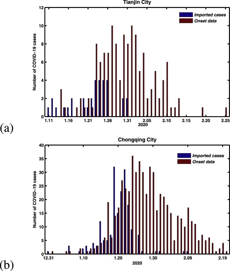
Using information published by the Health Commission of Tianjin and Chongqing city, we constructed a data-set of COVID-19 patients including these two cities. The detailed information includes the cumulative and daily laboratory-confirmed cases, and life track of these laboratory-confirmed cases. By means of statistical analysis the life track of all laboratory-confirmed cases, we obtain the data of symptom onset for all laboratory-confirmed cases, and arrival date of the confirmed COVID-19 cases in these two cities (we found that almost all confirmed cases arrived in these two cities without any symptoms). The newly onset of symptoms COVID-19 cases and the actual time of arrival in Tianjin and Chongqing City with confirmed COVID-19 cases were shown in Fig. 1. At the end of February, the cumulative confirmed cases and the imported cases of these two cities (Tianjin and Chongqing) were (136, 34) and (576, 187), respectively.

Fig. 1.

Time differences for between disease onset of symptoms and the arrival in these two cities with COVID-19 cases. (a) Tianjin City. (b) Chongqing City.

In this study, to make predictions and perform assessment and risk analysis for COVID-19 outbreaks in Tianjin and Chongqing city, we developed differential equation model with tracing isolation strategy with close contacts of newly confirmed cases and discrete time imported cases. The model behavior without imported cases was given. Finally, the real-time regeneration numbers in these two cities were given, the model parameters were estimated, and numerical simulations support the data reasonably well. From sensitivity analyses, one conclude that the tracing isolation of close contacts of newly confirmed cases can effectively control the spread of the disease.

2. Mathematical model

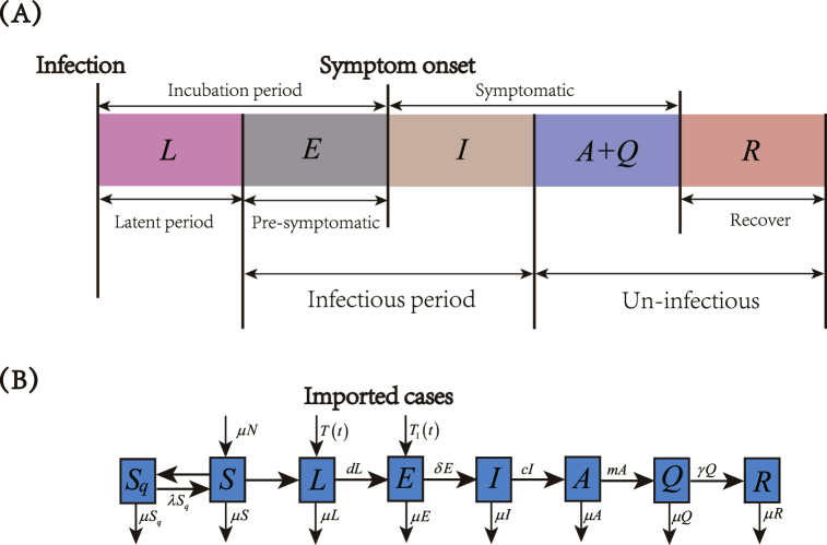
In this study, we developed a SLEIAQRS_q differential equation model with tracing isolation strategy for close contacts of newly confirmed cases to describe the transmission of COVID-19 in Tianjin and Chongqing City. Fig. 2 (A) shows the COVID-19 disease progression. An individual infected first goes through a non-infectious latent phase. Then followed by an infectious period that spans across symptom onset. In the pre-symptomatic phase, the person is infectious without symptoms. When the individual had the symptom onset, the person enters the symptomatic phase, and continues to be infectious. Hence, the model classified the human population (N(t)) into susceptible compartment S(t), latent compartment L(t), pre-symptomatic compartment E(t), symptomatic infectious compartment I(t), symptomatic un-infectious compartment A(t), confirmed compartment Q(t), recover compartment R(t) and quarantine susceptible compartment S_q(t). The period in incubation compartment is from time of infection to time of onset of symptoms, which includes the latent period L and the pre-symptomatic period E. Confirmed class Q(t) means the individual with laboratory-confirmed diagnosis. Once a individual is diagnosed in mainland China, who will be immediately arranged for hospitalization and isolation treatment, and will not participate in transmission.

Fig. 2.

(A) COVID-19 disease progression. (B) Transmission diagram of COVID-19.

Human population birth and death rates were assumed the same. The human host latent period and pre-symptomatic period were 1/d and 1/δ days, respectively. T(t) and T₁(t) were the imported COVID-19 cases at discrete time t, which were considered entering the latent compartment L(t) and pre-symptomatic compartment E, respectively. The transfer rate from symptomatic infectious cases to symptomatic un-infectious cases was c, symptomatic un-infectious cases at the rate m reverted to confirmed cases and the recover rate was γ. Susceptible humans acquired COVID-19 through direct contact with pre-symptomatic cases and symptomatic un-infectious cases at rates $\frac{\beta S(t)E(t)}{N(t)}$ and $\frac{{\beta }_{1}S(t)I(t)}{N(t)}$, respectively. In this study, the tracking isolation strategy for close contacts of newly confirmed cases was considered. Hence, the susceptible cases of tracing isolation was $\frac{bmS(t)A(t)}{N(t)}$ (b is the tracing isolation individuals per newly confirmed case) and the rate of isolated susceptible converting to susceptible compartment was λ. The tracing isolation strategy for close contacts of newly confirmed cases for transmission dynamics of COVID-19 diagram in Tianjin and Chongqing City are shown in Fig. 2 (B). Hence, the following differential equations were considered to describe the COVID-19 transmission model:

$$\left\{\begin{array}{c}\frac{dS(t)}{dt}=\mu N-\frac{\beta S(t)E(t)+{\beta }_{1}S(t)I(t)+bmS(t)A(t)}{N(t)}-\mu S(t)+\lambda S_q(t),\\ \frac{dL(t)}{dt}=T(t)+\frac{\beta S(t)E(t)+{\beta }_{1}S(t)I(t)}{N(t)}-dL(t)-\mu L(t),\\ \frac{dE(t)}{dt}=T_1(t)+dL(t)-\delta E(t)-\mu E(t),\\ \frac{dI(t)}{dt}=\delta E(t)-cI(t)-\mu I(t),\\ \frac{dA(t)}{dt}=cI(t)-mA(t)-\mu A(t),\\ \frac{dQ(t)}{dt}=mA(t)-\gamma Q(t)-\mu Q(t),\\ \frac{dR(t)}{dt}=\gamma Q(t)-\mu R(t),\\ \frac{d{S}_q(t)}{dt}=\frac{bmS(t)A(t)}{N(t)}-\lambda S_q(t)-\mu S_q(t),\\ N(t)=S(t)+E(t)+I(t)+Q(t)+R(t)+S_q(t).\end{array}\right)$$ (2.1)

3. Dynamical behavior

If there does not exist imported cases T(t) and T₁(t), system (2.1) will become the following differential equations:

$$\left\{\begin{array}{c}\frac{dS(t)}{dt}=\mu N-\frac{\beta S(t)E(t)+{\beta }_{1}S(t)I(t)+bmS(t)A(t)}{N(t)}-\mu S(t)+\lambda S_q(t),\\ \frac{dL(t)}{dt}=\frac{\beta S(t)E(t)+{\beta }_{1}S(t)I(t)}{N(t)}-dL(t)-\mu L(t),\\ \frac{dE(t)}{dt}=dL(t)-\delta E(t)-\mu E(t),\\ \frac{dI(t)}{dt}=\delta E(t)-cI(t)-\mu I(t),\\ \frac{dA(t)}{dt}=cI(t)-mA(t)-\mu A(t),\\ \frac{dQ(t)}{dt}=mA(t)-\gamma Q(t)-\mu Q(t),\\ \frac{dR(t)}{dt}=\gamma Q(t)-\mu R(t),\\ \frac{d{S}_q(t)}{dt}=\frac{bmS(t)A(t)}{N(t)}-\lambda S_q(t)-\mu S_q(t),\\ N(t)=S(t)+E(t)+I(t)+Q(t)+R(t)+S_q(t).\end{array}\right)$$ (3.1)

Omega limit sets of system (3.1) are contained in the following bounded region in the non-negative cone of ${\mathbb{R}}^8$:

$$X=\{(S,L,E,I,A,Q,R,S_q)|0\le S,E,I,Q,R,S_q\le N\}.$$

X is positively invariant with respect to system (3.1). It is obvious that any solution of system (3.1) with nonnegative initial values is nonnegative and system (3.1) has one disease-free equilibrium P₀ = (N₀, 0, 0, 0, 0, 0, 0, 0).

3.1. The basic reproduction number

We derive the basic reproduction number of system (3.1) by the next generation matrix formulated in Diekmann et al. (Diekmann et al., 1990, 2009), we define the new vector x = (L, E, I), which contains the latent variable (L), pre-symptomatic variable (E) and infected variable (I). Considering the following auxiliary system:

$$\left\{\begin{array}{c}\frac{dL(t)}{dt}=\frac{\beta S(t)E(t)+{\beta }_{1}S(t)I(t)}{N(t)}-dL(t)-\mu E(t),\\ \frac{dE(t)}{dt}=dL(t)-\delta E(t)-\mu E(t),\\ \frac{dI(t)}{dt}=\delta E(t)-cI(t)-\mu I(t).\end{array}\right)$$ (3.2)

Using the method of van den Driessche and Watmough (van den Driessche & Watmough, 2002), we can obtain

$$F=\left(\begin{array}{ccc}0& \beta & {\beta }_1\\ 0& 0& 0\\ 0& 0& 0\end{array}\right),V=\left(\begin{array}{c}d+\mu 00-d\\ & \delta +\mu & 0\\ 0& -\delta & c+\mu \end{array}\right).$$

Thus, the next generation matrix of system (3.2) is

$$F{V}^{-1}=\left(\begin{array}{ccc}\frac{\beta d}{(d+\mu )(\delta +\mu )}+\frac{{\beta }_{1}d\delta }{(d+\mu )(\delta +\mu )(c+\mu )}& \frac{\beta }{\delta +\mu }+\frac{{\beta }_1\delta }{(\delta +\mu )(c+\mu )}& \frac{{\beta }_1}{c+\mu }\\ 0& 0& 0\\ 0& 0& 0\end{array}\right).$$

So the basic reproduction number is

$${\mathcal{R}}_0=\rho (F{V}^{-1})=\frac{\beta d}{(d+\mu )(\delta +\mu )}+\frac{{\beta }_{1}d\delta }{(d+\mu )(\delta +\mu )(c+\mu )}.$$

Theorem 3.1

If ${\mathcal{R}}_0>1$, system (3.1) has a unique endemic equilibrium

$$P^{\ast }=(S^{\ast },L^{\ast },E^{\ast },I^{\ast },A^{\ast },Q^{\ast },R^{\ast },S_q^{\ast }).$$

Proof. Let $P^{\ast }=(S^{\ast },L^{\ast },E^{\ast },I^{\ast },A^{\ast },Q^{\ast },R^{\ast },S_q^{\ast })$ be a positive equilibrium of system (3.1). Now we calculate the positive equilibrium of system (3.1),

$$\left\{\begin{array}{c}0=\mu N-\frac{\beta S^{\ast }{E}^{\ast }+{\beta }_1{S}^{\ast }{I}^{\ast }+bm{S}^{\ast }{A}^{\ast }}{N}-\mu S^{\ast }+\lambda S_q^{\ast },\\ 0=\frac{\beta S^{\ast }{E}^{\ast }+{\beta }_1{S}^{\ast }{I}^{\ast }}{N}-(d+\mu )L^{\ast },\\ 0=d{L}^{\ast }-(\delta +\mu )E^{\ast },\\ 0=\delta E^{\ast }-(c+\mu )I^{\ast },\\ 0=c{I}^{\ast }-(m+\mu )A^{\ast },\\ 0=m{A}^{\ast }-(\gamma +\mu )Q^{\ast },\\ 0=\gamma Q^{\ast }-\mu R^{\ast },\\ 0=\frac{bm{S}^{\ast }{A}^{\ast }}{N}-(\lambda +\mu )S_q^{\ast },\\ N=S^{\ast }+L^{\ast }+E^{\ast }+I^{\ast }+A^{\ast }+Q^{\ast }+R^{\ast }+S_q^{\ast }.\end{array}\right)$$ (3.3)

We have

$$S^{\ast }=\frac{N}{{\mathcal{R}}_0},I^{\ast }=\frac{\delta \mu \left(\lambda +\mu \right)(m+\mu )({\mathcal{R}}_0-1)}{\beta (m+\mu )(c+\mu )(\lambda +\mu )+{\beta }_1\delta (\lambda +\mu )(m+\mu )+bmc\mu \delta }N,$$

$$L^{\ast }=\frac{(\delta +\mu )(c+\mu )}{d\delta }{I}^{\ast },E^{\ast }=\frac{c+\mu }{\delta }{I}^{\ast },A^{\ast }=\frac{c}{m+\mu }{I}^{\ast },Q^{\ast }=\frac{cm}{(m+\mu )(\gamma +\mu )}{I}^{\ast },$$

$$R^{\ast }=\frac{\gamma }{\mu }\frac{cm}{(m+\mu )(\gamma +\mu )}{I}^{\ast },S_q^{\ast }=\frac{bcm}{{\mathcal{R}}_0(\lambda +\mu )(m+\mu )}{I}^{\ast }.$$

3.2. Stability of the disease-free equilibrium P₀

Let

$$M=F-V=\left(\begin{array}{ccc}-(d+\mu )& \beta & {\beta }_1\\ d& -(\delta +\mu )& 0\\ 0& \delta & -(c+\mu )\end{array}\right).$$

Define $s(M)=\max \left\{Re\lambda :\lambda \right)$ is an eigenvalue of $\left(M\right\}$, so s(M) is a simple eigenvalue of M with a positive eigenvector (Smith & Waltman, 1995). By Theorem 2 of van den Driessche and Watmough (van den Driessche & Watmough, 2002), there hold two equivalences:

$${\mathcal{R}}_0>1\iff s(M)>0,{\mathcal{R}}_0<1\iff s(M)<0.$$

Theorem 3.2

(a) If ${\mathcal{R}}_0<1$, then the disease-free equilibrium P₀ of system (3.1) is globally asymptotically stable in the region X. (b) If ${\mathcal{R}}_0>1$, then the disease-free equilibrium P₀ of system (3.1) is unstable.

Proof. To prove the local stability of disease-free equilibrium P₀ of system (3.1), all eigenvalues of the Jacobian matrix with system (3.1) at disease-free equilibrium P₀ have negative real parts. The Jacobian matrix is

$$J{\mid }_{P_0}=\left(\begin{array}{cc}M& 0\\ J_1& J_2\end{array}\right),$$

where

$$J_1=\left(\begin{array}{ccc}0& -\beta & -{\beta }_1\\ 0& 0& 0\\ 0& 0& c\\ 0& 0& 0\\ 0& 0& 0\end{array}\right),J_2=\left(\begin{array}{ccccc}-\mu & \lambda & -bm& 0& 0\\ 0& -\lambda -\mu & bm& 0& 0\\ 0& 0& -m-\mu & 0& 0\\ 0& 0& m& -\gamma -\mu & 0\\ 0& 0& 0& \gamma & -\mu \end{array}\right).$$

Calculated the eigenvalues of J₂,

$$s(J_2)=\max \{-\mu ,-\mu ,-(\mu +m),-(\mu +\lambda ),-(\mu +\gamma )\}<0.$$

If ${\mathcal{R}}_0<1$, then s(M) < 0 and $s(J{\mid }_{P_0})<0$, the disease-free equilibrium P₀ of system (3.1) is locally asymptotically stable. If ${\mathcal{R}}_0>1$, then s(M) > 0 and $s(J{\mid }_{P_0})>0$, the disease-free equilibrium P₀ of system (3.1) is unstable.

For system (3.2), it is easy to obtain:

$$\frac{d\mathbf{x}}{dt}\le (F-V)\mathbf{x},$$ (3.4)

Let b ≥ 0 be the left eigenvector of the nonnegative matrix V–¹F with respect to the eigenvalue $\rho (V^{-1}F)={\mathcal{R}}_0$, that is, ${\mathbf{b}}^T{V}^{-1}F={\mathcal{R}}_0{\mathbf{b}}^T$. Define the Lyapunov function:

$$L_1={\mathbf{b}}^T{V}^{-1}\mathbf{x}.$$

Then the derivative of L along system (3.2) is:

$$\frac{d{L}_1}{dt}={\mathbf{b}}^T{V}^{-1}{\mathbf{x}}^{\prime }\le {\mathbf{b}}^T{V}^{-1}(F-V)\mathbf{x}={\mathbf{b}}^T{V}^{-1}F\mathbf{x}-{\mathbf{b}}^T\mathbf{x}\le ({\mathcal{R}}_0-1)b^T\mathbf{x}.$$

If ${\mathcal{R}}_0<1$, then $\frac{d{L}_1}{dt}\le 0$. Let:

$$\mathrm{\Psi }=\left\{(S,L,E,I,A,Q,R,S_q)\in X|\frac{d{L}_1}{dt}=0\right\}.$$

If ${\mathcal{R}}_0\le 1$, $\frac{d{L}_1}{dt}=0$ implies that b^Tx = 0, thus L = 0, E = 0, I = 0. Therefore, the largest invariant set of Ψ is the singleton P₀. By LaSalle’s invariance principle (LaSalle, 1976), P₀ is globally asymptotically stable in the region X when ${\mathcal{R}}_0\le 1$.

If ${\mathcal{R}}_0>1$ and x > 0, it follows that:

$$({\mathcal{R}}_0-1){\mathbf{b}}^T\mathbf{x}>0,$$ (3.5)

There must exist $\frac{d{L}_1}{dt}>0$ in a small enough neighborhood of P₀ in the interior of X. Therefore, solutions in the interior of X sufficiently close to P₀ move away from P₀ provided ${\mathcal{R}}_0>1$, and thus P₀ is unstable. The proof is end. □

3.3. Stability of the endemic equilibrium P∗

In this section, we will discuss the stability of the unique endemic equilibrium P∗. Since determination of the eigenvalues of the Jacobian matrix with the endemic equilibrium requires solving a quartic equation, which is difficult to handle even for Routh-Hurwitz criterion. Alternatively, the bifurcation method based on center manifold theory by Castillo-Chavez and Song (Castillo-Chavez & Song, 2004) was chosen to study the local stability of endemic equilibrium P∗ of system (3.1).

Theorem 3.3

If ${\mathcal{R}}_0>1$, then the endemic equilibrium P∗ of system (3.1) is locally asymptotically stable in the region X.

Proof. To proceed, we substitute the variables as x₁(t) = S(t), x₂(t) = L(t), x₃(t) = E(t), x₄(t) = I(t), x₅(t) = A(t), x₆(t) = Q(t), x₇(t) = R(t), x₈(t) = S_q(t), X(t) = N(t) and system (3.1) will become

$$\left\{\begin{array}{c}\frac{d{x}_1(t)}{dt}=\mu X(t)-\frac{\beta x_1(t)x_3(t)+{\beta }_1{x}_1(t)x_4(t)+bm{x}_1(t)x_5(t)}{X(t)}-\mu x_1(t)+\lambda x_8(t),\\ \frac{d{x}_2(t)}{dt}=\frac{\beta x_1(t)x_3(t)+{\beta }_1{x}_1(t)x_4(t)}{X(t)}-d{x}_2(t)-\mu x_2(t),\\ \frac{d{x}_3(t)}{dt}=d{x}_2(t)-\delta x_3(t)-\mu x_3(t),\\ \frac{d{x}_4(t)}{dt}=\delta x_3(t)-c{x}_4(t)-\mu x_4(t),\\ \frac{d{x}_5(t)}{dt}=c{x}_4(t)-m{x}_5(t)-\mu x_5(t),\\ \frac{d{x}_6(t)}{dt}=m{x}_5(t)-\gamma x_6(t)-\mu x_6(t),\\ \frac{d{x}_7(t)}{dt}=\gamma x_6(t)-\mu x_7(t),\\ \frac{d{x}_6(t)}{dt}=\frac{bm{x}_1(t)x_5(t)}{X(t)}-\lambda x_8(t)-\mu x_8(t).\end{array}\right)$$ (3.6)

Considering the bifurcation parameter β of system (3.6) as the following system:

$$\frac{dx}{dt}=f(x,\beta ),f:{\mathbb{R}}^8\times \mathbb{R}\to {\mathbb{R}}^8,f\in {\mathbb{C}}^2\left({\mathbb{R}}^8\times \mathbb{R}\right).$$ (3.7)

Without loss of generality, P₀ is also the equilibrium of system (3.7). And for the values of the parameter β, that is f(P₀, β) ≡ 0.

According to Theorem 4.1 of Castillo-Chavez and Song (Castillo-Chavez & Song, 2004), let f_k be the k − th component of system (3.7), and

$$a=\sum _{k,i,j=1}^8{v}_k{w}_i{w}_j\frac{{\partial }^2{f}_k}{\partial x_i\partial x_j}(P_0,0),b=\sum _{k,i=1}^8{v}_k{w}_i\frac{{\partial }^2{f}_k}{\partial x_i\partial \beta }(P_0,0).$$

The associated non-zero second-order partial derivatives around P₀ are:

$$\frac{{\partial }^2{f}_1}{\partial x_1\partial x_4}(P_0,0)=\frac{{\partial }^2{f}_1}{\partial x_4\partial x_1}(P_0,0)=\frac{{\beta }_1}{X(t)},\frac{{\partial }^2{f}_1}{\partial x_1\partial x_5}(P_0,0)=\frac{{\partial }^2{f}_1}{\partial x_5\partial x_1}(P_0,0)=\frac{bm}{X(t)},$$

$$\frac{{\partial }^2{f}_2}{\partial x_1\partial x_4}(P_0,0)=\frac{{\partial }^2{f}_2}{\partial x_4\partial x_1}(P_0,0)=\frac{{\beta }_1}{X(t)},\frac{{\partial }^2{f}_8}{\partial x_1\partial x_5}(P_0,0)=\frac{{\partial }^2{f}_8}{\partial x_5\partial x_1}(P_0,0)=\frac{bm}{X(t)},$$

$$\frac{{\partial }^2{f}_1}{\partial x_3\partial \beta }(P_0,0)=-1,\frac{{\partial }^2{f}_2}{\partial x_3\partial \beta }(P_0,0)=1.$$

And the rest of the second-order partial derivatives are all zero.

Let ${\mathcal{R}}_0=\rho (F{V}^{-1})=\frac{\beta }{\delta +\mu }+\frac{{\beta }_1\delta }{(\delta +\mu )(m+\mu )}=1$, and the linearization Jacobian matrix of system (3.6) around the disease-free equilibrium P₀ with x = (x₁, x₂, x₃, x₄, x₅, x₆, x₇, x₈) is

$$A=J{\mid }_{P_0}=\left(\begin{array}{cccccccc}-\mu & 0& -\beta & -{\beta }_1& -bm& 0& 0& \lambda \\ 0& -(d+\mu )& \beta & {\beta }_1& 0& 0& 0& 0\\ 0& d& -(\delta +\mu )& 0& 0& 0& 0& 0\\ 0& 0& \delta & -c-\mu & 0& 0& 0& 0\\ 0& 0& 0& c& -m-\mu & 0& 0& 0\\ 0& 0& 0& 0& m& -\gamma -\mu & 0& 0\\ 0& 0& 0& 0& 0& \gamma & -\mu & 0\\ 0& 0& 0& 0& bm& 0& 0& -\lambda -\mu \end{array}\right).$$

It is clear that zero is a simple eigenvalue of A and the other eigenvalues have negative real parts. Subsequently, we can compute the right and left eigenvectors corresponding to zero eigenvalue with the Jacobian matrix of A. Let $\vec{w}={(w_1,w_2,w_3,w_4,w_5,w_6,w_7,w_8)}^T$ and $\vec{v}=(v_1,v_2,v_3,v_4,v_5,v_6,v_7,v_8)$ be the corresponding right and left eigenvectors of A with zero eigenvalue such that vw = 1. For the expression of the right and left eigenvectors corresponding to zero eigenvalue with A,

$$A\vec{w}=0,\vec{v}A=0.$$

It is easy to obtain that

$$w_3=\frac{d}{\delta +\mu }{w}_2,w_4=\frac{\delta }{c+\mu }{w}_3,w_5=\frac{c}{m+\mu }{w}_4,w_6=\frac{m}{\gamma +\mu }{w}_5,w_7=\frac{\gamma }{\mu }{w}_6,w_8=\frac{bm}{\lambda +\mu }{w}_5,$$

$$w_1=-\frac{\beta w_3+{\beta }_1{w}_4+bm{w}_5-\lambda w_8}{\mu }=-\frac{\beta w_3+{\beta }_1{w}_4+\frac{\mu bm}{\lambda +\mu }{w}_5}{\mu }.$$

and

$$v_1=v_5=v_6=v_7=v_8=0,v_3=\frac{d+\mu }{d}{v}_2,v_4=\frac{{\beta }_1}{c+\mu }{v}_2.$$

As to vw = 1, then $v_2{w}_2+\frac{d+\mu }{\delta +\mu }{v}_2{w}_2+\frac{{\beta }_{1}d\delta }{(\delta +\mu ){(c+\mu )}^2}{v}_2{w}_2=1$, and hence $v_2{w}_2=\frac{1}{1+\frac{d+\mu }{\delta +\mu }+\frac{{\beta }_{1}d\delta }{(\delta +\mu ){(c+\mu )}^2}}$.

Taking w₂ = 1, then $v_2=\frac{1}{1+\frac{d+\mu }{\delta +\mu }+\frac{{\beta }_{1}d\delta }{(\delta +\mu ){(c+\mu )}^2}}$ and algebraic calculations show that

$$a=\sum _{k,i,j=1}^8{v}_k{w}_i{w}_j\frac{{\partial }^2{f}_k}{\partial x_i\partial x_j}(P_0,0)=-\frac{2{\beta }_1}{X(t)}\frac{\beta w_3+{\beta }_1{w}_4+\frac{\mu bm}{\lambda +\mu }{w}_5}{\mu }{w}_4{v}_2<0,$$

and

$$b=\sum _{k,i=1}^8{v}_k{w}_i\frac{{\partial }^2{f}_k}{\partial x_i\partial \beta }(P_0,0)=\frac{1}{1+\frac{d+\mu }{\delta +\mu }+\frac{{\beta }_{1}d\delta }{(\delta +\mu ){(c+\mu )}^2}}\frac{d}{\delta +\mu }>0.$$

Following the fourth conclusion of Theorem 4.1 from Castillo-Chavez and Song (Castillo-Chavez & Song, 2004), the positive equilibrium of system (3.7) is locally asymptotically stable when a < 0 and b > 0. Hence, one can obtain that endemic equilibrium P∗ of system (3.1) is locally asymptotically stable in the region X. □

4. Numerical results

In this section, the laboratory-confirmed cases data set of Tianjin and Chongqing city were used to make predictions and perform assessment and risk analysis for COVID-19 outbreaks.

4.1. Real-time regeneration number ${\mathcal{R}}_t$

The basic regeneration number ${\mathcal{R}}_0$ is usually used to estimate the transmissibility of infectious diseases in the early stage, while the real-time regeneration number can reflect the transmissibility of infectious diseases in the population with real-time series. ${\mathcal{R}}_t$ refers to the number of new cases that can be caused by an average case of disease at time t. A previous paper found that the serial interval of COVID-19 was in Gamma distribution with a mean and standard deviation of 7.5 and 3.4 (Li et al., 2020a). White and Pagano (White & Pagano, 2008) proposed a likelihood function-based estimation method that the probability vector p of serial interval was Gamma distributed. The estimate of the probability distribution ω_s can be obtained by using the probability density function of the Gamma distribution. Hence, the real-time regeneration number ${\mathcal{R}}_t$ can be estimated by the ratio of the number of new infections generated at time t to the total infectivity of the infected individuals at time t, which is the average of the second-generation cases that will be infected by each infected individual with constant conditions at time t (Cori et al., 2013), that is

$${\mathcal{R}}_t=\frac{E[I_t]}{\sum _{s=1}^t{I}_{t-s}{\omega }_s}$$

E[I_t] represents the mathematical expectation of the random variable I_t.

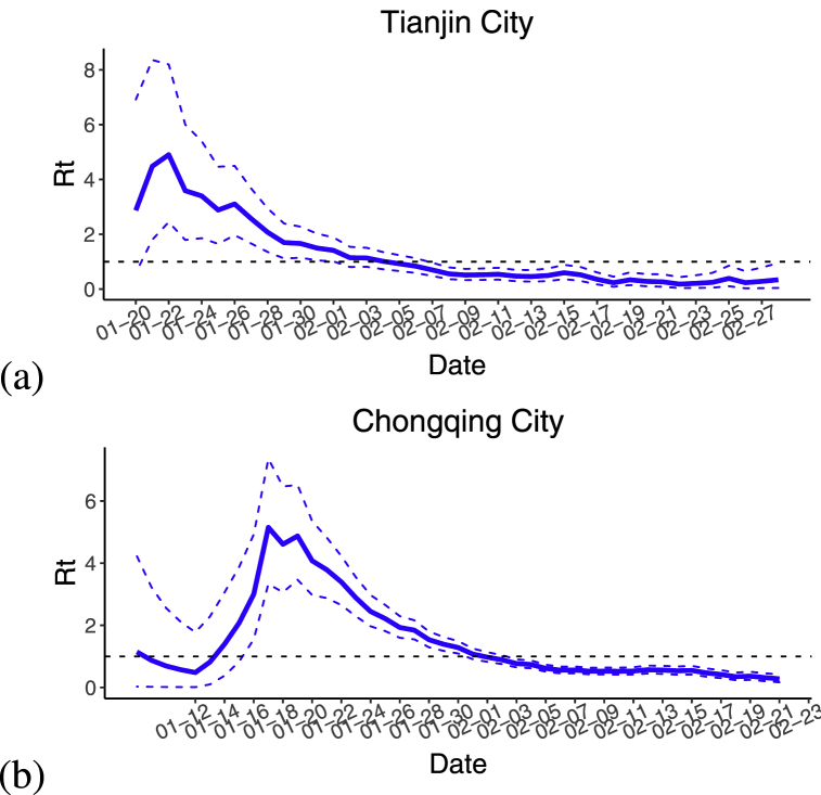
Based on the infected cases in Chongqing city and Tianjin City, the real-time regeneration number ${\mathcal{R}}_t$ of these two cities was calculated by using R language software and based on Bayesian framework, and the results were shown in Fig. 3. From Fig. 3, one can obtain that the real-time regeneration number in these two cities revealed a trend of rapidly rising, and then falling fast. The real-time regeneration number ${\mathcal{R}}_t$ of Tianjin is less than 1 after February 5, and the real-time regeneration number ${\mathcal{R}}_t$ of Chongqing is less than 1 after February 1, respectively. The real-time regeneration number ${\mathcal{R}}_t$ in Tianjin dropping below 1 was obviously later than that in Chongqing, which might be caused by the incident at the shopping mall in Baodi District of Tianjin. The shopping mall was the cluster of COVID-19 epidemic with the most confirmed cases, and had the most extensive influence in Tianjin. The initial decrease of ${\mathcal{R}}_t$ in Chongqing might due to the fact that most of the cases were imported in early January and did not spread widely in the local area. Later, during the Spring Festival travel rush, the population mobility was relatively large, which led to the rapid growth of ${\mathcal{R}}_t$.

Fig. 3.

Time series of real-time regeneration number ${\mathcal{R}}_t$, where the blue solid line represents the mean value of real-time regeneration number, and the blue dotted line represents the 95% confident interval of real-time regeneration number. (a) Tianjin City. (b) Chongqing City.

4.2. Parameter estimation and fitting results in Tianjin and Chongqing

By means of statistical analysis the life track of all laboratory-confirmed cases in Tianjin and Chongqing, we found that the last arrival time of imported case to Tianjin was January 31, 2020 (Also see Fig. 1 (a)), and there existed a sharp drop for symptom onset cases on February 05, 2020 in Chongqing. Hence, we divided the transmission of COVID-19 in Tianjin and Chongqing into two stages. The first stage data of COVID-19 epidemic in these two cities was used to give parameter estimation.

For the first stage, suppose that the initial value of the susceptible population S in Tianjin and Chongqing equal to 1.08163 × 10⁷ and 3.10179 × 10⁷, which is Year-end population of 2018 (China population & employ, 2019), and while all others (including L, E, I, A, Q, R, S_q) are 0. Human population birth and death rates were assumed $\mu =\frac{1}{365\ast 70}\approx 0.00004$. By counting the cumulative tracking quarantine cases of Tianjin and Chongqing on March 10, 2020, it was found that the quarantined people in these two cities were 2472 and 23677, respectively. Hence, we estimated the contact tracing isolation individuals per confirmed case b were about 2472/136 ≈ 18 and 23677/576 ≈ 41, respectively. For parameter γ, which depends on the actual situation of infected cases, and it also does not influence the model simulation. Therefore, we assume γ = 1/14.

Li et al. (2020a) obtained that the mean incubation period is 5.2 days (95% CI, 4.1–7.0 days) from a separate study of early COVID-19 cases. And He et al. (2020) inferred that infectiousness started from 2.3 days (95% CI, 0.8C3.0 days) before symptom onset. So we could obtain that the latent period and pre-symptomatic infectious period were 2.9 days and 2.3 days, respectively. Hence, one could obtain the values of d and δ were 1/2.9 and 1/2.3, respectively. Wang and Teunis (2020) collected the detailed data for 112 confirmed cases between 21 January 2020 and 12 February 2020 in Tianjin, and estimated the average serial interval was 4.8 days. It was easy to obtain the symptomatic infectious period was about 2.5 days and the value of c was 1/2.5 in Tianjin. Based on 77 transmission pairs obtained from publicly available sources within and outside mainland China, the serial interval was estimated to have a median of 5.2 days (95% CI, 4.1–6.4 days) based on a fitted gamma distribution (He et al., 2020). We assumed that the symptomatic infectious period was about 3 days and the value of c in Chongqing was 1/3. By means of statistical analysis of all laboratory-confirmed cases in Tianjin and Chongqing, we obtain the period between symptom onset and laboratory confirmation of the first stage are about 6 days and 9 days. So the period between symptomatic un-infectious and laboratory confirmation were 3.5 days and 6 days in Tianjin and Chongqing, respectively. And the value of m in these two cities were 1/3.5 and 1/6, respectively.

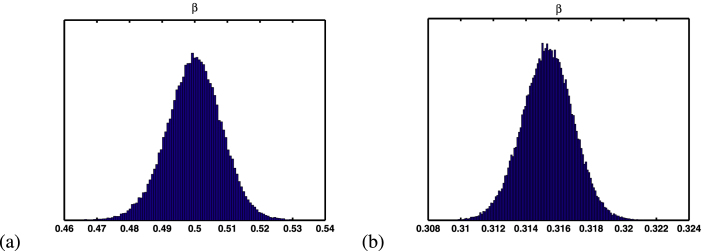
In previous paper (Li et al., 2020b), Li et al. assumed that the proportion between β₁ and β is 1/14, we also gave the same assumption. Hence, we only need to estimate the transmission rate β. In order to estimate the values of parameter β, we use extensive Markov-chain Monte-Carlo (MCMC) simulations based on the adaptive combination Delayed rejection and Adaptive Metropolis (DRAM) algorithm (Gamerman & Lopes, 2006; Haario et al., 2006) for system (2.1). Using 100000 sample realizations, we can acquire the parameter values for β with 1D parameter MCMC chain in Fig. 4. Then we further get the mean value, the standard deviation, MCMC error and Geweke for these parameters, which are shown in Table 1. From Fig. 4 and the value of Geweke, it is easy to see that the Markov-chain of parameters β of these two cities are convergent.

Fig. 4.

Simulation results for parameters β of MCMC chain with 100000 sample realizations. (a) Tianjin City. (b) Chongqing City. The Geweke convergence diagnostic method was employed to assess convergence of chains (Geweke et al., 1992), and the Geweke values of these two parameters are shown in Table 1.

Table 1.

Parameter estimation for β with the method of MCMC of Tianjin and Chongqing.

	Notation	Mean Value	Standard Deviation	Geweke
Tianjin	β	0.4998	0.0085	0.9992
Chongqing	β	0.3153	0.0016	0.9998

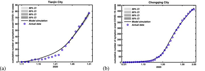
The time evolution of both infection cases and comparison with the symptom onset of COVID-19 cases in Tianjin and Chongqing were shown in Fig. 5, which also shows the 95% percent interval for all 100000 passing simulation trajectories and the median of these 100000 simulation outputs. It is clear that the theoretical prediction is nearly full agreement with real data, which also well validates the accuracy of proposed model.

Fig. 5.

Fitting results of cumulative number of symptom onset COVID-19 cases with its actual reported number with the method of MCMC. (a) Tianjin City. (b) Chongqing City.

For the second stage, the surveillance for new cases, and the tracing and management of contacts have been strictly performed, and people are suggested to stay at home as much as possible. Hence, we assume that the parameter β₁ is 0. By using the least square method, we can obtain the value of β in Tianjin and Chongqing are 0.0478 and 0.0679, respectively.

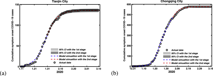
With the uncertainty for estimated parameters values, Monte Carlo simulation runs are then conducted to assess the performance of the model by using the available model parameters in Table 1. Fig. 6 unveils the prospect of the epidemic with cumulative of symptom onset COVID-19 cases in Tianjin and Chongqing City, shows the 95% percent interval for all 100000 passing simulation trajectories and the median of these 100000 simulation outputs.

Fig. 6.

The simulation result of cumulative number of symptom onset COVID-19 cases. (a) Tianjin City. (b) Chongqing City.

4.3. Local sensitivity analysis of ${\mathcal{R}}_0$

In this section, the normalized forward sensitivity indices (S.I.) of different quantities to the parameters of system (3.1) were computed and analyzed. The sensitivity indices of different quantities to any parameter p is given in (Kong et al., 2014) as

$$S.I.=\frac{\partial x^{\ast }}{\partial p}\frac{p}{x^{\ast }},$$

where x∗ is the quantity being considered. Sensitivity indices can be positive or negative which indicates the nature of the relationship, and it is the magnitude that ranks the strength of the relationship as compared to the other parameters. Here, $\frac{\partial x^{\ast }}{\partial p}$ could also be estimated by using the central difference approximation:

$$\frac{\partial x^{\ast }}{\partial p}=\frac{x^{\ast }(p+\mathrm{\Delta }p)-x^{\ast }(p-\mathrm{\Delta }p)}{2\mathrm{\Delta }p}+O(\mathrm{\Delta }{p}^2)$$

We choose Δp = 1% of p. Plugging all these in (8) we get

$$S.I.=\frac{x^{\ast }(1.01p)-x^{\ast }(0.99p)}{0.02x^{\ast }}.$$

We can look at the sensitivity of basic reproduction number ${\mathcal{R}}_0$ with respect to the parameters in Tianjin and Chongqing City (There exists the same level sensitivity of ${\mathcal{R}}_0$ with parameters in these two cities), which were shown in Table 2. The basic reproduction number ${\mathcal{R}}_0$ is most sensitive to the transmission rate β with a positive relationship and clinical outcome rate δ with a negative relationship. Therefore, reducing β or increasing δ will reduce the spread of disease when the focus of eradicating the disease is based on the reproduction number only. There is a weak relationship with the transmission rate β₁, birth rate μ, latent period rate d and transfer rate m for the basic reproduction number ${\mathcal{R}}_0$. Hence, these four parameters could not be chosen to be used as control parameters.

Table 2.

The sensitivity indices of ${\mathcal{R}}_0$.

Parameter	Chongqing	Tianjin	Description
β	0.9148	0.9280	Transmission rate from exposed to susceptible
β1	0.0852	0.0720	Transmission rate from infected to susceptible
d	1.16 × 10−4	1.16 × 10−4	Latent period rate
δ	−0.9148	−0.9280	Clinical outcome rate
μ	−2.18 × 10−4	−2.15 × 10−4	Human birth/death rate
c	−0.0852	−0.0720	Transfer rate from infectious to un-infectious

4.4. Simulation results with different lock-down strategy dates

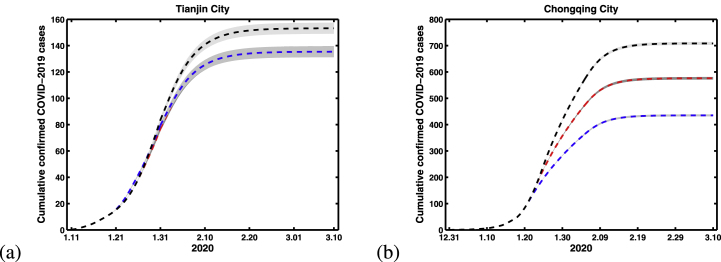
In China, the outbreak of COVID-19 was firstly reported in Wuhan city, then the confirmed cases from Wuhan started to appear in other Chinese provinces until 13 January 2020. The Chinese authorities introduced the implementation of the city lock-down strategy in Wuhan to shut down the movement on 23 January 2020. And the time of lock-down strategy in Wuhan affects the number of imported cases in other provinces. In this section, we want to explore that the impact of different Wuhan city lock-down dates for the cumulative confirmed COVID-19 cases in Tianjin and Chongqing. Fig. 7 show the simulation results with three different Wuhan city lock-down dates in Tianjin and Chongqing. In Tianjin, the dates of Wuhan city lock-down were not crucial in producing the outbreak pattern, because it’s mostly locally transmitted cases. The main reason is that there is a huge incident at the shopping mall in Baodi District on January 20. But in Chongqing, the dates of Wuhan city lock-down were crucial in producing the outbreak pattern, and it is obtained that the earlier with city lock-down, the fewer cases, and the later with city lock-down, the more cases. If the city lock-down date ahead two days, the final scale of cases will decrease about 150. And if the city lock-down date delay for two days, the mean final scale of cases will increase about 130.

Fig. 7.

Simulation results for cumulative number of confirmed COVID-19 cases with different lock-down strategy dates in Wuhan city. (a) Tianjin City. (b) Chongqing City. Where black, red and blue lines indicating the lock-down dates are 25 January, 23 January and 21 January, respectively.

4.5. Simulation results with different contact tracing isolation days

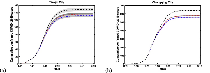
In China, some non-pharmaceutical interventions include strict controls on travel, extensive monitoring of suspected cases, and the contact tracing individuals with home quarantine for at least 14 days. The surveillance for new cases, and the tracing and management of contacts have been strictly performed (Li et al., 2020b). In this section, we will explore that the impact of different contact tracing isolation times for the cumulative confirmed COVID-19 cases in Tianjin and Chongqing. Fig. 8 show the simulation results with three different contact tracing isolation times in Tianjin and Chongqing. It is obtained that the more contact tracing isolation days on confirmed cases, the fewer cases, and the less days, the more cases. But it is not sensitive for the more contact tracing isolation days on confirmed cases, the fewer cases when tracing isolation days reaches a certain value (See the red and blue lines of Fig. 8). Hence, the quarantine time of contact tracing for 14 days is the most comfortable time.

Fig. 8.

Simulation results for cumulative number of confirmed COVID-19 cases with different contact tracing isolation times. (a) Tianjin City. (b) Chongqing City. Where black, red and blue lines indicating the contact tracing isolation times are 7, 14 and 21 days, respectively.

5. Discussion and conclusions

The spread of COVID-19 in 2020 has brought substantial economic losses to mainland China. Government has been seeking various prevention and control measures to drastically reduce within-population contact rates and transmission to prevent infection and further transmission of COVID-19. All transport was prohibited in and out of Wuhan city from 23 January 2020, and quarantine of both suspected individuals and subjects who have had close contacts with suspected cases. By the end of February 2020, the COVID-19 epidemic of China has been basically controlled in all provinces and cities except Hubei province.

In this study, to investigate the underlying dynamics of COVID-19 transmission and the effectiveness of early prevention and control measures with the tracing isolation of close contacts of newly confirmed cases in some provinces (such as Tianjin and Chongqing city) except Hubei Provinces, make predictions and perform assessment and risk analysis for COVID-19 outbreaks, we developed a differential equation model with tracing isolation strategy for close contacts of newly confirmed cases and discrete time imported cases. Firstly, we gave some dynamic analysis of the proposed model including the basic reproduction number, the stability of disease-free equilibrium, and the existence and uniqueness of positive equilibrium. Then, the real-time regeneration number ${\mathcal{R}}_t$ of these two cities were shown in Fig. 3. The real-time reproduction number in these two cities revealed a trend of rapidly rising, and then falling fast.

Finally, some numerical simulations with system (2.1) were given by using the detailed infectious cases of Tianjin and Chongqing. Markov-chain Monte-Carlo (MCMC) simulations based on the adaptive combination Delayed rejection and Adaptive Metropolis (DRAM) algorithm was used to give parameter estimation with system (2.1) in Tianjin and Chongqing. In our simulation, the disease disappeared in late February in these two cities and it was the same with the actual situation. Sensitivity analysis demonstrate that the dates of Wuhan city lock-down were not crucial in producing the outbreak pattern in Tianjin, because it’s mostly locally transmitted cases. But in Chongqing, the dates of Wuhan city lock-down were crucial in producing the outbreak pattern, and it is obtained that the earlier with city lock-down, the fewer cases, and the later with city lock-down, the more cases. By analyzing the influence with different close contact tracing isolation days for the cumulative confirmed COVID-19 cases. Our study found that the tracing isolation of close contacts of newly confirmed cases could effectively control the spread of the disease. One can obtain that the more contact tracing isolation days on confirmed cases, the fewer cases. But it is not sensitive for the more contact tracing isolation days on confirmed cases, the fewer cases.

In this work, we focused on the transmission of COVID-19 with the tracing isolation of close contacts of newly confirmed cases in Tianjin and Chongqing city, China. If the data is relevant and sufficient for other provinces, our model can also be applied to these related provinces spread of COVID-19 in mainland China.

Declaration of competing interest

The authors declare that they have no competing interests.

Handling editor: Dr HE DAIHAI HE

References

- Castillo-Chavez C., Song B.J. Dynamical models of tuberculosis and their applications. Mathematical Biosciences and Engineering. 2004;2(1):361–404. doi: 10.3934/mbe.2004.1.361. [DOI] [PubMed] [Google Scholar]
- Chen T.M., Rui J., Wang Q.P., Zhao Z.Y., Cui J.A., Yin L. A mathematical model for simulating the phase-based transmissibility of a novel coronavirus. Infectious Diseases of Poverty. 2020;1(9):1–8. doi: 10.1186/s40249-020-00640-3. [DOI] [PMC free article] [PubMed] [Google Scholar]
- China population & employment statistics yearbook. China Statistics Press; Beijing: 2019. [Google Scholar]
- Chinazzi M., Davis J.T., Ajelli M., Gioannini C., Litvinova M., Merler S.…Vespignani A. The effect of travel restrictions on the spread of the 2019 novel coronavirus (2019-nCoV) outbreak. Science. 2020 doi: 10.1126/science.aba9757. [DOI] [PMC free article] [PubMed] [Google Scholar]
- Cori A., Ferguson N.M., Fraser C., Cauchemez S. A new framework and software to estimate time-varying reproduction numbers during epidemics. American Journal of Epidemiology. 2013;178(9):1505–1512. doi: 10.1093/aje/kwt133. [DOI] [PMC free article] [PubMed] [Google Scholar]
- Diekmann O., Heesterbeek J.A.P., Metz J.A. On the definition and the computation of the basic reproduction ratio R0 in models for infectious diseases in heterogeneous populations. Journal of Mathematical Biology. 1990;28:365–382. doi: 10.1007/BF00178324. [DOI] [PubMed] [Google Scholar]
- Diekmann O., Heesterbeek J.A.P., Roberts M. The construction of next-generation matrices for compartmental epidemic models. Journal of the Royal Society Interface. 2009;7:873–885. doi: 10.1098/rsif.2009.0386. [DOI] [PMC free article] [PubMed] [Google Scholar]
- van den Driessche P., Watmough J. Reproduction numbers and sub-threshold endemic equilibria for compartmental models of disease transmission. Mathematical Biosciences. 2002;180:29–48. doi: 10.1016/s0025-5564(02)00108-6. [DOI] [PubMed] [Google Scholar]
- Du Z., Wang L., Cauchemez S., Xu X., Wang X., Cowling B.J., Meyers L.A. Risk for transportation of 2019 novel coronavirus disease from Wuhan to other cities in China. Emerging Infectious Diseases. 2020;26(5):1049–1052. doi: 10.3201/eid2605.200146. [DOI] [PMC free article] [PubMed] [Google Scholar]
- Gamerman D., Lopes H.F. 2nd ed. Taylor and Francis Group; London New York: 2006. Markov chain monto carlo: Stochastic simulation for bayesian inference. [Google Scholar]
- Geweke J. Evaluating the accuracy of sampling-based approaches to the calculation of posterior moments. In: Bernardo J.M., Berger J., Dawid A.P., Smith A.F.M., editors. Bayesian statistics 4. Oxford University Press; Oxford: 1992. pp. 169–193. [Google Scholar]
- Haario H., Laine M., Mira A., Saksman E. Dram: Efficient adaptive mcmc. Statistics and Computing. 2006;16:339–354. [Google Scholar]
- He X., Lau E.H., Wu P., Deng X.L., Wang J., Hao X.X.…Leung G.M. Temporal dynamics in viral shedding and transmissibility of COVID-19. Nature Medicine. 2020;26:672–C675. doi: 10.1038/s41591-020-0869-5. [DOI] [PubMed] [Google Scholar]
- Kong J.D., Davis W., Li X., Wang H. Stability and sensitivity analysis of the iSIR model for indirectly transmitted infectious diseases with immunological threshold. SIAM Journal on Applied Mathematics. 2014;5(74):1418–1441. [Google Scholar]
- LaSalle J.P. Regional conference series in applied mathematics. SIAM Philadelphia; 1976. The stability of dynamical systems. [Google Scholar]
- Li Q., Guan X., Wu P., Wang X.Y., Zhou L., Tong Y.Q., Ren R.Q., Leung K.S.M., Lau E.H.Y., Wong J.Y., Xing X.S., Xiang N.J., Wu Y., Li C., Chen Q., Li D., Liu T., Zhao J., Liu M., Feng Z.J. Early transmission dynamics in Wuhan, China, of novel coronavirus-infected pneumonia. New England Journal of Medicine. 2020;382(13):1199–1207. doi: 10.1056/NEJMoa2001316. [DOI] [PMC free article] [PubMed] [Google Scholar]
- Lin Q.Y., Zhao S., Gao D.Z., Lou Y.J., Yang S., Musa S.S., Wang M.H., Cai Y.L., Wang W.M., Yang L., He D.H. A conceptual model for the coronavirus disease 2019 (COVID-19) outbreak in Wuhan, China with individual reaction and governmental action. International Journal of Infectious Diseases. 2020;93:211–216. doi: 10.1016/j.ijid.2020.02.058. [DOI] [PMC free article] [PubMed] [Google Scholar]
- Li M.T., Sun G.Q., Zhang J., Zhao Y., Pei X., Wang Y., Zhang W.Y., Zhang Z.K., Jin Z. Analysis of COVID-19 transmission in Shanxi Province with discrete time imported cases. Mathematical Biosciences and Engineering. 2020;4(17):3710–3720. doi: 10.3934/mbe.2020208. [DOI] [PubMed] [Google Scholar]
- Smith H.L., Waltman P. Cambridge University Press; 1995. The theory of the chemostat. [Google Scholar]
- Sun G.Q., Wang S.F., Li M.T., Li L., Zhang J., Zhang W., Jin Z., Feng G.L. Transmission dynamics of COVID-19 in Wuhan, China: Effects of lockdown and medical resources. Nonlinear Dynamics. 2020;101(3):1981–1993. doi: 10.1007/s11071-020-05770-9. [DOI] [PMC free article] [PubMed] [Google Scholar]
- Tang B., Bragazzi N.L., Li Q., Tang S.Y., Xiao Y.N., Wu J.H. An updated estimation of the risk of transmission of the novel coronavirus (2019-nCov) Infectious Disease Modelling. 2020;5:248–255. doi: 10.1016/j.idm.2020.02.001. [DOI] [PMC free article] [PubMed] [Google Scholar]
- Tang S.Y., Tang B., Bragazzi N.L., Xia F., Li T.J., He S., Ren P.Y., Wang X., Xiang C.C., Peng Z.H., Wu J.H., Xiao Y.N. Analysis of COVID-19 epidemic traced data and stochastic discrete transmission dynamic model (in Chinese) Scientia Sinica Mathematica. 2020;50:1–16. [Google Scholar]
- Tang B., Wang X., Li Q., Bragazzi N.L., Tang S.Y., Xiao Y.N., Wu J.H. Estimation of the transmission risk of the 2019-nCoV and its implication for public health interventions. Journal of Clinical Medicine. 2020;9(2):462. doi: 10.3390/jcm9020462. [DOI] [PMC free article] [PubMed] [Google Scholar]
- Wang Y., Teunis P. Strongly heterogeneous transmission of COVID C19 in mainland China. Frontiers of Medicine. 2020;7:329. doi: 10.3389/fmed.2020.00329. [DOI] [PMC free article] [PubMed] [Google Scholar]
- White L.F., Pagano M. A likelihood-based method for real-time estimation of the serial interval and reproductive number of an epidemic. Statistics in Medicine. 2008;16(27):2999–3016. doi: 10.1002/sim.3136. [DOI] [PMC free article] [PubMed] [Google Scholar]
- Wu J.T., Leung K., Leung G.M. Nowcasting and forecasting the potential domestic and international spread of the 2019-nCoV outbreak originating in Wuhan, China: A modelling study. The Lancet. 2020;395(10225):689–697. doi: 10.1016/S0140-6736(20)30260-9. [DOI] [PMC free article] [PubMed] [Google Scholar]
- Yang Z.F., Zeng Z.Q., Wang K., Wong S.S., Liang W.H., Zanin M., Liu P., Cao X.D., Gao Z.Q., Mai Z.T., Liang J.Q., Liu X.Q., Li S.Y., Li Y.M., Ye F., Guan W.J., Yang Y.F., Li F., Luo S.M., He J.X. Modified SEIR and AI prediction of the epidemics trend of COVID-19 in China under public health interventions. Journal of Thoracic Disease. 2020;12(3):165–174. doi: 10.21037/jtd.2020.02.64. [DOI] [PMC free article] [PubMed] [Google Scholar]