Estimation of undetected symptomatic and asymptomatic cases of COVID‐19 infection and prediction of its spread in the USA

Abstract

The reported COVID‐19 cases in the United States of America have crossed over 10 million and a large number of infected cases are undetected whose estimation can be done if country‐wide antibody testing is performed. In this study, we estimate this undetected fraction of the population by a modeling and simulation approach. We employ an epidemic model SIPHERD in which three categories of infection carriers, symptomatic, purely asymptomatic, and exposed are considered with different transmission rates that are taken dependent on the social distancing conditions, and the detection rate of the infected carriers is taken dependent on the tests done per day. The model is first validated for Germany and South Korea and then applied for prediction of the total number of confirmed, active and dead, and daily new positive cases in the United States. Our study predicts the possible outcomes of the infection if social distancing conditions are relaxed or kept stringent. We estimate that around 30.1 million people are already infected, and in the absence of any vaccine, 66.2 million (range: 64.3–68.0) people, or 20% (range: 19.4–20.5) of the population will be infected by mid‐February 21 if social distancing conditions are not made stringent. We find the infection‐to‐fatality ratio to be 0.65% (range: 0.63–0.67).

1. INTRODUCTION

The outbreak of pandemic Coronavirus disease 2019 (COVID‐19) has led to more than 50 million total reported infections and 1.2 million deaths worldwide (https://www.worldometers.info/coronavirus) and serious efforts are needed for its containment. The Coronavirus SARS‐CoV‐2 has affected not just public health but had a drastic impact on the economy of the world as well, due to the lockdown situations in many countries, including the United States of America. In the United States of America, the first positive case of COVID‐19 was reported on January 20, 2020, in a man who returned from Wuhan, China, where the outbreak was first identified, and the first death took place in the first week of February. ¹ A major control measure was announced on March 16, restricting the gathering of more than ten people. However, the COVID‐19 spread to almost 50 states throughout the country by March‐end (https://www.worldometers.info/coronavirus). ² Now, the United States of America has become the most affected country in terms of confirmed, active, and death cases in the world (https://www.worldometers.info/coronavirus).

Pandemics have hit humanity many times in the past also, and mathematical models are already available for infectious diseases. ³ , ⁴ , ⁵ , ⁶ Mathematical modeling of the epidemic has an unavoidable role in helping the healthcare sector by predicting the hospital requirements in advance and for setting up the critical care systems for the patients. ⁷ , ⁸ To devise the lockdown strategy, it is imperative that the prediction of the disease spread is available to the policymakers. COVID‐19 is different from the previously known SARS (severe acute respiratory syndrome) infection, with features such as the existence of purely asymptomatic cases ⁹ and the spread of the infection from those as well as from the exposed ones in the incubation period. ¹⁰ Our proposed mathematical model incorporates the above facts for the COVID‐19 epidemic.

Many epidemiological models exist in the literature, and the basic SIR model ¹¹ is the widely used one, which needs to be modified to incorporate the peculiar features involved in Coronavirus spread and control. An approximate mathematical model of the COVID‐19 was initially reported in the literature ¹² based on the Between‐Countries Disease Spread and the study shows that the United States of America has the highest daily probability of receiving one infected person from other infected countries. An improved mathematical model for the spread of COVID‐19 is proposed in Reference [13], by taking into account the infected and undetected cases. But this study and forecast are particularly based only on China. An extended susceptible–infected–recovered (SIR) model is proposed in Reference [14], in which the entire people in the country are divided into eight compartments. Though it is an improved version of the SIR model, the study and simulation results are done only for Italy, and the model does not take into account purely asymptomatic cases and the role of tests done per day (TPD). Another compartmental epidemic model SEIR (susceptible–exposed–infectious–recovered) ¹⁵ forecast for few countries and the impact of the quarantine on the COVID‐19 is investigated. A stochastic epidemic model is presented in Reference [16], where the effect of clinical progression and transmission network structure on the outcome of social distancing is investigated. An adaptive and improved version of the SIR model is illustrated in Reference [17]. In this method, the time dependency of parameters used for the analysis makes it more robust than the conventional SIR method. Curve fitting‐based methods have been also employed for the forecast of COVID‐19 in References [18, 19, 20]. Although these methods can track the available data correctly, they are not developed based on the physical insights that affect the rate of spreading of the disease, and also it is extremely sensitive to the initial conditions. In Reference [21], Murray and his collaborators predicted the number of hospital beds that will be needed, critical healthcare requirements like intensive care units and ventilators based on the data of present COVID‐19 patients, and the total number of deaths in the United States and the European Economic Area.

In this paper, we formulate a mathematical model, named SIPHERD for the COVID‐19 epidemic and apply it for forecasting the number of total active and confirmed cases, daily new positive and death cases in the United States of America, according to the conditions of the social distancing and the number of tests performed per day. The model has been applied for the prediction of COVID‐19 spread in India. ²²

2. METHODS

2.1. Mathematical model SIPHERD

We model the dynamics of the COVID‐19 disease spread by dividing the population into different categories, as listed below.

• S—Fraction of the total population that is healthy and has never caught the infection

• E—Fraction of the total population that is exposed to infection, transmit the infection and turn into either symptomatic or purely asymptomatic, and not detected

• I—Fraction of the total population infected by the virus that shows symptoms and undetected

• P—Fraction of the total population infected by the virus that doesn't show symptoms even after the incubation period and undetected. These are the purely asymptomatic cases

• H—Fraction of the total population that are found positive in the test and either hospitalized or quarantined

• R—Fraction of the total population that has recovered from the infection

• D—Fraction of the total population that is deceased due to the infection.

The SIPHERD model equations are a set of coupled ordinary differential Equation (1) for the defined entities (S, I, P, H, E, R, D). As seen in Figure 1, the rates of transfer from one category to another are the model parameters, and a set of differential equations for the entity in each category is formed. We write the model equations that are independent of the population of the country by considering the fraction of the people in each category. The various rates listed in Table 1 are the parameters of the problem which are not known, and only the possible range is available and the initial conditions E(0), P(0), and I(0) are also not exactly known. Some of the parameters such as rates of infection (α, β, γ) change with time in steps, depending on the lockdown and social distancing conditions, and the probability rate of detection (ν) changes with time depending on TPD. The model equations are written as

$$\begin{array}{ccc}\frac{\mathit{dS}}{\mathit{dt}}& =& -S\left(\alpha E+\beta I+\gamma P+\delta H\right),\\ \frac{\mathit{dE}}{\mathit{dt}}& =& S\left(\alpha E+\beta I+\gamma P+\delta H\right)-\left(\mu +{\xi }_I+{\xi }_P\right)E,\\ \frac{\mathit{dH}}{\mathit{dt}}& =& \mu \left(E+P\right)+\nu I-\sigma H\left(t-t_R\right)-\tau H\left(t-t_D\right),\\ \frac{\mathit{dI}}{\mathit{dt}}& =& {\xi }_{I}E-\left(\nu +\omega \right)I,\\ \frac{\mathit{dP}}{\mathit{dt}}& =& {\xi }_{P}E-\left(\mu +\eta \right)P,\\ \frac{\mathit{dR}}{\mathit{dt}}& =& \omega I+\eta P+\sigma H\left(t-t_R\right),\\ \frac{\mathit{dD}}{\mathit{dt}}& =& \tau H\left(t-t_D\right).\end{array}$$ (1)

where, tR and tD are the delay associated with the recovery and death, respectively, with respect to active cases H. We have taken into account this delay because the active cases are reported after the testing and admission to healthcare or quarantine center, and the number of recovery and death of the admitted will not immediately follow the active or H category number and there will be a certain average time delay between a COVID‐19 positive case detection and the recovery or the death. We take the value of tR and tD to be 12 and 14 days respectively. All fractions add up to unity that can also be seen from summing the above equations,

$$\frac{d}{\mathit{dt}}(S+I+P+H+E+R+D)=0.$$ (2)

Figure 1.

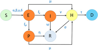
Schematic of the SIPHERD Model: α, β, γ, δ are rates of transmission of infection; ξ _I, ξ _P are rates of transfer from being exposed to symptomatic and asymptomatic; ω, η, σ are recovery rates; μ, ν are detection rates, and τ is the mortality rate

Table 1.

Parameters of the SIPHERD model

Parameter	Description
α	Rate of transmission of infection from E to S
β	Rate of transmission of infection from I
γ	Rate of transmission of infection from P to S
δ	Rate of transmission of infection from H to S
ξ I,p	Rate of conversion from the E to I, P
σ	Rate of recovery of H
ω	Rate of home recovery of I
η	Rate of home recovery of P
µ	Probability of E and P being detected
ν	Probability of I being detected
τ	Mortality Rate

The probability of getting the infection is assumed uniform among the susceptible people, although the disease spreads are localized in hot‐spots. Therefore, even though the disease has spread very differently in different US states, the model considers the “average effect” for the estimation of the infected and death cases.

The basic reproduction number (R ₀) can be written by observing the inflow and outflow rates for each infectious category (E, I, P, H) shown in Figure 1. The contribution of each of these categories for the reproduction number can be written as the ratio of the sum of inflow rates and the sum of outflow rates multiplied by the rate of transmission of infection of that category,

$$R_0\mathrm{\Omega }=\alpha +\frac{{\xi }_I\beta }{\nu +\omega }+\frac{{\xi }_P\gamma }{\mu +\eta }+\frac{\delta }{\sigma +\tau }\left(\mu +\frac{{\xi }_I\nu }{\nu +\omega }+\frac{{\xi }_P\mu }{\mu +\eta }\right),$$ (3)

where $\mathrm{\Omega }=\mu +{\xi }_I+{\xi }_P$. As the existence of purely asymptomatic cases are a distinct feature of COVID‐19, and it is crucial to identify the proportion of such cases among the total infected to build a realistic model. The Diamond Princess Cruise study is the key to identify the proportion of Asymptomatic cases as all the susceptible people onboard were tested. The asymptomatic proportion of the infected persons on board the Diamond Princess Cruise is estimated in Reference [9]. Among the 634 tested positive onboard, 328 were found asymptomatic, that is, more than 50% of the confirmed cases were not showing any specific symptoms of COVID‐19. The ratio of purely asymptomatic (P) to total asymptomatic (E+P) cases is reported to be 0.35, and the ratio of purely asymptomatic to the total infected (E+P+I) is 0.179. ⁹

The above‐observed ratios can be written in terms of the entities on the Cruise (with a bar) as all the people onboard were tested,

$$\frac{\stackrel{\leftharpoonup }{P}}{\stackrel{\leftharpoonup }{P}+\stackrel{\leftharpoonup }{E}}=0.35,\frac{\stackrel{\leftharpoonup }{P}}{\stackrel{\leftharpoonup }{P}+\stackrel{\leftharpoonup }{E}+\stackrel{\leftharpoonup }{I}}=0.179.$$ (4)

This implies that $\stackrel{\leftharpoonup }{P}$/$\stackrel{\leftharpoonup }{I}$ = 0.36. These reported numbers are used to fix the proportion between ξ _P and ξ _I as 0.36 and the proportion of initial conditions E(0), I(0), and P(0) as well. In other words, out of 136 exposed cases, after the incubation, 36 will turn to be purely asymptomatic, and 100 will have symptoms.

The detection of the asymptomatic and symptomatic cases can be taken dependent on the number of tests done per day (T _PD). For the symptomatic cases, the detection is more probable as the infected person can approach for the tests and more likely to be tested. The detection of symptomatic is taken in two parts, a constant (ν ₀) and another part proportional to the TPD. This can be written in terms of parameters as

$$\nu ={\nu }_0+{\nu }_1{T}_{\mathrm{PD}},$$ (5)

$$\mu ={\mu }_0{T}_{\mathrm{PD}},$$ (6)

where, µ ₀, ν ₀, and ν ₁ are positive constants. The total confirmed cases are the addition of the active cases, extinct cases, and a part of the recovered that were detected. This can be written as

$$C\left(t\right)=H\left(t\right)+D\left(t\right)+{\int }^t\sigma H(\tau \text{'})d\tau \text{'}.$$ (7)

Asymptomatic carriers of Coronavirus‐nCoV2 do transmit the disease. Also, the infection can be transmitted from the person who is not showing illness during the incubation period. ¹⁰ This is included in the model by considering E category people and their transmission rate α. Hospitalized and quarantined cases can also transmit the disease, and this low rate is taken as parameter δ. We model the transmission rate of infection change with time in steps, depending on the conditions of the lockdown. The transfer rate from E to I (ξ _I) is the inverse of the incubation period, whose mean is reported 5.2 days. ²³  The recovery time of symptomatic cases is taken as 14 days. The rate of transmission of infection from the asymptomatic carrier (α, γ) for a country is typically taken higher than the symptomatic ones (β) as the asymptomatic carrier may not be aware of his/her infection, and Susceptible may not be keeping distance as no symptoms are seen. The mortality rate (τ) is taken differently for different countries as it depends on the immunity and how effectively the critical patients are taken care of by the hospitals.

2.2. Optimization of the parameters

Some of the parameters namely, ω, η, ξ _P, ξ _I have a fixed value as those represent the characteristics of the disease itself. The remaining parameters are to be obtained that generate the evolution of the dynamical system close to the actual data. Manual tuning of the parameters for the best fit is quite a tedious task. For this purpose, we write a cost function in terms of the standard deviation from the actual data and model data for the confirmed and the active cases as the following:

$${\mathrm{COST}}_1\left({\rho }_j\right)=\sum _i{(C_i^{\mathrm{data}}-C_i^{\mathrm{mod}})}^2+{(H_i^{\mathrm{data}}-H_i^{\mathrm{mod}})}^2,$$ (8)

where ρ _j are the different parameters that are to be obtained. For estimation of the undetected infected cases for the United States of America, we write another cost for the first 40 days from March 1, 2020,

$${\mathrm{COST}}_2\left({\rho }_j\right)={\sum }_i^{40}{\left(E_i{\xi }_I{P}_{SI}-{\mathrm{DNC}}_{i+t_S}^{\mathrm{data}}\right)}^2,$$ (9)

where P _SI is the probability of the daily new symptomatic cases develop severe symptoms after a time delay of t _S days and were reported as daily new cases (DNC). The net cost function is the sum of COST₁ and COST₂.

A MATLAB function “fmincon” is used to find the minimum of a problem depending on a set of parameters that can have upper and lower bounds. fmincon returns the set of parameters within the given range, which minimizes the COST function defined above. As there could be multiple sets of parameters giving out “good fit” to the real data, other physical constraints on the parameter sets can be considered. One of them is a reasonable value of the reproduction number. Second, the rate of transmission of infection before lockdown has to be greater than after lockdown. The mortality rate (τ) is not optimized but rather calculated directly by the daily number of deaths data (DND) and the active data. The mortality rate for a particular day can be obtained as follows:

$$\tau \left(i\right)=\frac{\mathrm{DND}\left(i\right)}{H(i-t_D)}.$$ (10)

2.3. Numerical implementation and simulation

The set of coupled equations for the model for a given set of parameters and initial values is solved numerically by the dde23 solver routine of MATLAB for ordinary differential equations with a time lag in functions. The nontrivial part is the accurate determination of the parameters that will mimic the situation on the ground. The mathematical problem is to take into account the actual data sets of the total number of confirmed cases, active cases on a particular day, cumulative deaths, and TPD and find the set of parameters that will provide the best possible match between the data and model. The extraction of the parameters is automated so that the model can be run on data for various countries. The minimizer of the cost is found to obtain the optimized set of parameters that best fit with the data available to date. The model and the optimization scheme are implemented in MATLAB. The parameters determined by our model are listed in Table 2 for the countries we studied.

Table 2.

Parameters values for the countries studied

Parameters	Germany	South Korea	United States of America
Population (N)	8.30E7	5.10E7	3.31E8
T 0	Feb 21	Feb 15	Mar 1
TLD	29, 37	18	25, 36, 100, 140, 195, 210, 230
α (bf. LD)	0.35	0.45	0.38
α (af. LD)	0.23, 0.14	0.17	0.07, 0.08, 0.062, 0.077, 0.086, 0.095, 0.12
β (bf. LD)	0.19	0.16	0.25
β (af. LD)	0.18, 0.11	0.11	0.064, 0.053, 0.16, 0.08, 0.08, 0.11, 0.11
γ (bf. LD)	0.35	0.45	0.38
γ (af. LD)	0.23, 0.14	0.17	0.07, 0.08, 0.062, 0.077, 0.086, 0.095, 0.12
δ	9E−3	5.9E−3	6E−3
ξ I	0.2	0.2	0.2
ξP	0.072	0.072	0.072
µ 0	1.67E−6	2.05E−5	0
ν 0	0.05	0.07	0.027
ν 1	4.7E−6	9.7E−5	7.5E−8
ω	0.07	0.07	0.07
η	0.1	0.1	0.1
σ	0.065	0.034	0.017
tR	6	11	14
tD	6	1	12
Initially Infected	100	150	1000

Abbreviations: LD, lockdown; af., after; bf., before; TLD, number of days lockdown or change in social distancing conditions occurred after T0; T0, starting date for the simulation.

For the United States of America, the rate of transmission of infection is taken to change in eight steps. This is done by plotting the total number of cases on a log scale and seeing the changes in the slopes and correlating with the government's regulations on social activities. As seen in Figure S3b, we fit the actual mortality rate in steps. It can be seen that the mortality rate improved with time. The mortality rate is expected to improve further, as mild cases will also be reported with more tests available. The probability P _SI of symptomatic patients developing severe symptoms such as breathlessness, high fever, and so forth, has definitely approached the test and was tested in the initial phases. Data from cases reported from 49 states, the District of Columbia, and three US territories to CDC from February 12–March 16 shows that 20.7 reported cases were hospitalized (https://gis.cdc.gov/grasp/covidnet/COVID19_3.html). COVID‐NET regions show it to be 21.4% till April 4 (https://covid19.healthdata.org/united-states-ofamerica) ²⁴ and IHME data (March 5–April 4) shows that to be 20.3% (https://covid19.healthdata.org/united-states-ofamerica). ²⁰ The estimation of the total infected to hospitalized is reported to be 3.6% in another study for France. ²⁵ Therefore, we estimate the total 17% (3.6/0.21) of the total infected develop symptoms that are not mild and are tested and reported in the initial days. In China, this number of non‐mild cases is reported to be 19%. ²⁶ For the first 40 days, we put a COST for the above condition that every day, 20% (ξ _I) of the exposed develop symptoms, and 17% of them are reported as daily new cases with an average delay of 5 days. It can be seen from Figure S4d that this condition is indeed satisfied, as the model curve and real data overlap for the first few days. Later, the gap between the two curves widens as more tests were made available and mild cases also tested.

The projection for the total infected persons is strongly dependent on the value of P _SI, which we estimate to be 17% as discussed above. We simulate two more situations for the P _SI value 15% and 19% and plot the time dependence of the Susceptible and Extinct cases in Figure S4.

2.4. Data collection

We collected the data from the following publicly available data sources: The total number of cases, active cases, daily new cases, and total and daily new deaths is collected from the worldometer (https://www.worldometers.info/coronavirus). Test‐per‐day data is collected from https://ourworldindata.org/grapher/full-list-covid19-tests-per-day. Hospitalization data are collected from https://covid19.healthdata.org/united-tates-ofamerica,gis.cdc.gov/grasp/covidnet/COVID19_3.html, and Reference [27].

The day on which lockdown is imposed or social distancing conditions changed in a country is also taken into account as changes in the slopes of the data for confirmed cases are observed according to it.

3. RESULTS AND DISCUSSION

We apply the SIPHERD model to South Korea and Germany for testing the predictive capability of our model. We used the data only for the first 20 and 40 days, respectively, that is, till March 5 and March 31, 2020, and compared the future evolution generated by the model with the actual data, as shown in the gray region in Figure 2A for South Korea and in Figure 2B for Germany. Parameters extracted by the model from the actual data for the countries studied are listed in Table 2. These particular countries are chosen just for validation of our model and not for comparison with the United States of America.

Figure 2.

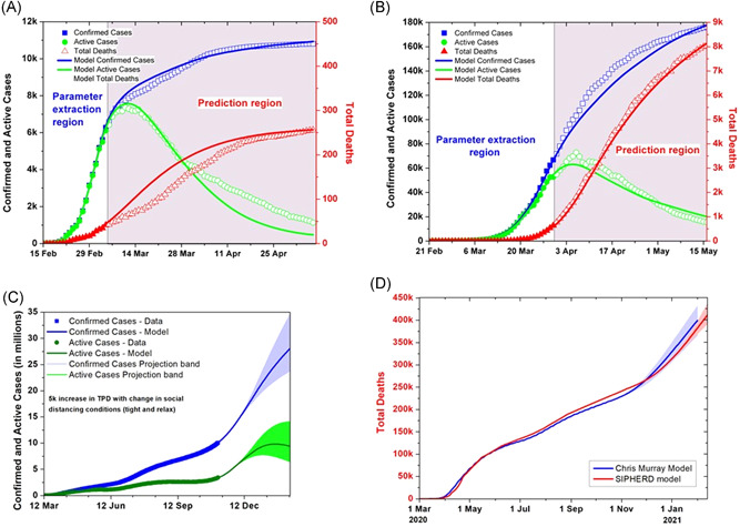
Model predictions for South Korea, Germany, and the United States of America (USA). (A) South Korea data are given to the simulator upto March 5, and thereafter, model comparison with the actual data for the confirmed, active cases and total deaths. (B) Model prediction using the German data upto March 31 and comparison with the actual data for the confirmed, active cases and total deaths. (C) Comparison of the model prediction for the USA if the social distancing and lockdown conditions kept same, made stringent, and relaxed after November 26, while the tests increased by 5000 daily for both scenarios. (D) SIPHERD Model compared with the “Cris Murray Mode” for the projection of the extinct cases

3.1. Effect of social distancing

The model, thus validated, is then applied to the existing data of the United States of America for the prediction of the next 350 days, that is, till February 13, 2021, as shown in Figure 2C. Three scenarios are considered for social distancing conditions. One possible scenario is that the conditions are kept the same, the second one is that they are relaxed after November 26, and the third is if they are made more stringent. TPD assumed to be increased by 5000 for all three scenarios. The transmission rate for the relaxed social distancing conditions is taken as 100%, 90% of the current value, and for the mean case 90%, 80% of the current value, and for the stringent conditions 80%, 70% of the current value, after 20 and 50 days from November 6, respectively. The mortality rate is calculated from the data and is improved in steps from an initial value of 2.8% on March 1 to 0.03% on November 6 as seen in Figure S3b.

The projection of the “Chris Murray” model is compared with the SIPHERD model for the total number of deaths in Figure 2D. The prediction range of the “Chris Murray” Model can be seen as large compared to the SIPHERD model.

Two scenarios are demonstrated in Figure 3D in which social distancing is made stringent for a month from November 26 such that the rate of transmission decreases to 60% to current value and then kept at 80% of the current value; whereas, in the other scenario it is kept at 80% after November 26. It can be seen that strict conditions on social distancing for a month can be an effective strategy. We also report on a couple of additional scenarios for prediction in the Supporting Information Material. If the social distancing is kept the same for the month after November 26, then how fast the disease will spread for 5000 increase in TPD is also plotted in Figure S5. If the conditions are made stricter only for 1 month and if it is relaxed after 1 month, the evolution can be seen in Figure S6. The reproduction number is seen to go beyond one in the month for the current relaxed conditions.

Figure 3.

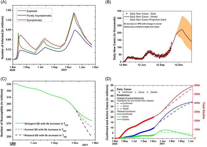
Undetected cases and effect of social distancing (SD). (A) The evolution of the undetected number of Infected in the exposed (E), symptomatic (I), and purely asymptomatic (P) category with SD conditions kept the same. (B) Model prediction for daily new cases for USA with the increase of 5000 tests per day with lockdown and SD conditions kept the same till November 26. (C) The evolution of the Susceptible when SD situations kept same and relaxed after November 26 with tests per day increase by 5000. (D) Prediction when SD situations relaxed and kept stringent for a month after November 26 to the extent that rate of transmission of infection changes by 10%

3.2. Estimation of the undetected cases

As only symptomatic cases were tested, the detection probability of asymptomatic (µ) is taken zero. There can be many parameter sets, including the probability rate of detection of symptomatic ν, that give a good match between the simulation results and the actual data. It is, therefore, not possible to know the exact number of undetected infected people merely by fitting the model curves with the data. The value of ν is fixed by the characteristics of the disease, which is the ratio of severe and mild cases. Most of the COVID‐19 patients show mild symptoms and the number of symptomatic patients that are considered severe is taken as 17% of the total symptomatic. In the initial days of the spread of the infection, due to the lack of test availability, only severe cases were tested. This fact can be used to get an estimate of the undetected symptomatic cases. For illustration, out of 1000 exposed (E) cases, 20% (200) reach the symptomatic (I) category in a day as ξ _I 0.2, and out of those after an average delay of 5 days, 17% (34) become severe cases and are reported as daily new cases in the initial days. This relationship between the available real data of daily new cases and exposed category number in the initial days gives a constraint on the estimated exposed cases.

The application of this constraint in the model equations shows that the peak number of undetected symptomatic infected people goes up to 1 million. The time evolution of the totally unknown and undetected part of the infected categories for the United States of America is plotted in Figure 3A. As shown in Figure 3C, The total number of susceptible can be around 264 million by mid‐February 2021, assuming that the conditions on lockdown and social distancing remain the same and the vaccine is not introduced. Till February 13, 2020, 66.2 million, that is 20% of the USA population could be infected according to the model projections.

The model calculations show that a total of 5.30% of the population was infected in the second week of August which is close to the seroprevalence data by Nationwide Commercial Laboratories survey showing 5.9%.

3.3. Effect of increase in testing

The factor by which an increase in testing can contain the infection is estimated for a relaxed social distancing situation. If the rate of transmission of infection remains the same as the current value due to these relaxed conditions as described earlier, then how fast the disease can be contained for a 20,000 increase in TPD is also plotted in Figure 4A. The daily new positive cases data and the prediction for the 5000 and 20,000 increase in TPD are plotted in Figure 4B. It can be seen that increasing the tests has no significant impact on containing the spread now as the number of tests has already reached 1 million.

Figure 4.

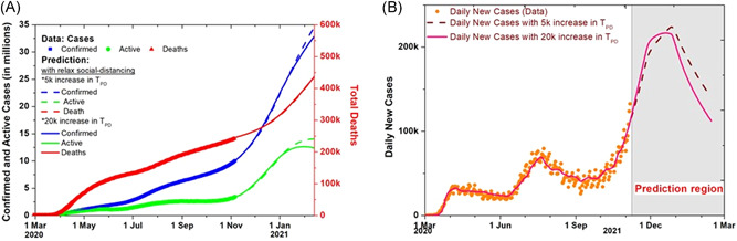
Effect of increased tests and relaxed social distancing. (A) Effect of increased testing on the total, active and extinct cases, comparison of 5000 and 20,000 increase in tests per day (TPD). (B) Model prediction for daily new cases with the increase of 5000 and 20,000 TPD with social distancing conditions relaxed after November 26

The infection to fatality ratio (IFR) is difficult to estimate during the course of the disease spread as the entities in the model are dynamically changing with time. We make a rough estimate by assuming that there is an average delay of 14 days between a person getting infected and becoming extinct.

The initial basic reproduction number for South Korea and Germany turns out to be 3.18 and 3.5, respectively, and for the United States of America, it is 4.8. The South Korea reproduction number by our study is very close to 3.2 reported in Reference [28] and the USA reproduction number is reported as 4.2 on March 16. ² The USA basic reproduction number appears higher than the mean reported value. ²⁹ , ³⁰ However, the IFR calculated with this high initial rate of transmission turns out to be around 0.65%, which is close to the reported value in Reference [25].

A sensitivity study is carried out for the different parameters, as seen in Figures S7 and S8. The parameters are increased and decreased by 10% from the optimized values to see the changes in the outcomes.

4. CONCLUSION

Our findings show that reported cases in the United States of America could only be 35% of the total infected by November 26. If the social distancing is relaxed after November 26, it will lead to around a 47,000 increase in total deaths as compared to having stringent conditions, and doubling the everyday increase in testing from 5000 to 20,000 can reduce this number by 6000. The model prediction shows that in the absence of a vaccine, the infection can spread to around 20% of the total population, and the number of deaths could be around 411,000 if the social distancing conditions remain the same. Our simulation study predicts the future evolution of COVID‐19 in the United States of America for various possible control measures in the coming months, including social distancing conditions and the number of TPD, and thereby provides helpful inputs for policymakers.

CONFLICT OF INTERESTS

The authors declare that there are no conflict of interests.

PEER REVIEW

The peer review history for this article is available at https://publons.com/publon/10.1002/jmv.26897.

Supporting information

Supplementary information.

Mahajan A, Solanki R, Sivadas N. Estimation of undetected symptomatic and asymptomatic cases of COVID‐19 infection and prediction of its spread in the USA. J Med Virol. 2021;93:3202‐3210. 10.1002/jmv.26897

DATA AVAILABILITY STATEMENT

The data that support the findings of this study are openly available at https://www.worldometers.info/coronavirus, https://gis.cdc.gov/grasp/covidnet/COVID19_3.html, https://ourworldindata.org/grapher/full-list-covid19-tests-per-day, and https://covid19.healthdata.org/united-states-ofamerica.

REFERENCES

- 1. Holshue ML, DeBolt C, Lindquist S, et al. First case of 2019 novel coronavirus in the United States. N Engl J Med. 2020;382(10):929‐936. [DOI] [PMC free article] [PubMed] [Google Scholar]
- 2. Gunzler D, Sehgal AR. Time‐varying COVID‐19 reproduction number in the United States. medRxiv. 2020. https://www.medrxiv.org/content/10.1101/2020.04.10.20060863v1 [Google Scholar]
- 3. Anderson RM, May RM. Infectious Diseases of Humans: Dynamics and Control. Oxford, UK: Oxford University Press; 1992. [Google Scholar]
- 4. Brauer F, Castillo‐Chavez C. Mathematical Models in Population Biology and Epidemiology. 2nd ed. New York: Springer; 2012. [Google Scholar]
- 5. Hethcote HW. The mathematics of infectious diseases. SIAM Rev. 2000;42:599‐653. [Google Scholar]
- 6. Diekmann O, Heesterbeek JAP. Mathematical Epidemiology of Infectious Diseases: Model Building, Analysis, and Interpretation. 5th ed. Chichester, UK: John Wiley & Sons; 2000. [Google Scholar]
- 7. Moghadas SM, Shoukat A, Fitzpatrick MC, et al. Projecting hospital utilization during the COVID‐19 outbreaks in the United States. Proc Natl Acad Sci. 2020;117:9122‐9126. [DOI] [PMC free article] [PubMed] [Google Scholar]
- 8. Cavallo JJ, Donoho DA, Forman HP. Hospital Capacity and Operations in the Coronavirus Disease 2019 (COVID‐19) Pandemic—Planning for the Nth Patient. JAMA Health Forum. 2020;1(3):e200345. 10.1001/jamahealthforum.2020.0345 [DOI] [PubMed] [Google Scholar]
- 9. Mizumoto K, Kagaya K, Zarebski A, Chowell G. Estimating the asymptomatic proportion of coronavirus disease 2019 (COVID‐19) cases on board the Diamond Princess cruise ship, Yokohama, Japan, 2020. Euro Surveill. 2020;25:2000180. [DOI] [PMC free article] [PubMed] [Google Scholar]
- 10. Rothe C, Schunk M, Sothmann P, et al. Transmission of 2019‐nCoV infection from an asymptomatic contact in Germany. N Engl J Med. 2020;382:970‐971. [DOI] [PMC free article] [PubMed] [Google Scholar]
- 11. Ogilvy KW, McKendrick AG. A contribution to the mathematical theory of epidemics. Proc R Soc London. 1927;115:700‐721. [Google Scholar]
- 12. Ivorra B, Ramos AM. Application of the Be‐CoDiS mathematical model to forecast the international spread of the 2019–20 Wuhan coronavirus outbreak. ResearchGate Preprints. 2020;9:1–13. [Google Scholar]
- 13. Ivorra B, Ferrández MR, Vela‐Pérez M, Ramos AM. Mathematical modeling of the spread of the coronavirus disease 2019 (COVID‐19) taking into account the undetected infections. The case of China. Communications in Nonlinear Science and Numerical Simulation. 2020;88:105303. 10.1016/j.cnsns.2020.105303 [DOI] [PMC free article] [PubMed] [Google Scholar]
- 14. Giordano G, Blanchini F, Bruno R, et al. A SIDARTHE Model of COVID‐19 epidemic in Italy. arXiv. 2020.2003.09861. [Google Scholar]
- 15. Efimov D, Ushirobira R. On an interval prediction of COVID‐19 development based on a SEIR epidemic model. Ann Rev Control. 2021. 10.1016/j.arcontrol.2021.01.006 [DOI] [PMC free article] [PubMed] [Google Scholar]
- 16. Nande A, Adlam B, Sheen J, Levy MZ, Hill AL. Dynamics of COVID‐19 under social distancing measures are driven by transmission network structure. PLOS Computational Biology. 2021;17(2):e1008684. 10.1371/journal.pcbi.1008684 [DOI] [PMC free article] [PubMed] [Google Scholar]
- 17. Chen Y‐C, Lu P‐E, Chang C‐S, Liu TH. A time‐dependent SIR model for COVID‐19 with undetectable infected persons. arXiv. 2020. 2003.00122. [DOI] [PMC free article] [PubMed] [Google Scholar]
- 18. Zhao S, Lin Q, Ran J, et al. Preliminary estimation of the basic reproduction number of novel coronavirus (2019‐nCoV) in China, from 2019 to 2020: a data‐driven analysis in the early phase of the outbreak. Int J Infect Dis. 2020;92:214‐217. [DOI] [PMC free article] [PubMed] [Google Scholar]
- 19. Zeng T, Zhang Y, Li Z, Liu X, Qui B. Predictions of 2019‐nCov transmission ending via comprehensive methods. arXiv. 2020.2002.04945. [Google Scholar]
- 20. Hu Z, Ge Q, Jin L, Xiong M.Artificial intelligence forecasting of covid‐19 in China. arXiv. 2020.2002.07112. [DOI] [PMC free article] [PubMed] [Google Scholar]
- 21. Murray JLC, IHME COVID . Forecasting the impact of the first wave of the COVID‐19 pandemic on hospital demand and deaths for the USA and European Economic Area countries. medRxiv. 2020. [Google Scholar]
- 22. Mahajan A, Sivadas NA, Solanki R. An epidemic model SIPHERD and its application for prediction of the spread of COVID‐19 infection in India. Chaos Solitons Fractals. 2020;140:110156. [DOI] [PMC free article] [PubMed] [Google Scholar]
- 23. Zhang J, Litvinova M, Wang W, et al. Evolving epidemiology and transmission dynamics of coronavirus disease 2019 outside Hubei province, China: a descriptive and modelling study. Lancet Infect Dis. 2020;20:793‐802. [DOI] [PMC free article] [PubMed] [Google Scholar]
- 24. Garg S, Kim L, Whitaker M, et al. Hospitalization rates and characteristics of patients hospitalized with laboratory‐confirmed coronavirus disease 2019—COVID‐NET, 14 States, March 1–30, 2020. MMWR Morb Mortal Wkly Rep. 2020;69(15):458‐464. [DOI] [PMC free article] [PubMed] [Google Scholar]
- 25. Salje H, Kiem CT, Lefrancq N, et al. Estimating the burden of SARS‐CoV‐2 in France. Science. 2020;369(6500):208‐211. [DOI] [PMC free article] [PubMed] [Google Scholar]
- 26. Novel Coronavirus Pneumonia Emergency Response Epidemiology, others . The epidemiological characteristics of an outbreak of 2019 novel coronavirus diseases (COVID‐19) in China. Zhonghua liu xing bing xue za zhi = Zhonghua liuxingbingxue zazhi. 2020;41:145.32064853 [Google Scholar]
- 27. CDC COVID‐19 Response Team . Severe outcomes among patients with coronavirus disease 2019 (COVID‐19)—United States, February 12–March 16, 2020. MMWR Morb Mortal Wkly Rep. 2020;69:343‐346. [DOI] [PMC free article] [PubMed] [Google Scholar]
- 28. Zhuang Z, Zhao S, Lin Q, Cao P, Lou Y, Yang L, Yang S, He D, Xiao L. Preliminary estimates of the reproduction number of the coronavirus disease (COVID‐19) outbreak in Republic of Korea and Italy by 5 March 2020. International Journal of Infectious Diseases. 2020;95:308–310. 10.1016/j.ijid.2020.04.044 [DOI] [PMC free article] [PubMed] [Google Scholar]
- 29. Liu Y, Gayle AA, Wilder‐Smith A, Rocklöv J. The reproductive number of COVID‐19 is higher compared to SARS coronavirus. J Travel Med. 2020;27(2):taaa021. [DOI] [PMC free article] [PubMed] [Google Scholar]
- 30. Read JM, Bridgen JRE, Cummings DAT, Ho A, Jewell CP. Novel coronavirus 2019‐nCoV: early estimation of epidemiological parameters and epidemic predictions. MedRxiv. 2020. [DOI] [PMC free article] [PubMed] [Google Scholar]
Associated Data
This section collects any data citations, data availability statements, or supplementary materials included in this article.
Supplementary Materials