A case study of Covid‐19 epidemic in India via new generalised Caputo type fractional derivatives

Abstract

The first symptomatic infected individuals of coronavirus (Covid‐19) was confirmed in December 2020 in the city of Wuhan, China. In India, the first reported case of Covid‐19 was confirmed on 30 January 2020. Today, coronavirus has been spread out all over the world. In this manuscript, we studied the coronavirus epidemic model with a true data of India by using Predictor‐Corrector scheme. For the proposed model of Covid‐19, the numerical and graphical simulations are performed in a framework of the new generalised Caputo sense non‐integer order derivative. We analysed the existence and uniqueness of solution of the given fractional model by the definition of Chebyshev norm, Banach space, Schauder's second fixed point theorem, Arzel's‐Ascoli theorem, uniform boundedness, equicontinuity and Weissinger's fixed point theorem. A new analysis of the given model with the true data is given to analyse the dynamics of the model in fractional sense. Graphical simulations show the structure of the given classes of the non‐linear model with respect to the time variable. We investigated that the mentioned method is copiously strong and smooth to implement on the systems of non‐linear fractional differential equation systems. The stability results for the projected algorithm is also performed with the applications of some important lemmas. The present study gives the applicability of this new generalised version of Caputo type non‐integer operator in mathematical epidemiology. We compared that the fractional order results are more credible to the integer order results.

1. INTRODUCTION

Novel coronavirus or 2019‐nCoV (Covid‐19), a dangerous pandemic disease, is firstly detected in the city of Wuhan, China in December 2019. ¹ , ² Today, so many countries are suffering from this virus all over the world. From its starting date, it rapidly increased in the population and affected more than 21,095,532 with 757,779 deaths and 13,946,466 recoveries on August 14 all over the globe. Coronaviruses are a large family of viruses, and a novel coronavirus is a new strain in this family that has not been recognised before. Coronaviruses are transmitted between people and animals. But still several coronaviruses are circulating in animals and yet not infected to the humans. Breathing difficulties, cough and fever are the most common symptoms of this virus. In India, the first reported case of Covid‐19 was confirmed on 30 January 2020 in Thrissur district of Kerala and there are 2,594,112 reported cases with 50,122 deaths and 1,862,937 recoveries has been recorded till 16 August 2020. India is the second largest population country and now the third most infected country by this virus on 16 August 2020. Indian government enforced a strict lockdowns and also suspended all the tourist visas to control the spread of this virus. Some of the countries that strongly commanded the pandemic including Iceland, New Zealand, Fiji, Tanzania, Montenegro, Vatican city, Papua New Guinea, Seychelles and Mauritius. On February 28, 2020, New Zealand founded its first Covid‐19 patient and then applied one of the toughest lockdown in the world. Lots of research studies have been done to investigate the outbreaks of coronavirus via mathematical modelling. ³ , ⁴ , ⁵ In Nabi et al., ⁶ authors analysed the Covid‐19 cases in Cameroon via integer and non‐integer order derivatives. A time‐delay fractional dynamical model of Covid‐19 has studied by the researchers in Kumar and Suat Erturk. ⁷ q‐homotopy analysis transform technique experimented on a non‐linear mathematical model of coronavirus in Gao et al. ⁸

Fractional Calculus (non‐classical Calculus) is the part of applied mathematics implants the theory of fractional derivatives and differential equations. The literature of fractional calculus is more than 350+ years chronic. Continuously a big amount of new theory is being added in this Calculus. In Rashid et al., ⁹ authors proposed some new capaciousness for non‐integer order integral operator in the sense of exponential type kernel and given their uses in physical systems. In Rashid et al., ¹⁰ a research study on descent of new non‐integer order inequalities in the framework of n polynomials s‐type convexity with praxis has analysed. Khan et al. ¹¹ organised a study related to generalized trapezium‐type inequalities in the fiddlestick of fractal sets for mappings having generalized convexity merits. Nikan et al. ¹² give some analysis on numerical simulations of the non‐integer order evolution model framework for heat flow in projections with memory. Some new multi‐parametrized evolutions containing pth‐order differentiability in non‐integer order Calculus for effecting h‐Convex mappings in Hilbert space are given in Rashid et al. ¹³ Some inequalities in the sense of generalized proportional non‐integer order integral operators with the support of another function proposed in Rashid et al. ¹⁴ Number of various types of non‐integer order derivatives have been suggested by the researchers and used in different branches of scientific and engineering fields. ¹⁵ , ¹⁶ , ¹⁷ , ¹⁸ , ¹⁹ Caputo, Caputo and Fabrizio (CF) and Atangana‐Baleanu‐Caputo (ABC) derivatives are the most famous operators applied in the different scientific fields. Caputo derivative is defined with non local but singular kernel (power law type), Caputo‐Fabrizio with non‐singular kernel (exponentially decaying type) and AB derivative with Mittag‐ Leffler type kernel. Lately, a new generalised version of Caputo type non‐integer derivative which has the properties similar to Caputo derivatives introduced by Odibat et al. ²⁰ An analysis on the asymptotic stability of generalised Caputo type non‐integer order differential equations has been done in Baleanu et al. ²¹ In the literature, so many articles have been given to study the epidemiological models via well known fractional derivatives. A model to describe the Chickenpox disease with the real data of China has been successfully studied via Caputo to AB derivative in Qureshi and Yusuf. ²² In Kumar et al., ²³ authors solved a malaria disease model via Caputo‐Fabrizio and Atangana‐Baleanu non‐integer order derivatives. In Kumar and Erturk, ²⁴ authors proposed an ecological study via fractional derivatives. A mathematical modelling of Ebola virus with an efficient technique in fractional sense is studied by Muhammad Altaf and Atangana. ²⁵ A non‐classical structure of population model is described in Rivero et al. ²⁶ Human immunodeficiency virus (HIV) dynamics in both ordinary and non‐integer sense is analysed with local asymptotic stability results in Babaei et al. ²⁷ and Babaei et al., ²⁸ respectively. Lastly, there are some new techniques introduced by mathematicians to find the solution of non‐linear non‐integer order differential equations. A new method to solve non‐linear integro‐differential equations of volterra type in Atangana‐Baleanu sense is generated in Ganji and Jafari. ²⁹ An another method for the fractional differential equations based on Genocchi polynomials is proposed in Sadeghi et al. ³⁰ One more new algorithm to investigate more than one variable order differential equations in AB derivative sense is suggested by Ganji et al. ³¹ Memory effects and crossover behaviour of the model are the important advantages of the uses of non‐integer order derivatives. By the fractional operators, we can compare the true data more clearly to the model outputs respect to the time variable. There are so many cases when we see that the complex structures that can not be analysed clearly by ordinary derivatives can be study by fractional derivatives more smoothly. In the features of the new generalised Caputo non‐integer derivative, the parameter ρ plays a considerable role. We can generate more diversities in the graphs by the help of this parameter ρ which is an advantage of using this newly proposed derivative. Also there are some finishing points in the non‐integer order calculus. In many conditions, the existence of fractional dynamics solution can not be smoothly analysed. Recently, a lot of research articles are come to this area to prove the solutions existence of FDEs. Recently, an existence study for infinite coefficient symmetric integro‐differential equations in Caputo‐Fabrizio sense is analysed by Baleanu et al. ³²

The major goal of this research study is to analyse the non‐integer order coronavirus pandemic model by the help of new generalised Caputo fractional derivative with Predictor‐Corrector method. The paper is prepared as follows. In Section 2, we give some necessary definitions of fractional derivatives. Section 3 is given for the complete knowledge of the ODE model following by the non‐integer order model. Results for the proof of existence of unique solution of the given model are analysed in Section 4. Projected model is solved in Section 5. All necessary simulation results are discussed in Section 6. At the last, we have given a conclusion.

2. PRELIMINARIES

Here, we give some important definitions and results related to generalized fractional derivatives.

Definition 1

(Podlubny ¹⁸ ) The Caputo type fractional derivative of $F\in C_{-1}^k$ is presented as

$$D_{\zeta }^{\theta }F(\zeta )=\left\{\begin{array}{ll}\frac{d^{k}F(\zeta )}{d{\zeta }^k},& \theta =k\in \mathbb{N}\\ \frac{1}{\mathrm{\Gamma }(k-\theta )}{\int }_0^{\zeta }{\left(\zeta -\vartheta \right)}^{k-\theta -1}{F}^{(k)}(\vartheta )d\vartheta ,& k-1<\theta <k,k\in \mathbb{N}.\end{array}\right.$$ (1)

Definition 2

(Katugampola ³³ ) The generalized Riemann‐type non‐integer order derivative, ${}^R{D}_{c_{+}}^{\theta ,\rho }$, of order θ > 0 is expressed as

$$({}^R{D}_{c_{+}}^{\theta ,\rho }g)(\eta )=\frac{{\rho }^{\theta -n+1}}{\mathrm{\Gamma }(n-\theta )}{\left({\eta }^{1-\rho }\frac{d}{d\eta }\right)}^n{\int }_c^{\eta }{s}^{\rho -1}{({\eta }^{\rho }-s^{\rho })}^{n-\theta -1}g(s)ds,\eta >c,$$ (2)

where ρ > 0, c ≥ 0,  and n − 1 < θ ≤ n .

Definition 3

(Katugampola ³³ ) The generalized version of Caputo fractional derivative, ${}^C{D}_{c_{+}}^{\theta ,\rho }$, of order θ > 0 is defined as

$$({}^C{D}_{c_{+}}^{\theta ,\rho }g)(\eta )=\left({}^R{D}_{c_{+}}^{\theta ,\rho }\left[g(x)-{\displaystyle \sum _{m=0}^{n-1}}\frac{g^{(m)}(c)}{m!}{(x-c)}^m\right]\right)(\eta ),\eta >c,$$ (3)

where $\rho >0,c\ge 0,andn=\lceil \theta \rceil$.

Definition 4

(Odibat and Baleanu ²⁰ ) The new generalized form of the Caputo‐type non‐integer order derivative, $D_{c_{+}}^{\theta ,\rho }$, of order θ > 0 is expressed as

$$(D_{c_{+}}^{\theta ,\rho }g)(\eta )=\frac{{\rho }^{\theta -n+1}}{\mathrm{\Gamma }(n-\theta )}{\int }_c^{\eta }{s}^{\rho -1}{({\eta }^{\rho }-s^{\rho })}^{n-\theta -1}{\left(s^{1-\rho }\frac{d}{ds}\right)}^{n}g(s)ds,\eta >c,$$ (4)

where ρ > 0, c ≥ 0,  and n − 1 < θ ≤ n .

Lemma 1

(Li and Zeng ³⁴ ) If 0 < η < 1 and k is an nonnegative integer, then the positive constants ${\mathcal{C}}_{\eta ,1}$ and ${\mathcal{C}}_{\eta ,2}$ exists and only dependent on η , s.t

$${(k+1)}^{\eta }-k^{\eta }\le {\mathcal{C}}_{\eta ,1}{(k+1)}^{\eta -1},$$

and

$${(k+2)}^{\eta +1}-2{(k+1)}^{\eta +1}+k^{\eta +1}\le {\mathcal{C}}_{\eta ,2}{(k+1)}^{\eta -1}.$$

Lemma 2

(Li and Zeng ³⁴ ) Assume that $d_{q,s}={(s-q)}^{\eta -1}(q=\mathrm{1,2},\dots ,s-1)$ & $d_{q,s}=0$ for q ≥ s, η, M, h, T > 0, rh ≤ T & r is a positive integer. Let ${\sum }_{q=r}^{q=s}{d}_{q,s}|e_q|=0$ for k > s ≥ 1. If

$$|e_s|\le M{h}^{\eta }{\displaystyle \sum _{q=1}^{s-1}}{d}_{q,s}|e_q|+|{\beta }_0|,s=\mathrm{1,2},\dots ,r,$$

then

$$|e_r|\le \mathcal{C}|{\beta }_0|,r=\mathrm{1,2},\dots$$

where $\mathcal{C}$ is a positive constant not dependent on r & h.

3. MODEL EXPLANATION

In this section, we analyse the ordinary model introduced by Sarkar et al. ³⁵ to study the coronavirus pandemic in India. The given model structured of six classes with population of susceptible S(t), quarantined susceptible population S _q (t), asymptomatic infectious individuals A(t), infectious I(t), isolated infected individuals I _q (t) and recovered R(t). The author investigated and defined the dynamical model in the ordinary differential equations sense as follows:

$$\begin{array}{ccc}\hfill S^{\prime }(t)& ={\mathrm{\Lambda }}_s-({\beta }_s+{\gamma }_s(1-{\beta }_s)){\mu }_s\frac{SI}{N}-ϵS+u_s{S}_q,\hfill & \hfill \\ \hfill S_q^{\prime }(t)& ={\gamma }_s(1-{\beta }_s){\mu }_s\frac{SI}{N}-(u_s+ϵ)S_q\hfill \\ \hfill A^{\prime }(t)& ={\beta }_s(1-{\gamma }_s){\mu }_s\frac{SI}{N}-({\delta }_a+{\xi }_a+ϵ)A,\hfill \\ \hfill I^{\prime }(t)& ={\delta }_{a}A-({\delta }_i+{\xi }_i+ϵ)I,\hfill \\ \hfill I_q^{\prime }(t)& ={\beta }_s{\mu }_s{\gamma }_s\frac{SI}{N}+{\delta }_{i}I-({\xi }_q+ϵ)I_q,\hfill \\ \hfill R^{\prime }(t)& ={\xi }_{a}A+{\xi }_{i}I+{\xi }_q{I}_q-ϵR.\hfill \end{array}$$ (5)

with the basic reproductive number

$${\mathcal{R}}_0=\frac{{\beta }_s(1-{\gamma }_s){\mu }_s{\delta }_a}{({\delta }_a+{\xi }_a)({\delta }_i+{\xi }_i)}.$$ (6)

The re‐formulation of the above model (5) in the new generalised Caputo type non‐integer derivative sense is as follows:

$$\left\{\begin{array}{cc}{}^C{D}_t^{\theta ,\rho }S(t)& ={\mathrm{\Lambda }}_s-({\beta }_s+{\gamma }_s(1-{\beta }_s)){\mu }_s\frac{SI}{N}-ϵS+u_s{S}_q,\\ {}^C{D}_t^{\theta ,\rho }{S}_q(t)& ={\gamma }_s(1-{\beta }_s){\mu }_s\frac{SI}{N}-(u_s+ϵ)S_q,\\ {}^C{D}_t^{\theta ,\rho }A(t)& ={\beta }_s(1-{\gamma }_s){\mu }_s\frac{SI}{N}-({\delta }_a+{\xi }_a+ϵ)A,\\ {}^C{D}_t^{\theta ,\rho }I(t)& ={\delta }_{a}A-({\delta }_i+{\xi }_i+ϵ)I,\\ {}^C{D}_t^{\theta ,\rho }{I}_q(t)& ={\beta }_s{\mu }_s{\gamma }_s\frac{SI}{N}+{\delta }_{i}I-({\xi }_q+ϵ)I_q,\\ {}^C{D}_t^{\theta ,\rho }R(t)& ={\xi }_{a}A+{\xi }_{i}I+{\xi }_q{I}_q-ϵR.\end{array}\right.$$ (7)

where ${}^C{D}_t^{\theta ,\rho }$ denotes the new generalised Caputo fractional derivative operator.

The equivalent compact form of the given fractional system (7) is as follows:

$$\left\{\begin{array}{cc}{}^C{D}_t^{\theta ,\rho }S(t)& ={\mathcal{G}}_1(t,S(t)),\\ {}^C{D}_t^{\theta ,\rho }{S}_q(t)& ={\mathcal{G}}_2(t,S_q(t)),\\ {}^C{D}_t^{\theta ,\rho }A(t)& ={\mathcal{G}}_3(t,A(t)),\\ {}^C{D}_t^{\theta ,\rho }I(t)& ={\mathcal{G}}_4(t,I(t)),\\ {}^C{D}_t^{\theta ,\rho }{I}_q(t)& ={\mathcal{G}}_5(t,I_q(t)),\\ {}^C{D}_t^{\theta ,\rho }R(t)& ={\mathcal{G}}_6(t,R(t)).\end{array}\right.$$ (8)

with the initial population classes taken as $S(0)=S_0,S_q(0)=S_{q_0},A(0)=A_0,I(0)=I_0,I_q(0)=I_{q_0}$ and $R(0)=R_0$.

4. FRACTIONAL ANALYSIS OF THE GIVEN MODEL

4.1. Existence of unique solution

In this portion of study, we do the existence and uniqueness analysis of the given Covid‐19 model by the applications of the results of fixed point results. We do the investigations for the first equation of system (8) and it is worthwhile to say that for remaining equations of the system these analysis will be similar. Now define the initial value problem (IVP)

$${}^C{D}_t^{\theta ,\rho }S(t)={\mathcal{G}}_1(t,S),$$ (9a)

$$S(0)=S_0.$$ (9b)

The Volterra integral equation (VIE) similar to the above IVP is

$$S(t)=S(0)+\frac{{\rho }^{1-\theta }}{\mathrm{\Gamma }(\theta )}{\int }_0^t{\chi }^{\rho -1}{(t^{\rho }-{\chi }^{\rho })}^{\theta -1}{\mathcal{G}}_1(\chi ,S)d\chi ,$$ (10)

Now, first to do the analysis for the existence of solution we are going as follows.

Theorem 1

(Existence) Let $0<\theta \le 1,S_0\in ℝ,J>0$ and T ^∗ > 0. Demarcate $\mathcal{G}:=\{(t,S):t\in [0,T^{\ast }],|S-S_0|\le J\}$ and define the mapping ${\mathcal{G}}_1:\mathcal{G}\to ℝ$ be continuous. Also, let $M:={\sup }_{(t,S)\in \mathcal{G}}|{\mathcal{G}}_1(t,S)|$ and

$$T=\left\{\begin{array}{cl}{T}^{\ast },& ifM=0,\\ min\left\{T^{\ast },{\left(\frac{J\mathrm{\Gamma }(\theta +1){\rho }^{\theta }}{M}\right)}^{\frac{1}{\theta }}\right\}& otherwise.\end{array}\right.$$ (11)

Then, there exists a function $S\in \mathcal{C}[0,T]$ that satisfy the IVP (9a) and (9b).

Lemma 3

(Katugampola ³³ ) Assuming the statement of Theorem 1, the function $S\in \mathcal{C}[0,T]$ is satisfy the initial value problem (9a) and (9b) iff, it satisfies the Volterra integral Equation (10).

(Theorem 1 Proof) When $M=0$ then ${\mathcal{G}}_1(t,S)=0$ for all $(t,S)\in \mathcal{G}$. In that condition by the straight substitution it is clear that the function $S:[0,T]\to ℝ$ with $S(t)=S_0$ become a solution of the initial value problem. Hence in this case a solution rises.

Now when M ≠ 0, we use Lemma (3) and show that the IVP (9a) and (9b) is similar to the VIE (10). Demarcate the set $\mathcal{E}:=\{S\in \mathcal{C}[0,T]:\Vert S-S_0{\Vert }_{\infty }\le J\}$. It is straight that $\mathcal{E}$ is a convex and closed subset of the Banach space of all functions of continuous family on [0, T], furnished with the Chebyshev type norm. So, $\mathcal{E}$ is a Banach space and non empty, since $S_0\in \mathcal{E}$. We derive the operator $\mathcal{F}$ on the set $\mathcal{E}$ by

$$(\mathcal{F}S)(t):=S(0)+\frac{{\rho }^{1-\theta }}{\mathrm{\Gamma }(\theta )}{\int }_0^t{\chi }^{\rho -1}{(t^{\rho }-{\chi }^{\rho })}^{\theta -1}{\mathcal{G}}_1(\chi ,S)d\chi .$$ (12)

So, now the Volterra integral Equation (10) can be described as $S=\mathcal{F}S$ and thus, we have to prove that $\mathcal{F}$ has a fixed point. This is performed by the Schauder's Second Fixed Point result. We first prove that $\mathcal{E}$ is closed, that is, $\mathcal{F}S\in \mathcal{E}$ for $S\in \mathcal{E}$. We start by considering that, for 0 ≤ t ₁ ≤ t ₂ ≤ T ,

$$\begin{array}{ccc}\hfill & |(\mathcal{F}S)(t_1)-(\mathcal{F}S)(t_2)|=\frac{{\rho }^{1-\theta }}{\mathrm{\Gamma }(\theta )}\left|{\int }_0^{t_1}{\chi }^{\rho -1}{(t_1^{\rho }-{\chi }^{\rho })}^{\theta -1}{\mathcal{G}}_1(\chi ,S)d\chi -{\int }_0^{t_2}{\chi }^{\rho -1}{(t_2^{\rho }-{\chi }^{\rho })}^{\theta -1}{\mathcal{G}}_1(\chi ,S)d\chi \right|\hfill & \hfill \\ \hfill & =\frac{{\rho }^{1-\theta }}{\mathrm{\Gamma }(\theta )}\left|{\int }_0^{t_1}[{(t_1^{\rho }-{\chi }^{\rho })}^{\theta -1}-{(t_2^{\rho }-{\chi }^{\rho })}^{\theta -1}]{\chi }^{\rho -1}{\mathcal{G}}_1(\chi ,S)d\chi +{\int }_{t_1}^{t_2}{\chi }^{\rho -1}{(t_2^{\rho }-{\chi }^{\rho })}^{\theta -1}{\mathcal{G}}_1(\chi ,S)d\chi \right|\hfill \\ \hfill & \le \frac{M{\rho }^{1-\theta }}{\mathrm{\Gamma }(\theta )}\left({\int }_0^{t_1}|{(t_1^{\rho }-{\chi }^{\rho })}^{\theta -1}-{(t_2^{\rho }-{\chi }^{\rho })}^{\theta -1}|{\chi }^{\rho -1}d\chi +{\int }_{t_1}^{t_2}{\chi }^{\rho -1}{(t_2^{\rho }-{\chi }^{\rho })}^{\theta -1}d\chi \right)\hfill \end{array}$$

The second integral part value present in the right side of the last inequality is $\frac{1}{\rho \theta }{(t_2^{\rho }-{\chi }^{\rho })}^{\theta }$. For the first integral, analyse the two conditions $\theta <1,\theta =1$, aside. In the condition $\theta =1$, the value of the integral is zero. For θ < 1, we have ${(t_1^{\rho }-{\chi }^{\rho })}^{\theta -1}\ge {(t_2^{\rho }-{\chi }^{\rho })}^{\theta -1}$. Thus,

$$\begin{array}{ccc}\hfill & {\int }_0^{t_1}|{(t_1^{\rho }-{\chi }^{\rho })}^{\theta -1}-{(t_2^{\rho }-{\chi }^{\rho })}^{\theta -1}|{\chi }^{\rho -1}d\chi ={\int }_0^{t_1}[{(t_1^{\rho }-{\chi }^{\rho })}^{\theta -1}-{(t_2^{\rho }-{\chi }^{\rho })}^{\theta -1}]{\chi }^{\rho -1}d\chi \hfill & \hfill \\ \hfill & =\frac{1}{\rho \theta }(t_1^{\rho }\theta -t_2^{\rho }\theta )+\frac{1}{\rho \theta }{(t_2^{\rho }-t_1^{\rho })}^{\theta }\hfill \\ \hfill & \le \frac{1}{\rho \theta }{(t_2^{\rho }-t_1^{\rho })}^{\theta }.\hfill \end{array}$$

Combining these results, we have

$$|(\mathcal{F}S)(t_1)-(\mathcal{F}S)(t_2)|\le \frac{2M}{{\rho }^{\theta }\mathrm{\Gamma }(\theta +1)}{(t_2^{\rho }-t_1^{\rho })}^{\theta }$$ (13)

if θ ≤ 1. In the other case, the description on the right‐hand part of (13) goes to 0 as t ₂ → t ₁ , which gives that $\mathcal{F}S$ is a continuous mapping, since S(0) continuous itself. It is also correct that for $S\in \mathcal{E}$ and t ∈ [0, T],

$$\begin{array}{ccc}\hfill & |(\mathcal{F}S)(t)-S(0)|=\frac{{\rho }^{1-\theta }}{\mathrm{\Gamma }(\theta )}\left|{\int }_0^t{\chi }^{\rho -1}{(t^{\rho }-{\chi }^{\rho })}^{\theta -1}{\mathcal{G}}_1(\chi ,S)d\xi \right|\hfill & \hfill \\ \hfill & \le \frac{M}{{\rho }^{\theta }\mathrm{\Gamma }(\theta +1)}{t}^{\rho \theta }\le \frac{M}{{\rho }^{\theta }\mathrm{\Gamma }(\theta +1)}{T}^{\rho \theta }\hfill \\ \hfill & \le \frac{M}{{\rho }^{\theta }\mathrm{\Gamma }(\theta +1)}.\frac{{\rho }^{\theta }J\mathrm{\Gamma }(\theta +1)}{M}=J.\hfill \end{array}$$ (14)

by the description of T. Thus, we have $\mathcal{F}S\in \mathcal{E}$ if $S\in \mathcal{E}$, i.e., $\mathcal{F}$ projects the set $\mathcal{E}$ into itself. Now we just have to prove that $\mathcal{F}(\mathcal{E}):=\{\mathcal{F}u:u\in \mathcal{E}\}$ is relatively compact, which is become complete by the application of Arzel‘a‐Ascoli Theorem. To give that the set $\mathcal{F}(\mathcal{E})$ is bounded uniformly, assume $z\in \mathcal{F}(\mathcal{E})$. We analyse that, ∀  t ∈ [0, T],

$$|z(t)|=|(\mathcal{F}S)(t)|$$

$$\le {\Vert S(0)\Vert }_{\infty }+\frac{{\rho }^{1-\theta }}{\mathrm{\Gamma }(\theta )}{\int }_0^t{\chi }^{\rho -1}{(t^{\rho }-{\chi }^{\rho })}^{\theta -1}|{\mathcal{G}}_1(\chi ,S)|d\chi$$

$$\le {\Vert S(0)\Vert }_{\infty }+\frac{1}{{\rho }^{\theta }\mathrm{\Gamma }(\theta +1)}M{T}^{\theta }\le {\Vert S(0)\Vert }_{\infty }+J,$$

which is the expected property of boundedness. The equicontinuity characteristic can be analysed smoothly from (13) above. For 0 ≤ t ₁ ≤ t ₂ ≤ T , we proved in the case θ ≤ 1 that

$$|(\mathcal{F}S)(t_1-t_2)|\le \frac{2M}{{\rho }^{\theta }\mathrm{\Gamma }(\theta +1)}{(t_2^{\rho }-t_1^{\rho })}^{\theta }.$$

After analysing the Mean Value Theorem and the Triangle Inequality, we received

$$|(\mathcal{F}S)(t_1)-(\mathcal{F}S)(t_2)|\le \frac{2M}{{\rho }^{\theta }\mathrm{\Gamma }(\theta +1)}{(t_2^{\rho }-t_1^{\rho })}^{\theta }.$$

$$=\frac{2M}{\mathrm{\Gamma }(\theta +1)}{(t_2-t_1)}^{\theta }{\gamma }^{\theta (\rho -1)}$$

for some γ ∈ [t ₁, t ₂] ⊂ [0, T]. Thus, if |t ₂ − t ₁|<δ , we have

$$|(\mathcal{F}S)(t_1)-(\mathcal{F}S)(t_2)|\le M^{\prime }\delta +\frac{2M}{\mathrm{\Gamma }(\theta +1)}{\delta }^{\theta }{T}^{\theta (\rho -1)}.$$

for some M ′ > 0, since in the given closed interval [0, T], S(0) is uniformly continuous. We see that the equation on the right side is not dependent on S,  t ₁ and t ₂ , we analyse that the set $\mathcal{F}(\mathcal{E})$ equicontinous. In other case, the Arzel‘a‐Ascoli Theorem gives that $\mathcal{F}(\mathcal{E})$ is relatively compact, and hence $\mathcal{F}$ has a fixed point asserted by Schauder’s second Fixed Point Theorem. This fixed point is the undersigned solution of the IVP (9a) and (9b). This is the end of the proof.

Now to do the analysis for the uniqueness of the solution. In starting we detect the characteristic of the operator $\mathcal{F}$(given in (12)). Thus, let $S_1,S_2\in \mathcal{C}[0,T]\subset [0,t]$ and let there exists a constant V > 0 not dependent of t, S ₁ and S ₂ such that $|{\mathcal{G}}_1(t,S_1)-{\mathcal{G}}_2(t,S_2)|\le V|S_1-S_2|$ for all t ∈ [0, T]. Then we have

$$\begin{array}{ccc}\hfill & {\Vert \mathcal{F}{S}_1-\mathcal{F}{S}_2\Vert }_{V_{\infty }[0,t]}=\frac{{\rho }^{1-\theta }}{\mathrm{\Gamma }(\theta )}\underset{0\le \omega \le t}{\sup }\left|{\int }_0^{\omega }{({\omega }^{\rho }-{\chi }^{\rho })}^{\theta -1}{\chi }^{\rho -1}[{\mathcal{G}}_1(\chi ,S_1(\chi ))-{\mathcal{G}}_1(\chi ,S_2(\chi ))]d\chi \right|\hfill & \hfill \\ \hfill & \le \frac{V{\rho }^{1-\theta }}{\mathrm{\Gamma }(\theta )}\underset{0\le \omega \le t}{\sup }\left|{\int }_0^{\omega }{({\omega }^{\rho }-{\chi }^{\rho })}^{\theta -1}{\chi }^{\rho -1}\right|S_1(\chi )-S_2(\chi )|d\chi |\hfill \\ \hfill & \le \frac{V{\rho }^{1-\theta }}{\mathrm{\Gamma }(\theta )}{\Vert S_1-S_2\Vert }_{V_{\infty }[0,t]}\underset{0\le \omega \le t}{\sup }\left|{\int }_0^{\omega }{({\omega }^{\rho }-{\chi }^{\rho })}^{\theta -1}{\chi }^{\rho -1}d\chi \right|\hfill \\ \hfill & \le \frac{V{\rho }^{1-\theta }}{\mathrm{\Gamma }(\theta )}{\Vert S_1-S_2\Vert }_{V_{\infty }[0,t]}\underset{0\le \omega \le t}{\sup }\left|\frac{1}{\rho \theta }{({\omega }^{\rho }-{\chi }^{\rho })}^{\theta }{|}_0^{\omega }\right|\hfill \\ \hfill & =\frac{V{\left(\frac{t^{\rho }}{\rho }\right)}^{\theta }}{\mathrm{\Gamma }(1+\theta )}{\Vert S_1-S_2\Vert }_{L_{\infty }[0,t]}.\hfill \end{array}$$

Next, in this regard we have the results given blow;

Theorem 2

(Katugampola ³³ ) Let $\mathcal{F}$ and $\mathcal{E}$ be expressed as in Theorem 1. Also let $j\in {\mathbb{N}}_0,t\in [0,T]andS,\tilde{S}\in \mathcal{E}$. Suppose ${\mathcal{G}}_1$ agrees the Lipschitz condition with the constant V. Then

$${\Vert {\mathcal{F}}^{j}S-{\mathcal{F}}^j\tilde{S}\Vert }_{V_{\infty }[0,t]}\le \frac{V^j{\left(\frac{t^{\rho }}{\rho }\right)}^{\theta j}}{\mathrm{\Gamma }(1+\theta j)}{\Vert S-\tilde{S}\Vert }_{V_{\infty }[0,t]}.$$ (15)

Theorem 3

(Result for Uniqueness) Assume $S(0)\in ℝ,J>0and{T}^{\ast }>0$. Further assume $0<\theta \le 1andm=\lceil \theta \rceil$. Derive the set $\mathcal{G}$ given in Theorem 1 and put the continuous mapping ${\mathcal{G}}_1:\mathcal{G}\to ℝ$ and agrees a Lipschitz condition regards to the second variable, i.e.

$$|{\mathcal{G}}_1(t,S_1)-{\mathcal{G}}_1(t,S_2)|\le V|S_1-S_2|$$

for some constant V > 0 not dependent on t, S ₁,  and S ₂ . Then, a unique solution $S\in \mathcal{C}[0,T]$ exists for the initial value problem (9a) and (9b).

By the Theorem 1, the problem (9a) and (9b) has a solution. In the way to prove the uniqueness of solution, we use Theorem 2. Separately, we take the operator $\mathcal{F}$ as given in (12) and remind that it projects the nonempty, closed and convex set $\mathcal{E}=\{S\in \mathcal{C}[0,T]:{\Vert S-S_0\Vert }_{\infty }\le J\}$ to the same. We use Weissinger's Fixed Point Theorem to give that $\mathcal{F}$ has a unique fixed point. Assume $j\in {\mathbb{N}}_0,t\in [0,T]and{S}_1,S_2\in \mathcal{E}$. Then, using (15) and taking the Chebyshev type norm on the range [0, T], we receive

$${\Vert {\mathcal{F}}^{j}S-{\mathcal{F}}^j\tilde{S}\Vert }_{\infty }\le \frac{V^j{\left(\frac{t^{\rho }}{\rho }\right)}^{\theta j}}{\mathrm{\Gamma }(1+\theta j)}{\Vert S-\tilde{S}\Vert }_{\infty }.$$

Let ${\omega }_j=V^j{(T^{\rho }/\rho )}^{\theta j}/\mathrm{\Gamma }(1+\theta j)$. In the way to use the theorem, we only require to clarify that the series ${\displaystyle \sum _{j=0}^{\infty }}{\omega }_j$ converges. It is apparent from analysing that ω _j is just the power series expression of the Mittag‐Leffler type function $E_{\theta }^{\ast }(V{(T^{\rho }/\rho )}^{\theta })$ hence the series converges. This is the end of the proof.

5. MODEL SOLUTION BY THE HELP OF MODIFIED PREDICTOR‐CORRECTOR SCHEME

In this section, we establish the numerical solution of the given model (8) with the application of Predictor‐Corrector method. We adhere the same methodology as given in Odibat and Baleanu ²⁰ with some changes, and then, we do the stability analysis of this numerical technique with the uses of some necessary lemmas. For this purpose, first we construct the solution for the first equation of (8) and then we will write the corrector and predictor formula for each equations of system (8). The compeer VIE of first equation of the model (8) is

$$S(t)=S(0)+\frac{{\rho }^{1-\theta }}{\mathrm{\Gamma }(\theta )}{\int }_0^t{\chi }^{\rho -1}{(t^{\rho }-{\chi }^{\rho })}^{\theta -1}{\mathcal{G}}_1(\chi ,S)d\chi ,$$ (16)

The starting concern of the method, under the reminder of the unique solution existence of the given function ${\mathcal{G}}_1$ on the interval [0, T], exists of splitting the interval [0, T] into N disparate subintervals $\{[t_r,t_{r+1}],r=\mathrm{0,1},\dots ,N-1\}$ taking the mesh points

$$\left\{\begin{array}{c}{t}_0=0,\\ t_{r+1}={(t_r^{\rho }+h)}^{1/\rho },r=\mathrm{0,1},\dots ,N-1,\end{array}\right.$$ (17)

where $h=\frac{T^{\rho }}{N}$. Now, trying to find the approximations $S_r,r=\mathrm{0,1},\dots ,N$, to solve the IVP (9a). The general step, supposing that we have calculated the approximations $S_j\approx S(t_j)(j=\mathrm{1,2},\dots ,r)$, and now desire to find the approximation S _r + 1 ≈ S(t _r + 1) by the regards of the equation

$$S(t_{r+1})=S(0)+\frac{{\rho }^{1-\theta }}{\mathrm{\Gamma }(\theta )}{\int }_0^{t_{r+1}}{\chi }^{\rho -1}{(t_{r+1}^{\rho }-{\chi }^{\rho })}^{\theta -1}{\mathcal{G}}_1(\chi ,S)d\chi ,$$ (18)

doing the substitution $z={\chi }^{\rho }$, we receive

$$S(t_{r+1})=S(0)+\frac{{\rho }^{-\theta }}{\mathrm{\Gamma }(\theta )}{\int }_0^{t_{r+1}^{\rho }}{(t_{r+1}^{\rho }-z)}^{\theta -1}{\mathcal{G}}_1(z^{1/\rho },S(z^{1/\rho }))dz.$$ (19)

That is

$$S(t_{r+1})=S(0)+\frac{{\rho }^{-\theta }}{\mathrm{\Gamma }(\theta )}{\displaystyle \sum _{j=0}^r}{\int }_{t_j^{\rho }}^{t_{r+1}^{\rho }}{(t_{r+1}^{\rho }-z)}^{\theta -1}{\mathcal{G}}_1(z^{1/\rho },S(z^{1/\rho }))dz.$$ (20)

Next, in the theme of the weight function ${(t_{r+1}^{\rho }-z)}^{\theta -1}$ if we harness the trapezoidal quadrature rule to analyse the integrals take a form in the right‐hand side of Equation (20), changing the function ${\mathcal{G}}_1(z^{1/\rho },S(z^{1/\rho }))$ by its piecewise linear interpolant with nodes assigned at the $t_j^{\rho }(j=\mathrm{0,1},\dots ,r+1)$, then we obtain

$$\begin{array}{ccc}\hfill & {\int }_{t_j^{\rho }}^{t_{r+1}^{\rho }}{(t_{r+1}^{\rho }-z)}^{\theta -1}{\mathcal{G}}_1(z^{1/\rho },S(z^{1/\rho }))dz\approx \frac{h^{\theta }}{\theta (\theta +1)}\left[\left({(r-j)}^{\theta +1}-{(r-j+1)}^{\theta }(r-j-\theta )\right){\mathcal{G}}_1(t_j,S(t_j))\right.\hfill & \hfill \\ \hfill & +\left.\left({(r-j+1)}^{\theta +1}-(r-j+\theta +1){(r-j)}^{\theta }\right){\mathcal{G}}_1(t_{j+1},S(t_{j+1}))\right].\hfill \end{array}$$ (21)

Thus, replacing the above approximations in to Equation (20), we get the Corrector formula for $S(t_{r+1}),r=\mathrm{0,1},\dots ,N-1$,

$$S(t_{r+1})\approx S(0)+\frac{{\rho }^{-\theta }{h}^{\theta }}{\mathrm{\Gamma }(\theta +2)}{\displaystyle \sum _{j=0}^r}{a}_{j,r+1}{\mathcal{G}}_1(t_j,S(t_j))+\frac{{\rho }^{-\theta }{h}^{\theta }}{\mathrm{\Gamma }(\theta +2)}{\mathcal{G}}_1(t_{r+1},S(t_{r+1})),$$ (22)

where

$$a_{j,r+1}=\left\{\begin{array}{l}-(r-\theta ){(r+1)}^{\theta }+r^{\theta +1}ifj=0,\\ {(r-j+2)}^{\theta +1}+{(r-j)}^{\theta +1}-2{(r-j+1)}^{\theta +1}if1\le j\le r\end{array}\right.$$ (23)

The final stile of the technique is to shift the quantity S(t _r + 1) appeared on the right hand part of the Equation (22) with the predictor value S ^P (t _r + 1) that can be established by using the one‐step Adams‐Bashforth technique to the integral Equation (19). In this matter, by changing the quantity ${\mathcal{G}}_1(z^{1/\rho },S(z^{1/\rho }))$ by the ${\mathcal{G}}_1(t_j,S(t_j))$ at each integral in Equation (20), we find

$$\begin{array}{ccc}\hfill & S^P(t_{r+1})\approx S(0)+\frac{{\rho }^{-\theta }}{\mathrm{\Gamma }(\theta )}{\displaystyle \sum _{j=0}^r}{\int }_{t_j^{\rho }}^{t_{j+1}^{\rho }}{(t_{r+1}^{\rho }-z)}^{\theta -1}{\mathcal{G}}_1(t_j,S(t_j))dz\hfill & \hfill \\ \hfill & =S(0)+\frac{{\rho }^{-\theta }{h}^{\theta }}{\mathrm{\Gamma }(\theta +1)}{\displaystyle \sum _{j=0}^r}[{(r+1-j)}^{\theta }-{(r-j)}^{\theta }]{\mathcal{G}}_1(t_j,S(t_j)).\hfill \end{array}$$ (24)

So, the modified P‐C method, for finding the approximations S _r + 1 ≈ S(t _r + 1), is fully expressed by the formula

$$S_{r+1}\approx S(0)+\frac{{\rho }^{-\theta }{h}^{\theta }}{\mathrm{\Gamma }(\theta +2)}{\displaystyle \sum _{j=0}^r}{a}_{j,r+1}{\mathcal{G}}_1(t_j,S_j)+\frac{{\rho }^{-\theta }{h}^{\theta }}{\mathrm{\Gamma }(\theta +2)}{\mathcal{G}}_1(t_{r+1},S_{r+1}^P),$$ (25)

where $S_j\approx S(t_j),j=\mathrm{0,1},\dots ,r$, and the predicted value $S_{r+1}^P\approx S^P(t_{r+1})$ can be established as expressed in Equation (24) with the weights a _{j, r + 1} being given according to (23).

In the same way, we can established the formulae of the other equations of the model (8).

Then the solution of the given non‐linear Covid‐19 model (8) is established as follows:

$$\begin{array}{ccc}\hfill & S_{r+1}\approx S(0)+\frac{{\rho }^{-\theta }{h}^{\theta }}{\mathrm{\Gamma }(\theta +2)}{\displaystyle \sum _{j=0}^r}{a}_{j,r+1}{\mathcal{G}}_1(t_j,S_j)+\frac{{\rho }^{-\theta }{h}^{\theta }}{\mathrm{\Gamma }(\theta +2)}{\mathcal{G}}_1(t_{r+1},S_{r+1}^P),\hfill & \hfill \\ \hfill & S_{q_{r+1}}\approx S_q(0)+\frac{{\rho }^{-\theta }{h}^{\theta }}{\mathrm{\Gamma }(\theta +2)}{\displaystyle \sum _{j=0}^r}{a}_{j,r+1}{\mathcal{G}}_2(t_j,S_{q_j})+\frac{{\rho }^{-\theta }{h}^{\theta }}{\mathrm{\Gamma }(\theta +2)}{\mathcal{G}}_2(t_{r+1},S_{q_{r+1}}^P),\hfill \\ \hfill & A_{r+1}\approx A(0)+\frac{{\rho }^{-\theta }{h}^{\theta }}{\mathrm{\Gamma }(\theta +2)}{\displaystyle \sum _{j=0}^r}{a}_{j,r+1}{\mathcal{G}}_3(t_j,A_j)+\frac{{\rho }^{-\theta }{h}^{\theta }}{\mathrm{\Gamma }(\theta +2)}{\mathcal{G}}_3(t_{r+1},A_{r+1}^P),\hfill \\ \hfill & I_{r+1}\approx I(0)+\frac{{\rho }^{-\theta }{h}^{\theta }}{\mathrm{\Gamma }(\theta +2)}{\displaystyle \sum _{j=0}^r}{a}_{j,r+1}{\mathcal{G}}_4(t_j,I_j)+\frac{{\rho }^{-\theta }{h}^{\theta }}{\mathrm{\Gamma }(\theta +2)}{\mathcal{G}}_4(t_{r+1},I_{r+1}^P),\hfill \\ \hfill & I_{q_{r+1}}\approx I_q(0)+\frac{{\rho }^{-\theta }{h}^{\theta }}{\mathrm{\Gamma }(\theta +2)}{\displaystyle \sum _{j=0}^r}{a}_{j,r+1}{\mathcal{G}}_5(t_j,I_{q_j})+\frac{{\rho }^{-\theta }{h}^{\theta }}{\mathrm{\Gamma }(\theta +2)}{\mathcal{G}}_5(t_{r+1},I_{q_{r+1}}^P),\hfill \\ \hfill & R_{r+1}\approx R(0)+\frac{{\rho }^{-\theta }{h}^{\theta }}{\mathrm{\Gamma }(\theta +2)}{\displaystyle \sum _{j=0}^r}{a}_{j,r+1}{\mathcal{G}}_6(t_j,R_j)+\frac{{\rho }^{-\theta }{h}^{\theta }}{\mathrm{\Gamma }(\theta +2)}{\mathcal{G}}_6(t_{r+1},R_{r+1}^P),\hfill \end{array}$$ (26)

where

$$\begin{array}{ccc}\hfill & S^P(t_{r+1})\approx S(0)+\frac{{\rho }^{-\theta }{h}^{\theta }}{\mathrm{\Gamma }(\theta +1)}{\displaystyle \sum _{j=0}^r}[{(r+1-j)}^{\theta }-{(r-j)}^{\theta }]{\mathcal{G}}_1(t_j,S(t_j)),\hfill & \hfill \\ \hfill & S_q^P(t_{r+1})\approx S_q(0)+\frac{{\rho }^{-\theta }{h}^{\theta }}{\mathrm{\Gamma }(\theta +1)}{\displaystyle \sum _{j=0}^r}[{(r+1-j)}^{\theta }-{(r-j)}^{\theta }]{\mathcal{G}}_2(t_j,S_q(t_j)),\hfill \\ \hfill & A^P(t_{r+1})\approx A(0)+\frac{{\rho }^{-\theta }{h}^{\theta }}{\mathrm{\Gamma }(\theta +1)}{\displaystyle \sum _{j=0}^r}[{(r+1-j)}^{\theta }-{(r-j)}^{\theta }]{\mathcal{G}}_3(t_j,A(t_j)),\hfill \\ \hfill & I^P(t_{r+1})\approx I(0)+\frac{{\rho }^{-\theta }{h}^{\theta }}{\mathrm{\Gamma }(\theta +1)}{\displaystyle \sum _{j=0}^r}[{(r+1-j)}^{\theta }-{(r-j)}^{\theta }]{\mathcal{G}}_4(t_j,I(t_j)),\hfill \\ \hfill & I_q^P(t_{r+1})\approx I_q(0)+\frac{{\rho }^{-\theta }{h}^{\theta }}{\mathrm{\Gamma }(\theta +1)}{\displaystyle \sum _{j=0}^r}[{(r+1-j)}^{\theta }-{(r-j)}^{\theta }]{\mathcal{G}}_5(t_j,I_q(t_j)),\hfill \\ \hfill & R^P(t_{r+1})\approx R(0)+\frac{{\rho }^{-\theta }{h}^{\theta }}{\mathrm{\Gamma }(\theta +1)}{\displaystyle \sum _{j=0}^r}[{(r+1-j)}^{\theta }-{(r-j)}^{\theta }]{\mathcal{G}}_6(t_j,R(t_j)).\hfill \end{array}$$ (27)

5.1. Stability analysis

There are lots of fractional numerical methods have been announced by the researchers to solve different kind of dynamics. Stability of such techniques is an important concern. In this part, we prove the stability of the given algorithm by the application of some results.

Theorem 4

Let ${\mathcal{G}}_1(t,S)$ in (8) follows the Lipschitz condition and $S_j(j=1,\dots ,r+1)$ are the solutions of given Predictor‐Corrector numerical scheme (26) and (27). Then, the numerical algorithm (26) and (27) is stable conditionally.

Let $\widetilde{S_0},\widetilde{S_j}(j=0,\dots ,r+1)$ and $\widetilde{S_{r+1}^P}(r=0,\dots ,N-1)$ be perturbations of $S_0,S_{j}and{S}_{r+1}^P$, serially. Then, the given approximation equations are established by utilizing Equations (26) and (27)

$$\widetilde{S_{r+1}^P}=\widetilde{S_0}+\frac{{\rho }^{-\theta }{h}^{\theta }}{\mathrm{\Gamma }(\theta +1)}{\displaystyle \sum _{j=0}^r}{b}_{j,r+1}({\mathcal{G}}_1(t_j,S_j+\widetilde{S_j})-{\mathcal{G}}_1(t_j,S_j)),$$ (28)

where $b_{j,r+1}=[{(r+1-j)}^{\theta }-{(r-j)}^{\theta }]$

$$\widetilde{S_{r+1}}=\widetilde{S_0}+\frac{{\rho }^{-\theta }{h}^{\theta }}{\mathrm{\Gamma }(\theta +2)}({\mathcal{G}}_1(t_{r+1},S_{r+1}^P+\widetilde{S_{r+1}^P})-{\mathcal{G}}_1(t_{r+1},S_{r+1}^P))+\frac{{\rho }^{-\theta }{h}^{\theta }}{\mathrm{\Gamma }(\theta +2)}{\displaystyle \sum _{j=0}^r}{a}_{j,r+1}({\mathcal{G}}_1(t_j,S_j+\widetilde{S_j})-{\mathcal{G}}_1(t_j,S_j)),$$ (29)

Applying the Lipschitz definition, we get

$$|\widetilde{S_{r+1}}|\le {\zeta }_0+\frac{{\rho }^{-\theta }{h}^{\theta }{m}_1}{\mathrm{\Gamma }(\theta +2)}\left(|\widetilde{S_{r+1}^P}|+{\displaystyle \sum _{j=1}^r}{a}_{j,r+1}|\widetilde{S_j}|\right),$$ (30)

where ${\zeta }_0={\max }_{0\le k\le N}\left\{|\widetilde{S_0}|+\frac{{\rho }^{-\theta }{h}^{\theta }{m}_1{a}_{r,0}}{\mathrm{\Gamma }(\theta +2)}|\widetilde{S_0}|\right\}$. Also, from Equation (3.18) in Li and Zeng, ³⁴ we derive

$$|\widetilde{S_{r+1}^P}|\le {\eta }_0+\frac{{\rho }^{-\theta }{h}^{\theta }{m}_1}{\mathrm{\Gamma }(\theta +1)}{\displaystyle \sum _{j=1}^r}{b}_{j,r+1}|\widetilde{S_j}|,$$ (31)

where ${\eta }_0={\max }_{0\le r\le N}\left\{|\widetilde{S_0}|+\frac{{\rho }^{-\theta }{h}^{\theta }{m}_1{b}_{r,0}}{\mathrm{\Gamma }(\theta +1)}|\widetilde{S_0}|\right\}$. Substituting $|\widetilde{S_{r+1}^P}|$ from Equation (31) into Equation (30) results

$$|\widetilde{S_{r+1}}|\le {\gamma }_0+\frac{{\rho }^{-\theta }{h}^{\theta }{m}_1}{\mathrm{\Gamma }(\theta +2)}\left(\frac{{\rho }^{-\theta }{h}^{\theta }{m}_1}{\mathrm{\Gamma }(\theta +1)}{\displaystyle \sum _{j=1}^r}{b}_{j,r+1}|\widetilde{S_j}|+{\displaystyle \sum _{j=1}^r}{a}_{j,r+1}|\widetilde{S_j}|\right),$$ (32)

$$\le {\gamma }_0+\frac{{\rho }^{-\theta }{h}^{\theta }{m}_1}{\mathrm{\Gamma }(\theta +2)}{\displaystyle \sum _{j=1}^r}\left(\frac{{\rho }^{-\theta }{h}^{\theta }{m}_1}{\mathrm{\Gamma }(\theta +1)}{b}_{j,r+1}+a_{j,r+1}\right)|\widetilde{S_j}|,$$ (33)

$$\le {\gamma }_0+\frac{{\rho }^{-\theta }{h}^{\theta }{m}_1{\mathcal{C}}_{\theta ,2}}{\mathrm{\Gamma }(\theta +2)}{\displaystyle \sum _{j=1}^r}{(r+1-j)}^{\theta -1}|\widetilde{S_j}|,$$ (34)

where ${\gamma }_0=\max \left\{{\zeta }_0+\frac{{\rho }^{-\theta }{h}^{\theta }{m}_1{a}_{r+1,r+1}}{\mathrm{\Gamma }(\theta +2)}{\eta }_0\right\}$. C _θ, 2 is a +ve constant only fall under θ (Lemma 1) and h is supposed to be small enough. Using Lemma 2 gives $|\widetilde{S_{r+1}}|\le \mathcal{C}{\gamma }_0$. which finishes the proof.

6. GRAPHICAL ANALYSIS

To do the graphical analysis, we explore the parameter values cited from Sarkar et al., ³⁵ given in Table 1.

TABLE 1.

Parameter values cited for simulations ³⁵

Parameter	Description	Values
Λ s	Net influx rate of susceptible population	0
β s	Disease devolution rate	0.8799
γ s	Quarantined rate of susceptible humans	0.3199
μ s	Entire population contact rate	14.83
ϵ	Natural death rate	0
u s	Rate of releasing quarantined susceptible to uninfected population	0.04167
δ a	Probability rate of asymptomatic humans evolves clinically symptoms	0.0168
ξ a	Asymptomatic infected humans recovery rate	0.71
δ i	Rate of infected to isolated humans	0.07151
ξ i	Infected humans recovery rate	0.0286
ξ q	Isolated infected population recovery rate	0.13369
N	Total population of India	13.75 × 108

The total population size is $N=S+S_q+A+I+I_q+R$. We use the following initial conditions $S(0)=\mathrm{902,654}$, $S_q(0)=\mathrm{10,785}$, $A(0)=114$, $I(0)=1,I_q(0)=0$ and $R(0)=0$ for Table 1.

From the all above simulations, Figure 1 exemplify the nature of susceptible class with respect to the time variable t for fractional order values $\theta =0.\mathrm{85,0}.\mathrm{95,0}.99$ and 1 at the fixed value of parameter $\rho =1.2$. Similarly from Figures 2, 3, 4, 5, 6, we give the simulations of quarantined susceptible, asymptomatic infectious, symptomatic infectious, isolated infected and recovered individuals respectively. In Figures 1, 2, 3, 4, 5, 6, the value of parameter ρ is fixed which can make more varieties in the simulations for different values. In this view, we give the graphical simulations in Figures 7 and 8 at $\rho =0.\mathrm{95,0}.\mathrm{99,1}$, and 1.2 for the fixed value of order $\theta =1$. So the advantage to use new generalised Caputo derivative is that we can observe the different natures of the model with the help of two parameters θ and ρ and can compare it to the real data much closer. All given simulations are done by the use of Mathematica software. The estimated value of the basic reproduction number R ₀ is 2.049 in this study.

FIGURE 1.

Nature of susceptible class for different fractional order values when $\rho =1.2$

FIGURE 2.

Nature of quarantined susceptible class for different fractional order values when $\rho =1.2$

FIGURE 3.

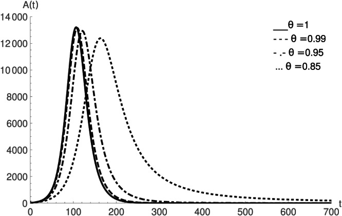
Nature of asymptomatic infectious population for different fractional order values when $\rho =1.2$

FIGURE 4.

Nature of infectious class for different fractional order values when $\rho =1.2$

FIGURE 5.

Nature of isolated infected class for different fractional order values when $\rho =1.2$

FIGURE 6.

Nature of recovered class for different fractional order values when $\rho =1.2$

FIGURE 7.

Nature of susceptible class for different values of parameter ρ when θ fixed at 1

FIGURE 8.

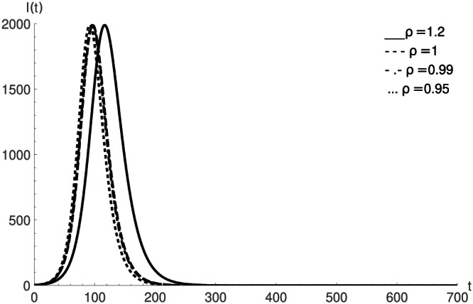
Nature of infectious class for different values of parameter ρ when θ fixed at 1

7. CONCLUSIONS

In this manuscript, we analysed a fractional coronavirus model to study the coronavirus outbreaks in India with a true data up to 30 April 2020. We have studied the proposed time non‐integer order model of coronavirus by the application of a modified version of Predictor‐Corrector scheme in the framework of new generalised form of Caputo non‐integer order derivative. The existence of unique solution for the given fractional order generalised Caputo system is also analysed by the results of fixed point theory. We use the definition of Chebyshev norm, Banach space, Schauders second fixed point theorem, Arzel's‐Ascoli theorem, uniform boundedness, equicontinuity and Weissingers fixed point theorem to perform the existence of unique solution. Our results are helpful to compare the model outputs more closer to the real data of India. All important plots are discussed to clarify the importance of the given solutions at various order values of θ at different values of parameter ρ . The mentioned method is recent and highly strong in analysing the solution to non‐classical dynamical models of physical, medical and biological views. The stability results of the projected method are also investigated. The given numerical approach exemplifies the applications of the newly proposed Caputo derivative to analyse the real word problems.

Kumar P, Erturk VS. A case study of Covid‐19 epidemic in India via new generalised Caputo type fractional derivatives. Math Meth Appl Sci. 2021;1–14. 10.1002/mma.7284

REFERENCES

- 1. Mission WCJ. Report of the WHO‐China Joint Mission on Coronavirus Disease 2019 (covid‐19). Geneva 2020; 2020.
- 2. Zhu N, Zhang D, Wang W, et al. A novel coronavirus from patients with pneumonia in China, 2019. New England J Med. 2020;382:727‐733. [DOI] [PMC free article] [PubMed] [Google Scholar]
- 3. Bastos SB, Cajueiro DO. Modeling and forecasting the early evolution of the Covid‐19 pandemic in Brazil. arXiv preprint arXiv:200314288; 2020. [DOI] [PMC free article] [PubMed]
- 4. Erturk VS, Kumar P. Solution of a Covid‐19 model via new generalized Caputo‐type fractional derivatives. Chaos, Solitons Fractals. 2020;139:110280. [DOI] [PMC free article] [PubMed] [Google Scholar]
- 5. Nadim SS, Ghosh I, Chattopadhyay J. Short‐term predictions and prevention strategies for Covid‐2019: A model based study. arXiv preprint arXiv:200308150; 2020. [DOI] [PMC free article] [PubMed]
- 6. Nabi KN, Abboubakar H, Kumar P. Forecasting of Covid‐19 pandemic: From integer derivatives to fractional derivatives. Chaos, Solitons Fractals. 2020;141:110283. [DOI] [PMC free article] [PubMed] [Google Scholar]
- 7. Kumar P, Suat Erturk V. The analysis of a time delay fractional Covid‐19 model via Caputo type fractional derivative. Math Methods Appl Sci. [DOI] [PMC free article] [PubMed] [Google Scholar]
- 8. Gao W, Veeresha P, Baskonus HM, Prakasha DG, Kumar P. A new study of unreported cases of 2019‐nCov epidemic outbreaks. Chaos, Solitons Fractals. 2020;138:109929. [DOI] [PMC free article] [PubMed] [Google Scholar]
- 9. Rashid S, Baleanu D, Chu Y‐M. Some new extensions for fractional integral operator having exponential in the kernel and their applications in physical systems. Open Phys. 2020;18(1):478‐491. [Google Scholar]
- 10. Rashid S, İşcan I, Baleanu D, Chu Y‐M. Generation of new fractional inequalities via n polynomials s‐type convexity with applications. Adv Differ Equa. 2020;2020(1):1‐20. [Google Scholar]
- 11. Khan ZA, Rashid S, Ashraf R, Baleanu D, Chu Y‐M. Generalized trapezium‐type inequalities in the settings of fractal sets for functions having generalized convexity property. Adv Differ Equa. 2020;2020(1):1‐24. [Google Scholar]
- 12. Nikan O, Jafari H, Golbabai A. Numerical analysis of the fractional evolution model for heat flow in materials with memory. Alexand Eng J. 2020;59(4):2627‐2637. [Google Scholar]
- 13. Rashid S, Kalsoom H, Hammouch Z, Ashraf R, Baleanu D, Chu Y‐M. New multi‐parametrized estimates having pth‐order differentiability in fractional calculus for predominating‐convex functions in Hilbert space. Symmetry. 2020;12(2):222. [Google Scholar]
- 14. Rashid S, Jarad F, Noor MA, Kalsoom H, Chu Y‐M. Inequalities by means of generalized proportional fractional integral operators with respect to another function. Mathematics. 2019;7(12):1225. [Google Scholar]
- 15. Kilbas A. Theory and Applications of Fractional Differential Equations. New York: Elsevier. [Google Scholar]
- 16. Miller KS, Ross B. An Introduction to the Fractional Calculus and Fractional Differential Equations. New York: Wiley; 1993. [Google Scholar]
- 17. Oldham K, Spanier J. The Fractional Calculus Theory and Applications of Differentiation and Integration to Arbitrary Order. New York: Elsevier; 1974. [Google Scholar]
- 18. Podlubny I. Fractional Differential Equations: An Introduction to Fractional Derivatives, Fractional Differential Equations, to Methods of Their Solution and Some of Their Applications. New York: Elsevier; 1998. [Google Scholar]
- 19. Rudolf H. Applications of Fractional Calculus in Physics. Singapore: World Scientific; 2000. [Google Scholar]
- 20. Odibat Z, Baleanu D. Numerical simulation of initial value problems with generalized Caputo‐type fractional derivatives. Appl Numer Math. 2020;156:94‐105. [Google Scholar]
- 21. Baleanu D, Wu G‐C, Zeng S‐D. Chaos analysis and asymptotic stability of generalized Caputo fractional differential equations. Chaos, Solitons Fractals. 2017;102:99‐105. [Google Scholar]
- 22. Qureshi S, Yusuf A. Modeling chickenpox disease with fractional derivatives: From Caputo to Atangana‐Baleanu. Chaos, Solitons Fractals. 2019;122:111‐118. [Google Scholar]
- 23. Kumar P, Rangaig NA, Abboubakar H, Kumar S. A malaria model with Caputo‐Fabrizio and Atangana‐Baleanu derivatives. Int J Model Simul Scie Comput. 2020. [Google Scholar]
- 24. Kumar P, Erturk VS. Environmental persistence influences infection dynamics for a butterfly pathogen via new generalised Caputo type fractional derivative. Chaos, Solitons Fractals. 2021;144:110672. [Google Scholar]
- 25. Muhammad Altaf K, Atangana A. Dynamics of Ebola disease in the framework of different fractional derivatives. Entropy. 2019;21(3):303. [DOI] [PMC free article] [PubMed] [Google Scholar]
- 26. Rivero M, Trujillo JJ, Vázquez L, Velasco MP. Fractional dynamics of populations. Appl Math Comput. 2011;218(3):1089‐1095. [Google Scholar]
- 27. Babaei A, Jafari H, Ahmadi M. A fractional order HIV/AIDS model based on the effect of screening of unaware infectives. Math Methods Appl Sci. 2019;42(7):2334‐2343. [Google Scholar]
- 28. Babaei A, Jafari H, Liya A. Mathematical models of HIV/AIDS and drug addiction in prisons. Eur Phys J Plus. 2020;135(5):395. [Google Scholar]
- 29. Ganji R, Jafari H. A new approach for solving nonlinear Volterra integro‐differential equations with Mittag‐Leffler kernel. Proc Inst Math Mech Natl Acad Sci Azerb. 2020;46:144‐158. [Google Scholar]
- 30. Sadeghi S, Jafari H, Nemati S. Operational matrix for Atangana‐Baleanu derivative based on Genocchi polynomials for solving FDES. Chaos, Solitons Fract. 2020;135:109736. [Google Scholar]
- 31. Ganji RM, Jafari H, Baleanu D. A new approach for solving multi variable orders differential equations with Mittag–Leffler kernel. Chaos, Solitons Fractals. 2020;130:109405. [Google Scholar]
- 32. Baleanu D, Mousalou A, Rezapour S. On the existence of solutions for some infinite coefficient‐symmetric Caputo‐Fabrizio fractional integro‐differential equations. Bound Value Probl. 2017;2017(1):1‐9. [Google Scholar]
- 33. Katugampola UN. Existence and uniqueness results for a class of generalized fractional differential equations. arXiv preprint arXiv:14115229; 2014.
- 34. Li C, Zeng F. The finite difference methods for fractional ordinary differential equations. Numer Funct Anal Optim. 2013;34(2):149‐179. [Google Scholar]
- 35. Sarkar K, Khajanchi S, Nieto JJ. Modeling and forecasting the Covid‐19 pandemic in India. Chaos, Solitons Fractals. 2020;139:110049. [DOI] [PMC free article] [PubMed] [Google Scholar]