Abstract
The objective of this research is to develop a convolutional neural network model ‘COVID‐Screen‐Net’ for multi‐class classification of chest X‐ray images into three classes viz. COVID‐19, bacterial pneumonia, and normal. The model performs the automatic feature extraction from X‐ray images and accurately identifies the features responsible for distinguishing the X‐ray images of different classes. It plots these features on the GradCam. The authors optimized the number of convolution and activation layers according to the size of the dataset. They also fine‐tuned the hyperparameters to minimize the computation time and to enhance the efficiency of the model. The performance of the model has been evaluated on the anonymous chest X‐ray images collected from hospitals and the dataset available on the web. The model attains an average accuracy of 97.71% and a maximum recall of 100%. The comparative analysis shows that the ‘COVID‐Screen‐Net’ outperforms the existing systems for screening of COVID‐19. The effectiveness of the model is validated by the radiology experts on the real‐time dataset. Therefore, it may prove a useful tool for quick and low‐cost mass screening of patients of COVID‐19. This tool may reduce the burden on health experts in the present situation of the Global Pandemic. The copyright of this tool is registered in the names of authors under the laws of Intellectual Property Rights in India with the registration number ‘SW‐13625/2020’.
Keywords: CNN model, Corona, COVID‐19, deep learning, global pandemic, X‐ray

1. INTRODUCTION
The world is facing a serious health emergency due to the outbreak of ‘COVID‐19’ since January 2020. This communicable disease is caused by the human coronavirus “SARS‐CoV‐2”. The first infection notified in Wuhan, China in December 2019, spread out in 220 countries and lead to a global pandemic. World Health Organization (WHO) reported the infection in 77 807 440 people. The virus caused the death of 1 711 286 people across the globe until December 22, 2020. 1 The discussion given in Reference 2 provides insights into the spreading trends of COVID‐19. It also provides details about the AI‐based tools available for presenting the data analytics and predicting the COVID‐19 outbreak. Timely and accurate diagnosis is important to control this outbreak. The teams of doctors, scientists, research communities, and diagnostic kit manufacturers are working hard to provide low‐cost and quick methods to diagnose this disease. They developed two types of immunodiagnostic Rapid Diagnostic Tests (RDT) tests viz. “RDT based on antigen detection”, and “RDT based on host antibody detection”. 3 The accuracy of ‘RDT based on antigen detection’ is dependent on the concentration of viruses in the sample collected from the respiratory tract. On the other hand, the accuracy of ‘RDT based on host antibody’ is dependent on the number of antibodies present in the blood of the patient. The antibody formation is highly decided by the age, nutrition, and prior health conditions of the person. 4 These tests are not reliable due to low accuracy and dependency on other factors such as age, nutrition, health history, etc. Therefore, the WHO does not recommend the above‐stated tests for diagnostic purposes. But, the usage of these tests for research is encouraged. 5
WHO recommended molecular tests such as Polymerase Chain Reaction (PCR) as a confirmatory and laboratory test for COVID‐19. 6 But, the test is restricted to the limited number of Government and Private Laboratories. Moreover, the effectiveness of this test is dependent on the collection, packaging, and shipment of the samples. Its sensitivity is reported as 60%–70%. 7
The low accuracy of the PCR test motivates researchers and health experts to introduce more ways of diagnosis. The radiological examination has been a reliable diagnosing technique for infectious diseases such as bacterial pneumonia, viral pneumonia, and tuberculosis, etc. for many decades. The authors in Reference 8 claimed that the abnormality in the lungs is captured in the CXR. The changes in the shape, size, textures, and reflection symmetry between the lungs are examined to diagnose the abnormality or disease.
A discussion with a senior radiology expert clarified that there are remarkable differences in chest X‐ray images of non‐infected, patients of COVID‐19, and patients infected with bacterial pneumonia. He added that the typical bacterial pneumonia causes the opacities or pleural effusion to a confined region. Also, there is a regular pattern of opacities in X‐ray images of a person infected with bacterial pneumonia. The rate of spreading of bacterial pneumonia is slow. Therefore, the X‐ray images captured after every 2 or 3 days will show a minor variation in opacities. On the other hand, the irregular pattern of white patches or opacities is observed throughout the lungs in patients of COVID‐19. The opacities are bilateral and pleural effusion is observed in all the lobes of the lungs. The opacities are more common near hila. Also, the rate of spreading is very fast. The causing agent of COVID‐19 infects both the lungs completely within a short period of 2–3 days. The infection shows its large impact on both the lungs after 2–3 days. The authors in References 9, 10, 11 also claimed that the chest X‐ray images of confirmed patients of COVID‐19 show multi‐lobar opacities in the lungs. These opacities are ground glass and mixed attenuation.
The above discussion shows that the X‐ray images can be a useful modality for the screening of ‘COVID‐19’ due to remarkable differences captured for infected and healthy lungs. But, manual reading of X‐ray images is a time‐consuming task. It is difficult for health experts to guarantee a quick response in the present situation of the global pandemic. Therefore, it is mandatory to search for an alternative method of screening. The Deep Learning (DL) techniques automated the process of feature extraction and feature selection. 12 There is a provision to fine‐tune the features for obtaining the desired outcome. These techniques allow parallel computations and also learn about the variations in the datasets. Thus, DL techniques are effective in handling the huge and variegated datasets. 13 Convolutional Neural Networks (CNNs), a class of DL networks are useful in the automatic extraction of the relevant features from images and feature mapping. 13 Their fast computations, the ability of object detection, continuous learning, and precise classification are the motivations for the authors to employ CNN models in mass screening of COVID‐19 from chest X‐ray images. The basic architecture of the CNN model is shown in Figure 1.
FIGURE 1.

Basic architecture of CNN model [Color figure can be viewed at wileyonlinelibrary.com]
The CNN architecture comprises of following layers to perform different operations.
-
i
Convolution Layer: This layer receives the input image as a matrix of digits. It includes another matrix “filter” or “kernel”. The filter strides over an input image to extract features of the image without destructing the spatial relationship between the pixels. The convolution operation calculates the dot product of the input image and its filter. 14 The operation gives a feature map as shown in Figure 2C. Different filters generate different feature maps, so the convolution layer acts as a feature detector. Exemplified as the value of the first cell of the feature map is calculated as the dot product of the input image and filter striding over it as given below.
FIGURE 2.
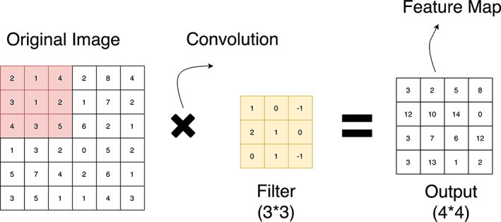
Convolution operation [Color figure can be viewed at wileyonlinelibrary.com]
((2*1) + (1*0) (+4*(−1)) + (3*2) + (1*1) + (2*0) + (4*0) + (3*1) + (5*(−1))).
The input image and the filter considered for calculation of the value of the first cell of the feature map are shown with the yellow boundary in Figure 2A, and Figure 2B, respectively. The value obtained is shown within the yellow boundary in Figure 2C. The filter strides repeatedly over the input matrix to obtain all the values of the feature map. The striding of filter over the input matrix with a stride of ‘1’ is shown in Figure 3.
-
ii
Pooling Layer: A pooling layer is a form of a non‐linear function. It is applied to a convoluted image to create a summary of the important features available in an image. The pooling layer reduces the number of parameters and computations on CNN. It reduces the resolution of a feature map but it does not lose its vital information. 14 In max pooling, the maximum value is picked from the feature map to determine the important features as shown in Figure 4. Selecting a subset of features finds fewer false patterns. Thus, this layer helps in controlling the problem of over‐fitting.
-
iii
Fully Connected Layer: This layer follows many convolutional layers and pooling layers. It represents a feature vector for an input image. It contains connections to all activations in a previous layer. This layer helps a network to learn the non‐linear combinations of features for classification. 14
FIGURE 3.
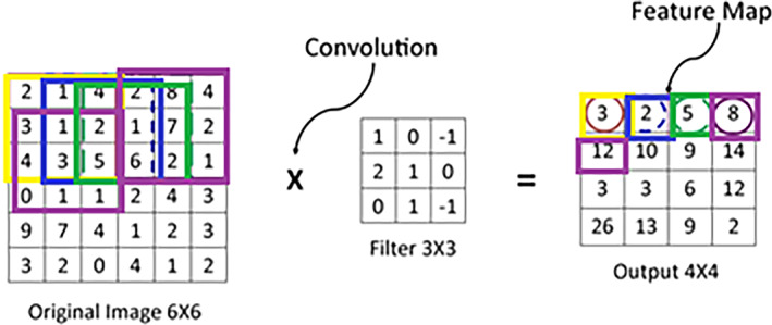
Striding of filter over an input image [Color figure can be viewed at wileyonlinelibrary.com]
FIGURE 4.
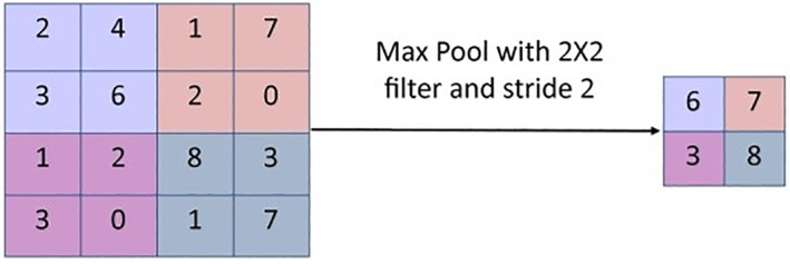
Max pooling operation [Color figure can be viewed at wileyonlinelibrary.com]
The applications of CNN in medical image analysis and classification attracted the researchers 11 , 15 , 16 , 17 , 18 , 19 to provide technological assistants to medical practitioners for dealing with the global pandemic of COVID‐19. The researchers in Reference 15 proposed the deep learning model “COVID‐Net” for the diagnosis of COVID‐19. The model reports the accuracy of 83.25% on X‐ray images of patients of COVID‐19 and bacterial pneumonia. The researchers in Reference 16 proposed the model “COVIDX‐Net” for the classification of non‐infected and patients of ‘COVID‐19’. It reports the highest accuracy of 90% that is an improvement of 6.75% over the model proposed in Reference 15.
The above‐stated models face challenges such as overfitting, high computation complexity, and low accuracy for multi‐class classification. To minimize these challenges, the authors in Reference 17 proposed a light‐weight CNN‐tailored shallow architecture for the detection of COVID‐19 using CXRs. They experimented with 130 CXR of positive cases of COVID‐19 and 51 CXRs of Non‐COVID cases. Their model achieved the highest sensitivity and accuracy of 94.43% and 96.92%, respectively. The authors claimed that their model outperformed the DL tools, such as MobileNet and VGG‐16. Also, their model is computationally efficient due to less number of parameters. A combination of the CNN model and SVM classifier proposed in Reference 18 reports the accuracy of 95.38% for the detection of COVID‐19. The authors in Reference 19 claimed that applying ResNet‐50 on X‐ray images gives an accuracy of 98%. But they tested their model only on the dataset of 50 images. The researchers in Reference 11 proposed the CNN model “DarkCovidNet” for the diagnosis of COVID‐19. They developed the model with 17 convolution layers and trained their model with publicly available datasets. 20 , 21 The model reported the highest accuracy of 98.08% for the binary classification and 87.02% for the multiclass classification. However, the proposed models reported good accuracy in classification. But, there is a scope for improving the accuracy of multiclass classification.
In this manuscript, the authors propose the convolutional neural network model “COVID‐Screen‐Net” for the screening of ‘COVID‐19’ using the chest X‐ray images. The design of the model is customized in such a way that it can accurately classify the X‐ray images of COVID‐19 even though trained with a small dataset. The model employs the GradCam for visualizing the most prominent features involved in the prediction of the infected regions of the lungs. This may prove useful to clinicians to validate the results of the model. The major contributions of this manuscript are as follows.
To collect the anonymous dataset of chest X‐rays from hospitals and different sources available online.
The cleaning and pre‐processing of the dataset.
The validation of the labeled dataset by the radiology experts.
To utilize the potential of CNN in object detection and pattern matching for detection of COVID‐19 in chest X‐rays.
To develop a CNN model for mass screening of non‐infected persons (normal), patients infected with COVID‐19 and bacterial pneumonia into three classes viz. normal, COVID‐19, and bacterial pneumonia.
To optimize the hyperparameters of the CNN model according to the training dataset.
To provide a tool for the mass screening of COVID‐19 with higher sensitivity and specificity than the tools and techniques proposed in the literature.
To present the visualization of the most prominent features involved in distinguishing the X‐ray images into three classes viz. normal, COVID‐19, and bacterial pneumonia.
2. MATERIALS AND METHODS
In this section, the authors demonstrate the data set used, detailed architecture, and working of the proposed CNN model “COVID‐Screen‐Net”.
2.1. Dataset
The authors used the dataset of 3000 X‐ray images, publicly available at. 20 , 21 The dataset contains 975 images of non‐infected persons, 950 images of patients of ‘COVID‐19’, and 950 images of patients of “Bacterial Pneumonia”. Figure 5A–C shows the sample X‐ray images of ‘COVID‐19’, normal and bacterial pneumonia respectively.
FIGURE 5.
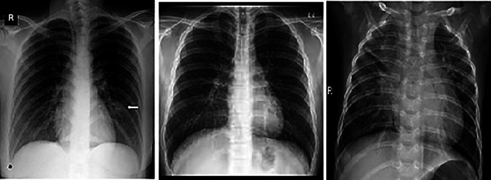
(A) ‘COVID‐19’, (B) normal, and (C) bacterial pneumonia
The authors divided the dataset into training, testing, and validation datasets. The testing set comprises 80% of the total X‐ray images whereas the testing set contains 20% of the total dataset. The validation set comprises 10% of images randomly chosen from the training dataset. The authors also divided the dataset into 47 batches. Each batch contains 64 images. The model receives 38 batches in each epoch during the training and 19 batches during the testing. The authors conducted a set of experiments to select the appropriate batch size. This chosen batch size allows the model to gradually learn the features of the dataset. It minimizes the chances of making the model familiar with the whole dataset at the beginning of the training. Thus, it reduces the problem of generalization. 22
2.2. The architecture of “COVID‐Screen‐Net”
The model ‘COVID‐Screen‐Net’ is an effective application of 2‐Dimensional (2‐D) Convolutional Neural Networks (CNNs). It comprises five convolution layers. Each convolution layer is alternatively followed by a global max‐pooling layer. The first convolution layer uses 32 filters and a kernel size of 3 × 3. It employs the ReLU activation function. 13 The next four convolution layers consist of 64 filters and a kernel size of 2 × 2. The feature map obtained on applying the five convolutions and max‐pooling operations is given as an input to the flattened layer. The flattened layer is further connected to the fully connected dense layer which employs the “softmax” activation function. The overall architecture of the model is shown in Figure 6.
FIGURE 6.

Architecture of “COVID‐Screen‐Net” [Color figure can be viewed at wileyonlinelibrary.com]
2.3. Working of “COVID‐Screen‐Net”
The model ‘COVID‐Screen‐Net’ performs a sequence of operations for the screening of COVID‐19, bacterial pneumonia, and normal as presented in Algorithm 1.
Pre‐processing: The model receives X‐ray images of dimensions 256 × 256 × 32 as an input. It applies the resize and augmentation techniques for the pre‐processing of the input images. The authors applied the techniques for changing the contrast and brightness of X‐ray images. Therefore, two images corresponding to an original image are obtained. These augmentation techniques are useful for increasing the size of the dataset.
Feature extraction: The model uses pre‐processed X‐ray images for feature extraction. It extracts the features and creates the feature maps using multiple convolutions and pooling operations. On a sample image of size 6 × 6, Figures 2 and 3, demonstrate the convolution and pooling operations respectively.
Visualization: The authors plotted the feature map obtained at the last activation layer. They used the GradCam to plot the feature map. The plotting at each convolution and activation layer gave an idea of how the model extracts all possible features in the initial layers and ignores the less prominent features in later layers.
Classification: The pre‐processed images are given as input to the first convolution layer which contains a set of 32 filters, each of kernel size 3 × 3. This layer employs the ReLU activation function (f(x)). 13 It is a non‐saturating activation function as given in Equation (1). It is applied to every pixel. It replaces negative values with zero. Thus, it eliminates negative values from a feature map. This function brings the non‐linearity in the output of neurons of the model. Hence, it improves the ability to learn the complicated and complex forms of non‐linear data. As claimed in Reference 13, ReLU is preferred over other activation functions such as sigmoid and tanh as it does not activate all neurons at the same time. This solves the problem of vanishing gradients for training deep learning models and improves the performance of the model.
| (1) |
Screening of ‘COVID‐19’.
Input: X‐ray images of the chest.
Output: Three classes: ‘COVID‐19’, normal and bacterial pneumonia.
Apply pre‐processing: resize and augmentation on input X‐ray images.
Pass the image into the Convolution layer to create the feature map.
Input the feature map to the Global Max Pooling layer for extracting the feature with maximum value.
Repeat steps 2 and 3 for n = 1 to 5.
Apply flattening on the output obtained from the last global max‐pooling layer to get the 1‐D array of features.
Pass the 1‐D array of features obtained in step 4 to the Dropout layer for reducing the number of neurons.
Establish the connections of neurons selected by the dropout layer to the fully connected dense layer.
Apply the “softmax” activation function.
Draw activation maps to highlight the features involved in actual decision making.
Obtain outputs into three classes: COVID‐19, normal and bacterial pneumonia as outputs.
The output of the first convolution layer is given to the first global max‐pooling layer. This layer extracts the features with the maximum value, from each feature map. It also makes the model learn even when a small change in data is performed. Therefore, it is useful in improving the adaptability of the model. Now, four convolutions and pooling operations are applied alternatively using the convolution layers and global max‐pooling layers. These operations reduce the dimensions of an input image and give an output of dimensions 8 × 8 × 64. The obtained output is given to the flattening layer which converts the multi‐dimensional feature map to a 1‐Dimensional (1‐D) array of size 4096. The 1‐D array is important to create one to one connection of the extracted features with the fully connected dense layer. Now, the dropout function is applied to reduce the number of neurons to 256. The change in the shape of output and trainable parameters of the “COVID‐Screen‐Net” are shown in Table 1. These 256 neurons establish the connections with the next fully connected dense layer. The fully connected dense layer employs the “softmax” activation function 13 for predicting the probability distribution of outputs into multiple classes namely “COVID‐19”, normal, and ‘bacterial Pneumonia. Figure 7 demonstrates the black box working of the ‘COVID‐Screen‐Net’.
TABLE 1.
Shape of output and number of trainable parameters of ‘COVID‐Screen‐Net
| Name of layer | Shape of output | Number of trainable parameters |
|---|---|---|
| conv2d_11 (Conv2D) | (None, 256, 256, 32) | 896 |
| activation_13 (Activation) | (None, 256, 256, 32) | 0 |
| max_pooling2d_11 (MaxPooling) | (None, 128, 128, 32) | 0 |
| conv2d_12 (Conv2D) | (None, 128, 128, 64) | 8256 |
| activation_14 (Activation) | (None, 128, 128, 64) | 0 |
| max_pooling2d_12 (MaxPooling) | (None, 64, 64, 64) | 0 |
| conv2d_13 (Conv2D) | (None, 64, 64, 64) | 16 448 |
| activation_15 (Activation) | (None, 64, 64, 64) | 0 |
| max_pooling2d_13 (MaxPooling) | (None, 32, 32, 64) | 0 |
| conv2d_14 (Conv2D) | (None, 32, 32, 64) | 16 448 |
| activation_16 (Activation) | (None, 32, 32, 64) | 0 |
| max_pooling2d_14 (MaxPooling) | (None, 16, 16, 64) | 0 |
| conv2d_15 (Conv2D) | (None, 16, 16, 64) | 16 448 |
| activation_17 (Activation) | (None, 16, 16, 64) | 0 |
| max_pooling2d_15 (MaxPooling) | (None, 8, 8, 64) | 0 |
| flatten_3 (Flatten) | (None, 4096) | 0 |
| dense_5 (Dense) | (None, 256) | 1 048 832 |
| activation_18 (Activation) | (None, 256) | 0 |
| dropout_3 (Dropout) | (None, 256) | 0 |
FIGURE 7.

Black Box working of the ‘COVID‐Screen‐Net’ [Color figure can be viewed at wileyonlinelibrary.com]
3. EXPERIMENTS
The authors used the memory and processing resources available at Google Colab 23 for conducting the experiments. Google Colab is an online training platform freely available for storage and processing. It provides the facility of processing the data on Tesla K80 GPU and RAM capacity of 12 GB. It is efficient in the continuous execution of a model for 12 hr without any halt. The authors used the dataset in References 20, 21 for training the “COVID‐Screen‐Net”. They fine‐tuned the training parameters given in Section 3.1 to optimize the performance of the model.
3.1. Training parameters
The proposed model employs the RMSProp optimizer 13 at the dense layer. The model uses the following training parameters.
rho: This is the exponentially weighted average over the square of the gradients. It is the decay factor for the learning rate of the model. In this manuscript, the authors pre‐set the optimum value of ‘rho’ as 0.9. The value is determined by performing the set of experiments. Figure 8 demonstrates the impact of change in the value of ‘rho’, on the accuracy of the model. The increase in the value of ‘rho’ above 0.9 leads to a sharp decrease in the accuracy. On the contrary, the decrease in value of ‘rho’ below 0.9 shows a gradual increase or decrease in the accuracy. The variation in the accuracy, Area Under Curve(AUC), precision, recall, and F1 measure with the change in the value of ‘rho’ is shown in Table 2.
Decay rate: This is the learning rate of the model. The model reaches close to the local minimum at the end of the training. In this research, the authors set the decay rate as ‘0’. The value is determined after conducting a set of experiments. Figure 9 demonstrates the effect of the decay rate on accuracy. At the pre‐set value ‘0’, the model attains the optimum value of the decay rate as 0.0001. An increase in the decay rate sharply decreases the accuracy of the model. Table 3 shows the variation in the performance metrics namely accuracy, AUC, precision, recall, and F1 measure of the “COVID‐Screen‐Net” with the change in the value of decay rate.
Learning Rate: This hyper‐parameter determines the rate of learning of the machine‐learning model. It decides the number of steps the model requires to minimize the value of the loss function. Figure 10 demonstrates the effect of the learning rate on the accuracy of the “COVID‐Screen‐Net”. In this research, the authors set the value of the learning rate as 0.0004 based on the set of experiments. The impact of the learning rate on the performance of the model is shown in Table 4.
Epsilon: This parameter prevents the erroneous values of gradients such as divided by zero. In this manuscript, the authors used the default value of epsilon as 1e‐10.
FIGURE 8.
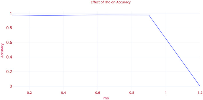
Effect of “rho” on the accuracy of ‘COVID‐Screen‐Net’ [Color figure can be viewed at wileyonlinelibrary.com]
TABLE 2.
Impact of ‘rho’ on performance of ‘COVID‐Screen‐Net’
| rho | Accuracy | AUC score | Precision | Recall | F1 score |
|---|---|---|---|---|---|
| 0.1 | 0.977193 | 0.983171 | 0.97724 | 0.977193 | 0.977132 |
| 0.3 | 0.97193 | 0.978834 | 0.972215 | 0.97193 | 0.972016 |
| 0.6 | 0.978947 | 0.984122 | 0.978991 | 0.978947 | 0.978951 |
| 0.9 | 0.977193 | 0.982703 | 0.977288 | 0.977193 | 0.977152 |
| 1.2 | 0 | 0.5 | 0 | 0 | 0 |
FIGURE 9.
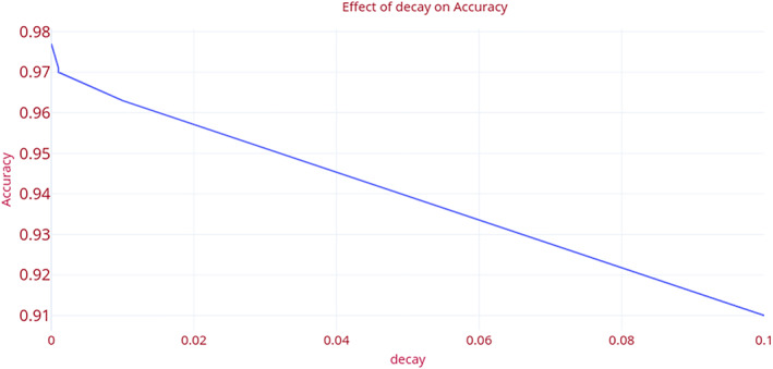
Effect of “decay rate” on the accuracy of ‘COVID‐Screen‐Net’ [Color figure can be viewed at wileyonlinelibrary.com]
TABLE 3.
Impact of decay on performance of ‘COVID‐Screen‐Net’
| Decay | Accuracy | AUC score | Precision | Recall | F1 score |
|---|---|---|---|---|---|
| 0 | 0.977193 | 0.982703 | 0.977288 | 0.977193 | 0.977152 |
| 1.00E‐05 | 0.97193 | 0.978544 | 0.972835 | 0.97193 | 0.972057 |
| 1.00E‐04 | 0.970175 | 0.977392 | 0.97074 | 0.970175 | 0.970299 |
| 1.00E‐03 | 0.970175 | 0.977247 | 0.970755 | 0.970175 | 0.970214 |
| 1.00E‐02 | 0.963158 | 0.972273 | 0.963365 | 0.963158 | 0.963205 |
| 1.00E‐01 | 0.910526 | 0.93835 | 0.928938 | 0.910526 | 0.918254 |
FIGURE 10.
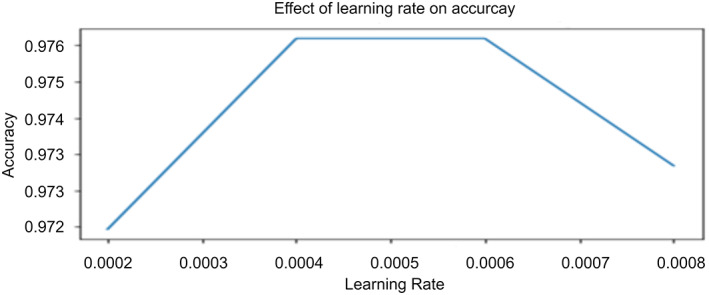
Impact of learning rate on accuracy of ‘COVID‐Screen‐Net’ [Color figure can be viewed at wileyonlinelibrary.com]
TABLE 4.
Impact of learning rate on performance of the ‘COVID‐Screen‐Net’
| Learning rate | Accuracy | AUC Score | Precision | Recall | F1 score |
|---|---|---|---|---|---|
| 0.00004 | 0.961404 | 0.971041 | 0.961547 | 0.961404 | 0.961436 |
| 0.0008 | 0.973684 | 0.979819 | 0.974499 | 0.973684 | 0.973728 |
| 0.0006 | 0.977193 | 0.98321 | 0.977268 | 0.977193 | 0.977137 |
| 0.0004 | 0.977193 | 0.982703 | 0.977288 | 0.977193 | 0.977152 |
| 0.004 | 0.975439 | 0.981681 | 0.975664 | 0.975439 | 0.975379 |
| 0.04 | 0 | 0.5 | 0 | 0 | 0 |
3.2. Results
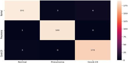
The authors assigned class labels 0, 1, and 2 to the normal, bacterial pneumonia, and “COVID‐19” respectively. Table 5 shows the confusion matrix of 570 images used in the testing dataset. The authors evaluated the performance of the “COVID‐Screen‐Net” using the following evaluation metrics.
-
i
Sensitivity(S): This is the percentage of the total number of correctly classified diseased instances in their labeled class. It is defined in Equation (2) for the class ‘COVID‐19’, and Equation (4) for the class ‘bacterial pneumonia’. The “COVID‐Screen‐Net” achieves the highest sensitivity of 98.34% for the ‘COVID‐19’ as calculated in Equation (3). It reports the highest sensitivity of 99.47% for bacterial pneumonia as calculated in Equation (5).
TABLE 5.
Confusion matrix of COVID‐Screen‐Net on test dataset [Color Table can be viewed at wileyonlinelibrary.com]
|
| (2) |
| (3) |
| (4) |
| (5) |
-
ii
Specificity (Sp): This is the percentage of the correctly classified instances to the normal class as defined in Equation (6). The “COVID‐Screen‐Net” achieves the specificity of 95.50% as calculated in Equation (7).
| (6) |
| (7) |
-
iii
Prevalence (P): This is the degree of contribution of a class in the complete dataset. Its definition is given in Equation (8). The dataset used for testing the models “COVID‐Screen‐Net”, “DarkCovid Net”, “VGG‐19”, and “ResNet‐50” reports the prevalence of 0.3175 for the COVID‐19, 0.3315 for bacterial pneumonia, and 0.3508 for the normal class as calculated in Equations (9), (10), and (11) respectively.
| (8) |
| (9) |
| (10) |
| (11) |
-
iv
Average Accuracy (Avg_Acc): This is the sum of products of prevalence with sensitivity and specificity as defined in Equation (12). The proposed model ‘COVID‐Screen‐Net’ reports the average accuracy of 99.71% on the test dataset as calculated in Equation (13).
| (12) |
| (13) |
The accuracy of the ‘COVID‐Screen‐Net’ randomly varies when it is executed from the 0th to the 120th epoch. Figure 11 demonstrates the trends of its accuracy until the model achieves its highest accuracy. It is clear from Figure 11 that the accuracy sharply increases in executing the model from 0th to 10th epochs. It achieves the maximum accuracy of 97.71% at the 50th epoch. On further training, the model gives a random increase and decrease inaccuracy. The trends of increase and decrease in the accuracy give the information that the model gradually learns about the dataset and the training parameters.
FIGURE 11.
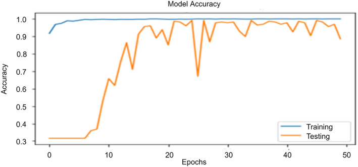
Trends of accuracy with change in number of epochs [Color figure can be viewed at wileyonlinelibrary.com]
The accuracy of the model is also dependent on the batch size. It achieves an accuracy of 94% when a batch size of 16 images is given as an input. On the contrary, the accuracy decreases and becomes 90.5% when the batch size is increased to 128 images. The maximum accuracy of 97.71% is achieved for the optimum batch size of 32 images.
-
v
Categorical cross‐entropy loss: It measures the degree of dissimilarity between the actual label distribution (y) and the predicted label distribution The definition of the categorical cross‐entropy loss ( is given in Equation (14). Here, i denotes the epoch number.
| (14) |
On performing the set of experiments, the authors recorded the values of loss as shown in Figure 12. There is a random increase and decrease in the values of the loss function when the number of epochs increases from 1 to 50. It reveals that the model is continuously learning the training parameters using the values of loss obtained in previous epochs. Repetitive learning is important for training the model and improving its efficacy. The model achieves the highest accuracy at the lowest value of the loss. It is clear from Figure 12, that the “COVID‐Screen‐Net” gives the minimum value of the loss at the 50th epoch. Therefore, it reports the maximum accuracy at this epoch. On further training, the model does not make a significant change in the value of the loss. It proves that the model is trained successfully and hence, can correctly predict the class of an input image.
-
vi
Area Under Curve (AUC): This is the area under the Receiver Operating Characteristic curve (ROC). ROC is the graphical representation of the number of correct predictions in a particular class against the number of wrong predictions made in that class. It directly determines the performance of the multi‐class model. The confusion matrix given in Table 5, shows the number of test images predicted correctly in their labeled classes. The high values of AUC under ROC 0.97 for the class label ‘0’ (normal), 0.99 for the class label “1” (bacterial pneumonia), and 0.98 (COVID‐19) for the class label “2” prove that the model is effective in making the correct predictions for each class. Figure 13 demonstrates the average ROC for all three classes.
-
vii
Precision: It is the ratio of the number of correct predictions in a particular class to that of the total number of correct predictions made in all the classes. The model “COVID‐Screen‐Net” achieves the maximum precision of 100% on the test dataset. The values of the precision of each class are shown in Figure 14. The high values of precision prove that the model is effective in extracting the relevant instances of each class label from the total number of extracted instances.
-
viii
Recall: It is the ratio of the number of correct predictions to a particular class to that of the total number of predictions made in that class. The model ‘COVID‐Screen‐Net’ gives the maximum recall of 100%. The values of recall for the class label ‘1’ and ‘2’ prove that the model extracts all the relevant instances from the given instances. Figure 14 shows the values of recall for each class.
-
ix
F1 Score: This is the harmonic mean of precision and recall. The proposed model gives an average F1 score of 99.6%. The high values of the F1 score prove, its efficacy in classifying the test images correctly into their actual classes viz. normal, ‘bacterial pneumonia’, and ‘COVID‐19’.
The performance of the model is recorded for a different number of epochs while training and testing for each class. It is observed that the model achieved the best performance at the 50th epoch. Figure 15 demonstrates the variation in the performance of the model with a change in the number of epochs.
FIGURE 12.
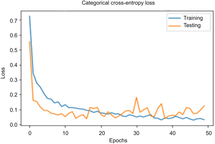
Trends of the value of loss with change in the number of epochs [Color figure can be viewed at wileyonlinelibrary.com]
FIGURE 13.
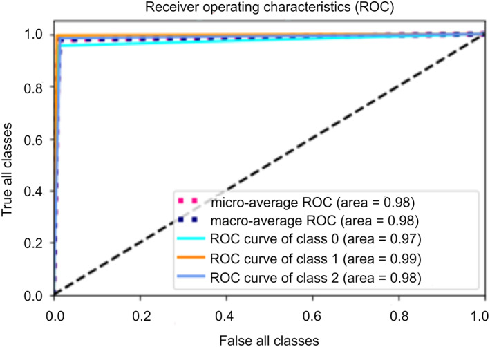
Average ROC for all the three classes [Color figure can be viewed at wileyonlinelibrary.com]
FIGURE 14.
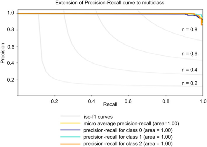
Performance of ‘COVID‐Screen‐Net’ for Normal, Bacterial Pneumonia, and COVID‐19 [Color figure can be viewed at wileyonlinelibrary.com]
FIGURE 15.
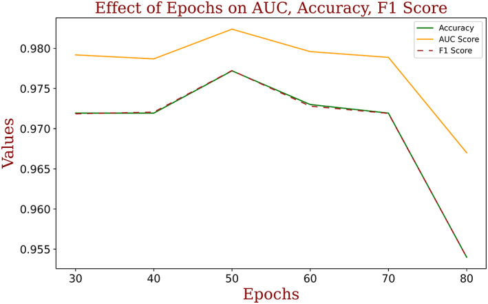
Performance of ‘COVID‐Screen‐Net’ with a change in the number of epochs [Color figure can be viewed at wileyonlinelibrary.com]
3.3. Comparative analysis
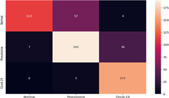
The authors executed the “DarkCovidNet”, “VGG‐19”, and “ResNet‐50” on the dataset in References 20, 21. They used the same dataset for training and testing of the proposed model “COVID‐Screen‐Net”. The Confusion matrices of “DarkCovidNet”, “VGG‐19”, and “ResNet‐50” are shown in Tables 6, 7, and 8 respectively. The “DarkCovidNet” reports a sensitivity of 96.87% for COVID‐19 and 81.54% for the bacterial pneumonia class. The model reports the specificity of 64.94% for the normal class. This model achieves the maximum average accuracy of 80.57% as calculated in Equation (15).
TABLE 6.
Confusion matrix of ‘DarkCovidNet’ on test dataset [Color Table can be viewed at wileyonlinelibrary.com]
|
TABLE 7.
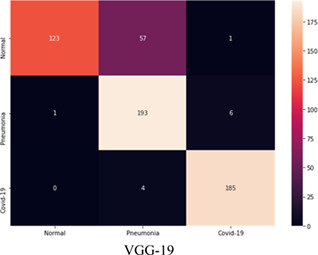
Confusion matrix of ‘VGG‐19’ on test dataset [Color Table can be viewed at wileyonlinelibrary.com]
|
TABLE 8.
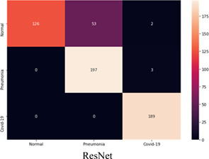
Confusion matrix of ‘ResNet50’ on test dataset [Color Table can be viewed at wileyonlinelibrary.com]
|
The model “VGG‐19” achieves the maximum sensitivity of 97.80% for the COVID‐19, 96.50% for the bacterial pneumonia class. The model achieves the specificity of 67.95% in the normal class. This model reports the highest average accuracy of 86.88%, as calculated in Equation (16).
The model “ResNet‐50” gave the maximum sensitivity of 100% for the COVID‐19 and 98.5% for the bacterial pneumonia Class. The model achieves a specificity of 68.85%. This model reports the maximum average accuracy of 88.55%, as calculated in Equation (17).
| (15) |
| (16) |
| (17) |
It is clear from the above discussion that the DarkCovidNet, VGG‐19, and ResNet‐50 are effective in classifying the samples of COVID‐19 and bacterial pneumonia class. But, these prove ineffective in the correct classification of the samples of the normal class. The high number of miss classification of the samples of ‘normal’ class to “COVID‐19” or ‘bacterial pneumonia’ classes degrade the reliability of these models. On the contrary, the proposed model “COVID‐Screen‐Net” correctly classifies the samples from each class. Thus, it achieves the highest average accuracy of 97.71% as calculated in Equation (12). Figure 16 demonstrates the comparison in the average accuracy of ‘COVID‐Screen‐Net’ with ‘DarkCovidNet’, ‘VGG‐19’, and ‘ResNet‐50’. The figure clearly shows that the model ‘COVID‐Screen‐Net’ outperforms the other three models.
FIGURE 16.
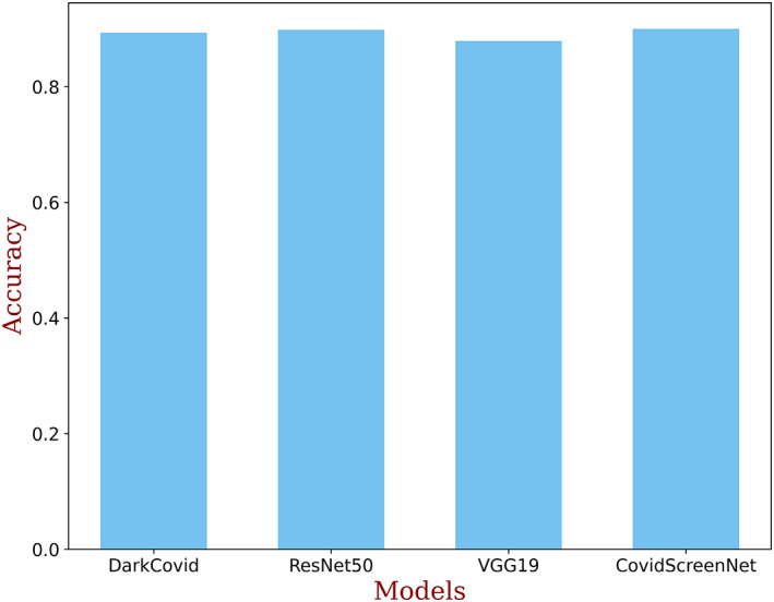
Comparison in the accuracy of DarkCovidNet, ResNet50, VGG‐19, and COVID‐Screen‐Net [Color figure can be viewed at wileyonlinelibrary.com]
The authors also made a comparison in the AUC score of ‘COVID‐Screen‐Net’ with ‘DarkCovidNet’, ‘VGG‐19’, and ‘ResNet‐50’. Figure 17 demonstrates the AUC score of these models. It is clear from Figure 17 that the ‘COVID‐Screen‐Net’ gives the maximum AUC score for the same dataset.
FIGURE 17.
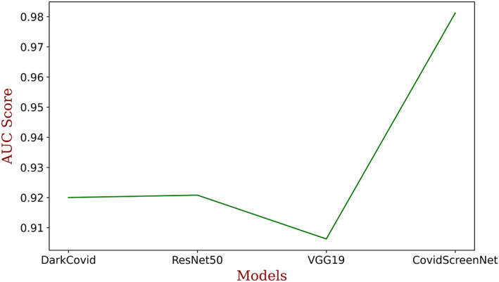
Comparison in AUC score of DarkCovidNet, ResNet50, VGG‐19, and COVID‐Screen‐Net [Color figure can be viewed at wileyonlinelibrary.com]
The execution time is an important factor to adopt the model for medical diagnosis. Therefore, the authors made a comparison in the execution time of the ‘COVID‐Screen‐Net’ with ‘DarkCovidNet’, ‘VGG‐19’, and ‘ResNet‐50’. The comparison in the execution time is shown in Figure 18. This figure shows that the ‘ResNet‐50’ takes the maximum time for computations. This is due to the more number of convolution and pooling layers in the model. The model ‘VGG‐19’ takes lesser time than ‘ResNet‐50’ but, it requires more time than ‘DarkCovidNet’ and ‘COVID‐Screen‐Net’. The Model ‘COVID‐Screen‐Net’ takes the minimum time for execution. This is due to the use of an optimum number of convolution and pooling layers in the network. The authors optimized the number of layers to overcome the problem of overfitting and to minimize the computation time. The authors applied the augmentation techniques to increase the size of the dataset. For training the model, they took an equivalent number of images in each class. Therefore, the model undergoes unbiased training. It resolved the problem of class imbalance and improves the average accuracy of the model.
FIGURE 18.
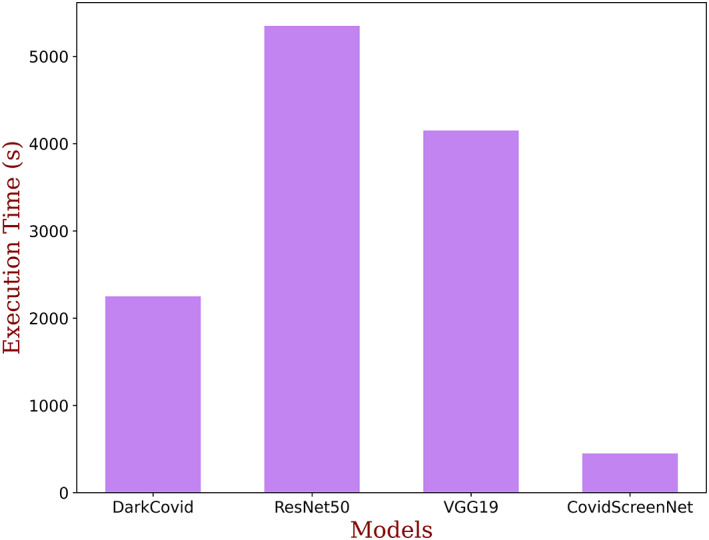
Comparison in execution time of DarkCovidNet, ResNet50, VGG‐19, and COVID‐Screen‐Net [Color figure can be viewed at wileyonlinelibrary.com]
4. DISCUSSION
Dr. Cohen collected and compiled the X‐ray images of the patients of “COVID‐19” confirmed by the RT‐PCR test. He made this data publicly available at the Github repository 20 for developing and evaluating the machine learning or deep learning models for the detection of ‘COVID‐19’. Similarly, Paul Mooney collected and compiled the X‐ray images from different sources for the confirmed cases the bacterial and viral pneumonia. He made these images available at the Kaggle repository. 21 But, the size of the dataset is small and is insufficient for the training of the deep learning models.
To provide a solution for the requirement of a huge training dataset, the authors in 24 discussed the importance of active learning in training for AI‐driven tools. In active learning, the model continuously receives the input data, detects the anomaly in the dataset if any, and consistently learns from it. The authors also focused that the potential of AI‐driven tools that can be utilized to diagnose the newly identified disease such as COVID‐19 by using the multitudinal and multimodel datasets for training. This is a time‐saving technique where the tools are trained using a dataset collected from one geographical region and the trained tools may prove useful in the diagnosis of a disease in a different region. For example, the COVID‐19 reported in China for the first time, and later on its cases are identified in other countries of the world. So, the dataset collected from China at an early stage can be used to train the model. This trained model with the feature of continuous learning may be useful in the screening of COVID‐19 across the world.
The researchers in Reference 11 proposed the deep learning model “DarkCovidNet” comprising 17‐convolution layers for the detection of COVID‐19. They evaluated their model on the dataset comprising 127 X‐ray images of COVID‐19 patients, 20 500 X‐ray images of no findings, and 500 X‐ray images of pneumonia. 21 They claimed an accuracy of 98.08% for the binary classification. But, the model reported an accuracy of 87.02% for the multi‐class classification. On executing the model on the dataset used for training and testing the “COVID‐Screen‐Net”, the model achieved the maximum average accuracy of 80.57%. This model employs a deep network of 17 layers for the small size of the dataset. Thus, it may lead to the problem of overfitting. Moreover, there is a huge difference in the size of datasets of COVID‐19 and the other two classes viz. No‐findings and Pneumonia. This may cause the problem of class imbalance.
The researchers in Reference 15 proposed the deep learning model “COVID‐Net” for the detection of COVID‐19. The model consists of 4‐convolution layers. They trained and evaluated their model on X‐ray images collected from References. 20 , 21 They used 68 X‐ray images of confirmed patients of ‘COVID‐19’, 1203 cases of healthy persons, 931 cases of bacterial pneumonia, and 660 cases of non‐COVID‐19 viral pneumonia. They reported an accuracy of 83.25% for the multi‐class classification. Similar to the model proposed in, 11 this model may undergo biased training due to the huge variation in the dataset size of different classes.
The researchers in Reference 16 proposed the deep learning framework “COVID‐NetX” based on the seven existing architectures. They compared the efficacy of seven deep learning models viz. VGG‐19, DenseNet201, Inception, ResNetV2, Xception, ResNetV2, and MobileNetV2 for detection of COVID‐19 using 50 X‐ray images of chest. They claimed that the VGG‐19 and DenseNet201 reported the highest accuracy of 90% on training and testing with 25 X‐ray images of COVID‐19 confirmed cases and 25 X‐ray images of non‐infected persons in Reference 18. They recommended the use of VGG‐19 and DenseNet201for detection of COVID‐19 using X‐ray images. The model ‘VGG‐19’ reported the average accuracy of 86.88% on the same dataset 20 , 21 as used for testing the “COVID‐Screen‐Net”.
The researchers in Reference 18 proposed the combination of the CNN model and SVM classifier. They reported an accuracy of 95.38% on training and testing their model using 25 X‐ray images of non‐infected persons and 25 X‐ray images of “COVID‐19” patients. 15
The authors in Reference 19 claimed that applying ResNet‐50 on X‐ray images reports an accuracy of 98% on binary classification into class labels namely “COVID‐19” and non‐infected. The evaluation of ResNet‐50 on the same dataset 20 , 21 as used for testing the ‘COVID‐Screen‐Net’ reported the average accuracy of 88.55%.
The authors in Reference 25 proposed the Truncated Inception Net model for classification of COVID‐19 positive from other non‐COVID cases and/or healthy CXRs. The model achieved an accuracy of 99.96%. The authors compared the performance of this model with COVID‐Net, 15 a combination of ResNet‐50 and SVM, 16 ResNet‐50, 18 and Inception Net V3. 19 Based on the comparison, they claimed that the Truncated Inception Net model outperformed these models.
The above discussion shows that the highest accuracy of multi‐class classification into normal, COVID‐19, and bacterial bneumonia is reported by the model proposed in Reference 19 is 88.55%. Employing deep networks for the small dataset and biased training are also limitations observed in this model. The deep learning model “COVID‐Screen‐Net” proposed in this manuscript performs the multi‐class classification and effective in the automatic screening of ‘COVID‐19’. The model reports an average accuracy of 97.71% on the testing dataset of 570 X‐ray images. To deal with the problem of biased training, the authors used an equal number of images for each class for training and testing the model. Moreover, the authors restricted the number of convolution layers to avoid the problem of overfitting on the small dataset. The model also presents the visualization of the features used by the model for automatic prediction of “COVID‐19” and “Bacterial Pneumonia”. The visualization in the GradCam may prove useful for clinicians in quick decision making. This model may prove an automatic and intelligent assistant for health experts. It can minimize the time and cost required for the screening of ‘COVID‐19’.
5. VALIDATION
The model is sent for validation to the radiology experts of RG Stone Urology & Laparoscopy Hospital. Dr. RK Sharma, Chief Radiologist, and Head Radio Diagnosis Division evaluated the efficacy of the model on the different types of chest radiographs of the patients and shared their feedback. The authors implemented the suggestions and improved the efficacy and reliability of the model by training the model with different types of chest radiographs such as low contrast and high contrast for each class namely ‘COVID‐19’, “bacterial pneumonia”, and normal. They validated the sensitivity and reliability of the model by testing the model on a real‐time dataset. The approval and recommendation are given as supplementary material.
6. CONCLUSION
The improvement in the efficacy of the health services has become the prime objective worldwide due to the “Global Pandemic” caused by the ‘COVID‐19’. The cost‐effective and timely diagnosis of the disease is important to reduce its outbreak. The deep learning model ‘COVID‐Screen‐Net’ can provide a technological solution for the screening of ‘COVID‐19’ using the X‐ray images of the chest. The model distinguishes the X‐ray images of normal, ‘bacterial pneumonia’, and ‘COVID‐19’. It reports the average accuracy of 97.71% on the test dataset of 570 X‐ray images publicly in References 20, 21
X‐ray imaging requires low cost and widely available. It also minimizes direct contact with the patient. Moreover, it avoids the risk of sample damage as observed in tests based on blood samples and swabs taken from the throat. The model can be employed at remote locations where the medical experts and lab facilities are not available. The radiographers can capture the X‐rays in contactless mode. They can use the model to classify normal and abnormal cases. The abnormal cases can be recommended for further medical tests and counseling on a priority basis. Therefore, this model may prove a useful assistant for medical practitioners in the quick screening of ‘COVID‐19’. This model can also be customized for the screening of ‘COVID‐19’ using CT scan images. Its applicability can be enhanced to classify the more number of diseases using chest radiographs.
A model is an effective tool for the classification of chest radiographs. But, its performance may degrade for the poor‐quality radiographs. The performance of the model may below in case the chest radiographs do not show any infection.
DATA AVAILABILITY
The data that support the findings of this study are openly available in ["Kaggle" and "Github"] at https://github.com/ieee8023/covid-chestxray-dataset, https://github.com/ieee8023/covid-chestxray-dataset [21–22]. The anonymous data collected from hospitals will be made available at "Github" repository at the publication stage of the article. The collected data will be made available with the consent from the health experts.
ACKNOWLEDGMENTS
We would like to thank Dr. Avinash, Dr. Deepak Buddhi, and Dr. Ravi Kumar, experts in the department of radiology at RG hospital Delhi for their valuable inputs. Their remarks and suggestions helped us to improve the robustness, average accuracy, and reliability of the model.
Dhaka VS, Rani G, Oza MG, Sharma T, Misra A. A deep learning model for mass screening of COVID‐19. Int J Imaging Syst Technol. 2021;31:483–498. 10.1002/ima.22544
REFERENCES
- 1. World Health Organisation . Naming the coronavirus disease (COVID‐19) and the virus that causes it. https://www.who.int/emergencies/diseases/novel-coronavirus-2019/technical-guidance/naming-the-coronavirus-disease-(COVID-2019)-and-the-virus-that-causes-it; 2020. Accessed April 8, 2020.
- 2. Joshi A, Dey N, Santosh KC. Intelligent systems and methods to combat Covid‐19, SpringerBriefs in Computational Intelligence; 2020, Springer Singapore, ISBN 978‐981‐15‐6572‐4, 10.1007/978-981-15-6572-4. [DOI]
- 3. World Health Organisation . Advice on the use of point‐of‐care immunodiagnostic tests for COVID‐19. https://www.who.int/news-room/commentaries/detail/advice-on-the-use-of-point-of-care-immunodiagnostic-tests-for-covid-19; 2020. Accessed May 10, 2020.
- 4. World Health Organisation . Advice on the use of point‐of‐care immunodiagnostic tests for COVID‐19. https://www.who.int/news-room/commentaries/detail/advice-on-the-use-of-point-of-care-immunodiagnostic-tests-for-covid-19. Accessed May 3, 2020.
- 5. Indian Council of Medical Research Department of Health Research . Additional_guidance_on_TrueNat_based_COVID19. https://icmr.nic.in/sites/default/files/upload_documents/Additional_guidance_on_TrueNat_based_COVID19_testing.pdf. Accessed April 27, 2020.
- 6. Indian Council of Medical Research Department of Health Research . Advisory on the feasibility of using pooled samples for molecular testing of COVID‐19. https://icmr.nic.in/sites/default/files/upload_documents/Advisory_on_feasibility_of_sample_pooling.pdf; 2020. Accessed on April 27, 2020.
- 7. Long C, Xu H, Shen Q, et al. Diagnosis of the coronavirus disease (COVID‐19): RRT‐PCR or CT? Eur J Radiol. 2020;126:108961. [DOI] [PMC free article] [PubMed] [Google Scholar]
- 8. Santosh KC, Antani S. Automated chest X‐ray screening: can lung region symmetry help detect pulmonary abnormalities? IEEE Trans Med Imaging. 2018;37(5):1168‐1177. 10.1109/TMI.2017.2775636. [DOI] [PubMed] [Google Scholar]
- 9. Kong W, Agarwal PP. Chest imaging appearance of COVID‐19 infection. Radiol: Cardiothoracic Imaging. 2020;2(1):e200028. [DOI] [PMC free article] [PubMed] [Google Scholar]
- 10. Kanne JP, Little BP, Chung JH, Elicker BM, Ketai LH. Essentials for radiologists on COVID‐19: an update—radiology scientific expert panel. Radiology. 2020;296:E113‐E114. 10.1148/radiol.2020200527. In press. [DOI] [PMC free article] [PubMed] [Google Scholar]
- 11. Ozturka T, Talob M, Yildirimc EA, Baloglud UB, Yildirime O, Rajendra Acharya U. f.Automated detection of COVID‐19 cases using deep neural networks with X‐ray images. Comput Biol Med. 2020;121:103792. 10.1016/j.compbiomed.2020.103792. [DOI] [PMC free article] [PubMed] [Google Scholar]
- 12. Yamashita R, Nishio M, Do RKG, Togashi K. Convolutional neural networks: an overview and application in radiology. Insights Imaging. 2018;9:611‐629. 10.1007/s13244-018-0639-9. [DOI] [PMC free article] [PubMed] [Google Scholar]
- 13. Krizhevsky A. ImageNet classification with deep convolutional neural networks, pp. 1–1432; 2010. 10.1201/9781420010749. [DOI]
- 14. Hijazi S, Kumar R, Rowen C. Using convolutional neural networks for image recognition. Cadence. 2015;55:1889‐1903. 10.2458/azu_js_rc.55.16783. [DOI] [Google Scholar]
- 15. Wang L, Wong A. COVID‐Net: a tailored deep convolutional neural network design for detection of COVID‐19 cases from chest radiography images. 2020. [DOI] [PMC free article] [PubMed]
- 16. Hemdan EE‐D, Shouman MA, Karar ME. COVIDX‐Net: a framework of deep learning classifiers to diagnose COVID‐19 in x‐ray images. arXiv:2003. 2020;11055. [Google Scholar]
- 17. Mukherjee H, Ghosh S, Dhar A, Obaidullah SM, Santosh KC, Roy K. Shallow convolutional neural network for COVID‐19 outbreak screening using chest x‐rays. TechRxiv. Preprint; 2020. 10.36227/techrxiv.12156522.v1 [DOI] [PMC free article] [PubMed]
- 18. Kumar P, Kumari S. Detection of coronavirus Disease (COVID‐19) based on Deep Features. Preprints; 2020.
- 19. Narin A, Kaya C, Pamuk Z. Automatic Detection of Coronavirus Disease (COVID‐19) Using X‐ray Images and Deep Convolutional Neural Networks. arXivPrepr. arXiv2003.10849; 2020. [DOI] [PMC free article] [PubMed]
- 20. Cohen . COVID chest x‐ray dataset. https://github.com/ieee8023/covid-chestxray-dataset; 2020. Accessed April 3, 2020).
- 21. Mooney . Kaggle chest x‐ray images (pneumonia) dataset. https://github.com/ieee8023/covid‐chestxray‐dataset; 2020. Accessed April 3, 2020.
- 22. Pradhan N, Dhaka VS, Rani G, Choudhary H. Transforming view of medical images using deep learning. Neural Comput Appl. 2020;32:1433‐3058. 10.1007/s00521-020-04857-z. [DOI] [Google Scholar]
- 23. Carneiro T, Da Nóbrega RVM, Nepomuceno T, et al. Performance analysis of Google Colaboratory is a tool for accelerating deep learning applications. IEEE Access. 2018;6:2169‐3536. 10.1109/ACCESS.2018.2874767 PP. 1‐1. [DOI] [Google Scholar]
- 24. Santosh KC. AI‐driven tools for coronavirus outbreak: need of active learning and cross‐population train/test models on Multitudinal/multimodal data. J Med Syst. 2020;44:93. 10.1007/s10916-020-01562-1. [DOI] [PMC free article] [PubMed] [Google Scholar]
- 25. Das D, Santosh KC, Pal U. Truncated inception net: COVID‐19 outbreak screening using chest X‐rays. Phys Eng Sci Med. 2020;43:915‐925. 10.1007/s13246-020-00888-x. [DOI] [PMC free article] [PubMed] [Google Scholar]
Associated Data
This section collects any data citations, data availability statements, or supplementary materials included in this article.
Data Availability Statement
The data that support the findings of this study are openly available in ["Kaggle" and "Github"] at https://github.com/ieee8023/covid-chestxray-dataset, https://github.com/ieee8023/covid-chestxray-dataset [21–22]. The anonymous data collected from hospitals will be made available at "Github" repository at the publication stage of the article. The collected data will be made available with the consent from the health experts.


