

Abstract
Background
Several research efforts have evaluated the impact of various factors including a) socio-demographics, (b) health indicators, (c) mobility trends, and (d) health care infrastructure attributes on COVID-19 transmission and mortality rate. However, earlier research focused only on a subset of variable groups (predominantly one or two) that can contribute to the COVID-19 transmission/mortality rate. The current study effort is designed to remedy this by analyzing COVID-19 transmission/mortality rates considering a comprehensive set of factors in a unified framework.
Methods and findings
We study two per capita dependent variables: (1) daily COVID-19 transmission rates and (2) total COVID-19 mortality rates. The first variable is modeled using a linear mixed model while the later dimension is analyzed using a linear regression approach. The model results are augmented with a sensitivity analysis to predict the impact of mobility restrictions at a county level. Several county level factors including proportion of African-Americans, income inequality, health indicators associated with Asthma, Cancer, HIV and heart disease, percentage of stay at home individuals, testing infrastructure and Intensive Care Unit capacity impact transmission and/or mortality rates. From the policy analysis, we find that enforcing a stay at home order that can ensure a 50% stay at home rate can result in a potential reduction of about 33% in daily cases.
Conclusions
The model framework developed can be employed by government agencies to evaluate the influence of reduced mobility on transmission rates at a county level while accommodating for various county specific factors. Based on our policy analysis, the study findings support a county level stay at home order for regions currently experiencing a surge in transmission. The model framework can also be employed to identify vulnerable counties that need to be prioritized based on health indicators for current support and/or preferential vaccination plans (when available).
Introduction
Coronavirus disease 2019 (COVID-19) pandemic, as of August 20th, has spread to 188 countries with a reported 23.1 million cases and 802 thousand fatalities [1]. The pandemic has affected the mental and physical health of people across the world significantly taxing the social, health and economic systems [2, 3]. Among the various countries affected, United States has reported the highest number of confirmed cases (5.5 million) and deaths (173 thousand) in the world [4]. In this context, it is important that we clearly understand the factors affecting COVID-19 transmission and mortality rate to prescribe policy actions grounded in empirical evidence to slow the spread of the transmission and/or prepare action plans for potential vaccination programs in the near future. Towards contributing to these objectives, the current study develops a comprehensive framework for examining COVID-19 transmission and mortality rates in the United States using COVID-19 data at a county level encompassing about 93% of the US population. The study effort is designed with the objective of including a universal set of factors affecting COVID-19 in the analysis of transmission and mortality rates. We employ an exhaustive set of county level characteristics including (a) socio-demographics, (b) health indicators, (c) mobility trends, and (d) health care infrastructure attributes. We recognize that analysis of COVID-19 data without including potentially important factors, as has been the case with earlier work, is likely to yield incorrect/biased estimates for the factors considered. The framework proposed for understanding and quantifying the influence of these factors can allow policy makers to (a) evaluate the influence of population behavior factors such as mobility trends on virus transmission (while accounting for other county level factors), (b) identify priority locations for health infrastructure support as the pandemic evolves, and (c) prioritize vulnerable counties across the country for vaccination (when available).
In recent months, a number of research efforts have examined COVID-19 data in several countries to identify the factors influencing COVID-19 transmission and mortality. Given the focus of our current study, we restrict our review to studies that explore COVID-19 transmission and mortality rate at an aggregated spatial scale. To elaborate, these studies explored COVID-19 transmission and mortality rates at the national [5–8], regional [9, 10], state [11], county [6, 12–16], city [17] and zip code levels [18]. A majority of these studies considered transmission rate as the response variable (transmission rate per capita). The main approach employed to identify the factors affecting the response variables is the linear regression approach. In their analysis, researchers employed a host of independent variables from four variable categories: socio-demographics, health indicators, mobility trends and health care infrastructure attributes. For socio- demographics, studies found income, race and age distribution have a positive association with the COVID-19 transmission [13, 18–20]. Regarding health indicators, earlier research found that smokers, obese and individuals with existing health conditions are more likely to be severely affected by COVID-19 [13]. In terms of mobility trends, studies showed that staying at home and effective mobility restriction measures significantly lower the COVID-19 transmission rate [6, 9, 12, 16, 21–23] while increased mobility resulted in increased COVID-19 transmission [14, 24]. Finally, among health care infrastructure attributes, testing rate is linked with reduced risk of COVID-19 transmission [21, 25]. While earlier research efforts have considered the factors from all variable categories, it is important to recognize that each individual study focused only on a subset of variable groups (predominantly one or two) and have not controlled explicitly for other variable groups that can contribute to the COVID-19 transmission/mortality rate.
The current study builds on earlier literature examining the factors affecting COVID-19 transmission and mortality rate and contributes along the following directions. First, we extensively enhance the spatial and temporal coverage of COVID-19 data in our analysis. Spatially, earlier research on COVID-19 aggregate data analysis has focused on a small number of counties (up to 100 counties). In our study, we consider all counties with total number of cases greater than 100 on August 4th. The 1,752 counties selected encompass 93% of the total population and 95% of the total confirmed COVID-19 cases. Temporally, earlier research has only considered data up to the month of April. While these studies are informative, cases in the US grew substantially in the recent months. Hence, in our study we have considered data from March 25th to August 4th, 2020. The longer period of data (133 days) also enables us to study/test for the evolution of variable effects over time. Second, earlier research studies have considered factors from one or two of the categories of variables identified above. Further, studies that tested health indicators employed one or two measures selectively. In our analysis, we conduct a comprehensive examination of factors affecting COVID-19 from all four categories of variables including (a) socio-demographics: distribution by age, gender, race, income, location (urban or rural), education status, income inequality and employment, (b) health indicators: percentage of population suffering from cancer, cardiovascular disease, hepatitis, Chronic Obstructive Pulmonary Disease (COPD); diabetes, obesity, Human Immunodeficiency Virus (HIV), heart disease, kidney disease, asthma; drinking and smoking habits, (c) mobility trends: daily average exposure, social distancing matrices, percentage of people staying at home, and (d) health care infrastructure attributes: hospitals per capita, ICU beds per capita, COVID-19 testing measures. Finally, the research study employs a robust modeling framework in terms of model structure and dependent variable representation. A mixed linear model system that addresses the limitations of the traditional linear regression framework for handling repeated measures is employed. For dependent variable, alternative functional forms of COVID-19 transmission—natural logarithm of daily cases per 100 thousand people and natural logarithm of 7-day moving average of cases per 100 thousand people—are considered in model estimation. The overall approach allows us to robustly quantify the impact of factors affecting COVID-19 transmission.
Methods
Data collection
Independent variables
Table 1 summarizes sample characteristics of the explanatory variables with the definition considered for final model estimation, the data source, and sample characteristics (minimum, maximum and mean values). The socio-demographic variables are collected from the American Community Survey (ACS) while information on the health indicator variables are gathered from the Centers for Disease Control and Prevention (CDC) systems. Using health indicator data, we ranked the 1,752 counties in a descending order of health metric and provided it in Fig 1. We performed ranking of the counties using multi-criteria decision analysis approach [26–28]. Details on this approach are summarized in the S1 File. Further, we compute the average values for different health indicators across the healthiest and unhealthiest 10 counties (source: US County Map, [29]) to highlight the change in health conditions across the two groups. The values clearly emphasize the vulnerability of the unhealthiest counties relative to the healthiest counties. For instance, number of Cardio patients in the healthy counties are 28.44 while in the unhealthiest counties, it is almost 219% higher (90.69).
Table 1. Descriptive statistics of the dependent and independent variables.
| Variables | Source | Mean | Min/Max | Sample Size |
|---|---|---|---|---|
| Independent Variables | ||||
| Demographic Characteristics | ||||
| Percentage of population aged 18 years and lower | ACSa | 22.558 | 7.155/35.987 | 1752 |
| Percentage of population aged 65 years and over | ACS | 17.256 | 6.724/56.944 | 1752 |
| Percentage of African American | ACS | 10.994 | 0.113/80.507 | 1752 |
| Percentage of Hispanic | ACS | 10.344 | 0.623/96.323 | 1752 |
| Percentage of Female | ACS | 50.386 | 37.041/54.495 | 1752 |
| Ln (Median income) | ACS | 10.872 | 10.149/11.822 | 1752 |
| Percentage of people less than high school education | ACS | 14.143 | 3.127/47.053 | 1752 |
| Employment rate per capita | ACS | 0.441 | 0.190/0.640 | 1752 |
| Income inequality ratio (80th percentile/20th percentile) | CHRRb | 4.547 | 2.988/9.148 | 1752 |
| Health Indicators | ||||
| Ln (HIV Prevalence Rate per 100K people) | CHRR | 4.870 | 0.723/7.859 | 1752 |
| Hepatitis B Cases per 100K people in2017 | CDCc | 1.338 | 0.000/11.700 | 1752 |
| Hepatitis C Cases per 100K people in2017 | CDC | 1.016 | 0.000/5.600 | 1752 |
| Asthma % for > = 18 years | CDC | 9.332 | 7.400/12.300 | 1752 |
| COPD % for > = 18 years | CDC | 6.757 | 3.300/13.700 | 1752 |
| Reported cancer case per 100K people | CDC | 455.651 | 241.000/623.000 | 1752 |
| Percentage of diabetic | CHRR | 11.527 | 3.300/20.400 | 1752 |
| Percentage of obesity among adults | CHRR | 31.951 | 13.600/46.700 | 1752 |
| Cardiovascular Disease Hospitalization Rate per 1,000 Medicare Beneficiaries | CDC | 63.462 | 0.300/115.800 | 1752 |
| Mobility Trends | ||||
| Ln (Daily Average Exposure), 10 days lag | ||||
| From April 25th | CEId | 4.176 | 0.591/7.048 | 233,016 |
| % People staying at home | ||||
| 14 days lag | Safegraph | 0.143 | 0.037/0.364 | 233,016 |
| Healthcare Related Attributes | ||||
| Hospitals per 100K people | CHRR | 2.372 | 0.000/15.640 | 1752 |
| Number of ICU beds per capita | CHRR | 18.334 | 0.000/171.850 | 1752 |
| Ln (No of tests with 5 days lag) | CTPe | 8.431 | 0.000/12.015 | 6,783 |
| Temporal Factors | ||||
| Day is weekend | -- | 0.285 | 0.000/1.000 | 233,016 |
| Dependent Variables | ||||
| Ln (Daily COVID-19 transmission rate per 100K people) | CSSEf | 1.470 | 0.000/7.668 | 233,016 |
| Ln (Total COVID-19 mortality rate per 100K people) | CSSE | 2.849 | 0.000/7.237 | 1752 |
Fig 1. Ranking of counties based on health indicators.

Source US County Map [28].
To incorporate mobility trends, we considered two variables: daily average exposure and social distancing metric to serve as a surrogate measure for the mobility patterns. The exposure variables provide information compiled based on smartphone movement data within and across the counties in US [30]. For our analysis, we confined our attention to the overlapping movements within the counties. From the movement data provided by PlaceIQ, for each smartphone device visiting a location, the total number of distinct devices visiting that location at that particular time is calculated [30]. These distinct devices will serve as exposure for the particular device. Similarly, one can compute the exposure for all the devices residing in a county and finally compute the daily average exposure at the count level. The reader would note that smartphone movement data is reported for counties with at least 1000 active devices in a day. The 1752 counties selected for analysis satisfied the requirement of minimum active devices.
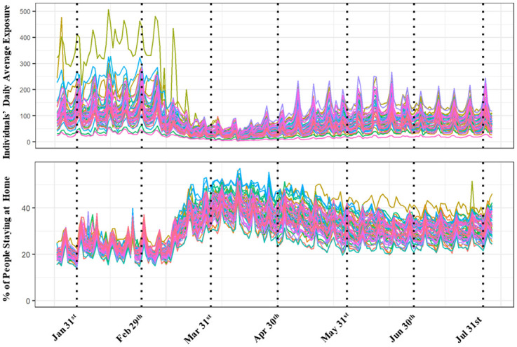
The second measure, information on social distancing is collected from Safegraph data (see Acknowledgement section for description of Safegraph data). These metrics provide information on the number of devices completely staying at home, mean/median distance travel from home, full time and part time work behavior at a daily basis for each county. Fig 2 provides a summary of both these measures at a state level from January 22nd to August 4th. From the figure, we can clearly see the reduction in average daily exposure in March as many states and local jurisdictions imposed lockdowns. By late April, exposure activity started to increase again across all the states while still being lower than the levels for February. In terms of the staying at home measure, as expected, we find an exactly opposite trend.
Fig 2. Average daily exposure and percentage of people staying at home.
Finally, within the healthcare infrastructure attributes, information about the hospitals and ICU beds are gathered from the County level health ranking data. COVID-19 testing measures are sourced from the COVID-19 tracking project [31] that provides a complete picture of testing as well the number of positive and negative cases for each county in the United States.
Dependent variables
We analyze two county level dependent variables: (1) COVID-19 daily transmission rate per 100K population and (2) COVID-19 mortality rates per 100K population. For the transmission rate analysis, we tested two alternative functional forms: daily cases per 100 thousand people and 7-day moving average of cases per 100 thousand people. The moving average data is likely to be less volatile and serves as a stability test for the daily cases model. The reader would note that we used a natural logarithmic transformation for all the dependent variables. The COVID-19 dataset from Center for Systems Science and Engineering (CSSE) Coronavirus Resource Center at Johns Hopkins University [32] provides information on the daily confirmed COVID-19 cases, number of people recovered (when available) and the number of deaths from COVID-19 starting from January 22nd to the current date across 3,142 counties in the United States. In our research, we confined our analysis to the cases between March 25th to August 4th resulting in 133 days of data. Further, we focus on counties that have at least 100 cases by August 4th and have available information on the mobility trends. With this requirement, a total of 1,752 counties are included in the analysis providing a coverage of 93% of the total population in the United States. For mortality rate, we considered the fatalities within the same time frame across all the 1,752 counties as the transmission rate variable. The summary statistics of the dependent variable are presented in bottom row panel of Table 1.
Data analysis (Modeling framework)
The two dependent variables: (a) COVID-19 daily transmission rate and (b) COVID-19 mortality rate are continuous in nature and linear regression model is the most traditional method to study such continuous responses. For the analysis of daily transmission rate, we have repeated measures of the variable (133 repetitions for each county). The traditional linear regression model is not appropriate to study data with multiple repeated observations [33]. Hence, we employ a linear mixed modeling approach that builds on the linear regression model while incorporating the influence of repeated observations from the same county. By adopting the linear mixed model, we recognize the dependencies across COVID-19 cases occurring for the same county. A brief description of the linear mixed model is provided below:
Let q = 1, 2, …, Q be an index to represent each county, and d = 1, 2, …, D be an index to represent the various days on which data (cases) was collected. The general form of the mixed linear regression model has the following structure:
| (1) |
where yqd is the dependent variable representing the new COVID 19 cases per 100K population, X is the vector of attributes and β is the model coefficients. εqd is the random error termassumed to be normally distributed across the dataset.
This ε term captures the dependencies across the repetition for each county. In our analysis, we estimate the correlation for different level of repetition measures: correlation for all records (133 repetitions), monthly level (31 repetitions) and weekly level (7 repetitions). The flexibility offered by the mixed model for testing dependencies enhances the model development exercise over its simpler form. In this structure, the data can be visualized as K (K = 133 or 31 or 7) records for each 1,752 counties. Estimating a full covariance matrix (up to 133*133) is computationally intensive while providing very little intuition. Hence, we parameterize the covariance matrix (Ω).
For estimating a parsimonious specification, we tested first-order autoregressive (AR) and autoregressive moving average (ARMA) correlation structure within the mixed linear model. The reader would note that the final model was identified based on three criteria: autocorrelation function (ACF); a partial autocorrelation function (PACF) and Bayesian Information Criterion metric (BIC). All of these measures provide support to the ARMA model selection (see S1 File for more details). Therefore, in the current study, we will only discuss the framework for the ARMA model (due to space constraints). The ARMA correlation structure comprises three parameters σ, ρ, and φ as follows:
| (2) |
where, σ represents the error variance of ε, φ represents the common correlation factor across time periods K, ρ represents the dampening parameter that reduces the correlation with time and K represents the level of repetition. The correlation parameters φ and ρ, if significant, highlight the impact of county effects on the dependent variables. The models are estimated in SPSS using the restricted maximum likelihood estimation (RMLE) approach. For modeling the COVID 19 mortality rate, we rely on simple linear regression approach as the dependent variable here is the total number of COVID-19 deaths per 100K population at a county level.
Results
The reader would note that prior to estimating the models, we checked for the multicollinearity issue across the independent variables as it is possible that county level characteristics are highly correlated. We did not find any significant impact of multicollinearity on our model estimates (see S1 File for more details).
COVID-19 transmission rate model results
The estimation results for the linear mixed model are presented in Table 2. From this point, we will use the term transmission rate for representing the natural logarithm of daily COVID-19 cases per 100K population. As discussed earlier, we also developed the same mixed linear model to estimate the 7-day moving average of COVID-19 cases per capita and find similar results as in the daily COVID-19 transmission model (results are available upon request from the authors). This further reinforces the stability of the transmission model.
Table 2. Estimation results for daily COVID-19 transmission rate per 100K population.
| Variables | Estimates | t-statistic | p-value |
|---|---|---|---|
| Constant | -4.882 | -18.307 | <0.001 |
| Demographics | |||
| % of Female population | 0.019 | 8.794 | <0.001 |
| % Young population (< = 18 years) | 0.009 | 6.097 | <0.001 |
| % of African-American population | 0.010 | 27.055 | <0.001 |
| % of People less than high school education | 0.022 | 22.738 | <0.001 |
| Ln (median income) | 0.325 | 14.185 | <0.001 |
| Employment rate per capita | 0.963 | 9.320 | <0.001 |
| Ln (% of People living in rural areas) | -0.408 | -17.567 | <0.001 |
| Health Indicators | |||
| Ln (HIV rate per 100K People) | 0.044 | 7.441 | <0.001 |
| Hepatitis C rate per 100K People | 0.012 | 3.200 | <0.001 |
| Mobility Trends | |||
| Ln (Daily Average Exposure), 10 days lag | |||
| April 25th to July 21st | 0.028 | 12.360 | <0.001 |
| After July 21st | 0.171 | 17.085 | <0.001 |
| % People staying at home (14 days lag) | |||
| March 25th to July 21st | -0.590 | -5.564 | <0.001 |
| After July 21st | -3.952 | -13.023 | <0.001 |
| Health Care Infrastructure Attributes | |||
| Ln (Testing), 5 days lag | |||
| March 25th to May 10th | 0.012 | 7.654 | <0.001 |
| After May 10th | 0.019 | 15.350 | <0.001 |
| Temporal Factors | |||
| Temporal Lagged Variables | |||
| 7 days lag (March 25th to June 22nd) | 0.177 | 69.165 | <0.001 |
| 7 days lag (June 23rd to July 6th) | 0.285 | 66.121 | <0.001 |
| 7 days lag (After July 6th) | 0.362 | 115.590 | <0.001 |
| 14 days lag | 0.167 | 77.272 | <0.001 |
| Day is Weekend | -0.045 | -10.695 | <0.001 |
| Correlation | |||
| σ | 0.988 | 275.252 | <0.001 |
| ρ | 0.959 | 367.088 | <0.001 |
| ϕ | 0.286 | 102.854 | <0.001 |
Socio-demographics
We find several socio-demographic variables to have significant impact on the transmission rate. In terms of female population, we find that higher proportion of females in the population has a positive impact on transmission rated. At first glance, the result might appear to be contradicting earlier studies that show women are less likely to be affected by COVID-19 transmission relative to men [18]. However, the reader would note that this result only implies that counties with higher percentage of female population are likely to experience increased number of COVID-19 cases relative to other counties. The finding does not necessarily indicate that women are at a higher risk of being infected by COVID-19. For differences in proclivity for COVID-19 infection by gender, individual level data would be a more appropriate avenue for analysis. Among age distribution proportions, we found that increased percentage of younger individuals (<18 years) is associated with more transmission. In terms of racial distributions, counties with higher proportion of African-Americans are likely to have higher transmission rates (see earlier work for similar findings [13, 20]). It has been postulated that African-Americans in general reside in densely populated low income neighborhoods with lower access to amenities and are employed in industries that requires more public exposure [19]. Educational status in a county also plays an important role in influencing the COVID-19 transmission. The counties with higher share of individuals with less than high school education are likely to report increased incidence of COVID-19. In terms of income, we find that higher median income in a county leads to rise in daily COVID-19 incidence. The effect of income might appear counter-intuitive at first glance. However, it is possible that higher income individuals are more likely to get tested (even in the absence of symptoms) due to higher health insurance affordability. Low income individuals are more likely to lose their jobs and health insurance coverage due to COVID-19 pandemic [13, 34]. With respect to employment rate, counties with higher employment rate reflect more exposure and have a positive association with transmission. The percentage of people living in rural area offers a negative association with the daily COVID-19 incidence. This indicates that people living in rural areas are less affected by COVID-19. This is intuitive as rural areas are sparsely populated and hence have more opportunity for social distancing thus lowering transmission rates.
Health indicators
With respect to health indicators, we tried several variables in the transmission rate model. Of these, two variables number of people suffering from HIV and hepatitis C in a county offered significant impacts. We observe that counties with higher percentage of HIV and hepatitis C patients have an increased incidence of COVID-19 transmission. Individuals with these diseases have weaker immune systems and hence are more susceptible to COVID-19 transmission.
Mobility trends
In terms of mobility trends, we tested two measures: daily average exposure and percentage of people staying at home. In considering these variables in the model, we recognize that exposure will have a lagged effect on transmission i.e. exposure to virus today is likely to manifest as a case in the next 5 to 14 days. In our analysis, we tested several lag combinations and selected the 10 day lag exposure as it offered the best fit. Similarly, for people staying at home, the 14 day lag offered the best fit. The exposure variable offers interesting results. Until April 25th exposure variable does not have any impact on transmission. This is strongly coinciding with the lower exposure trends (see Fig 2). After April 25th, increased exposure is associated with higher transmission rates 10 days into the future (see Hamada and colleagues [24] for similar findings). Further, the influence of exposure is substantially larger after July 21st indicating a higher risk of exposure for COVID-19 transmission. For the second measure, staying at home with 14 days lag, we find that daily transmission rates are negatively affected as expected [12, 21]. The impact of staying at home percentage is particularly stronger in recent weeks as indicated by the higher negative impact from July 21st. The two variable effects since July 21st reflect the influence of increased exposure to COVID-19 in recent weeks across the country. The reader would note that the two measures considered were not found to be strongly correlated (see S1 File for details) and thus were simultaneously considered in the model.
Health care infrastructure attributes
The only set of variables found to have a significant impact of COVID-19 transmission rate within this category correspond to COVID-19 testing effects. Again, we select a 5 day lag as we believe testing results are provided in 3–5 days. The coefficient of this variable is positive as expected and highly significant [21]. However, after May10th, the effect has a higher magnitude which suggests that compared to the previous time period (before May 10th), higher testing rate will increase the daily COVID-19 transmission at a marginally higher rate.
Temporal factors
With data available for 133 days, we can evaluate the effect of the transmission rate in previous time period on the current time period. As expected, we find a positive association between the daily COVID-19 transmission rate and the temporal lagged variables in the previous time period for 7 and 14 days. The result suggests higher transmission rate in previous time periods (7 and 14 days earlier) is likely to result in increased transmission. However, the effect is higher for the 7 day lagged variable, as evidenced by the higher magnitude associated with the corresponding time period in Table 2. Further, the 7 day lagged transmission rate after June 21st and July 7th time period offer larger positive impacts. Unsurprisingly, the effect for July 7th and later is significantly larger than the other variable effect. The result is aligned with the sudden surge in COVID-19 cases since beginning of July. Finally, the weekend variable highlights that the COVID-19 transmission rate is lower during weekends possibly because of reduced testing rate on weekends [35].
Correlation
As indicated earlier, we developed the mixed linear model for estimating the daily COVID-19 transmission rate per 100,000 people while incorporating the dependencies across each county for multiple repetition levels. Of these different models, we selected the model that provides best result in terms of statistical data fit and variable interpretation. We found that the model accommodating weekly correlations provided the best result. The final set of variables in Table 2 corresponds to the correlation parameter across every 7 days within a county. All the parameters are highly significant highlighting the role of common unobserved factors influencing the daily COVID-19 transmission rate over a week across the counties.
COVID-19 mortality rate
As opposed to the transmission rate model, we adopted a simple linear regression approach to study the determinants of the COVID-19 mortality rate at a county level. The coefficients in Table 3 represent the effect of different independent variables on the COVID-19 mortality rate (total number of deaths per 100K population in 3 months period) at a county level.
Table 3. Estimation results for COVID-19 mortality rate per 100K population.
| Variables | Estimates | t-statistic | p-value |
|---|---|---|---|
| Constant | -6.467 | -3.741 | <0.001 |
| Demographics | |||
| Older people % (>65 years old) | 0.053 | 6.663 | <0.001 |
| % of African-American population | 0.021 | 8.077 | <0.001 |
| % of People less than high school education | 0.070 | 10.730 | <0.001 |
| Income inequality ratio | 0.168 | 3.700 | <0.001 |
| Employment rate per capita | 6.381 | 7.953 | <0.001 |
| Ln (% of People living in rural areas) | -1.335 | -7.061 | <0.001 |
| Health Indicators | |||
| Ln (HIV rate per 100K people) | 0.200 | 4.889 | <0.001 |
| Cancer rate per 100K people | 0.256 | 1.919 | 0∙036 |
| Hepatitis A rate per 100K People | 0.051 | 2.157 | 0∙031 |
| Ln (Cardiovascular disease per 1K people) | 0.386 | 3.064 | 0∙002 |
| Health Care Infrastructure Attributes | |||
| ICU beds per capita | -0.007 | -4.382 | <0.001 |
Socio-demographics
With respect to socio-demographic variables, we find several attributes to have a significant impact on the COVID-19 mortality rate. For instance, higher percentage of older people in a county leads to an increased COVID-19 mortality rate as indicated by the positive coefficient in the Table 3. Similar results are also observed in earlier studies [16, 20]. Further, consistent with previous research [19], the current analysis also found a positive coefficient associated with the percentage of African-American people revealing a higher COVID-19 mortality rate in counties with higher proportion of African-American people. The variable specific to education status indicates that the likelihood of COVID-19 mortality increases with increasing share of people with less than high school education in a county. From the estimated results presented in Table 3, we find that counties with higher income inequality ratio are more likely to experience higher number of COVID-19 deaths per capita relative to the counties with lower income disparities. Higher income inequality mainly reflects a significant share of low-income workers who possibly need to continue their daily activities despite the risk of COVID-19 transmission. Further, they usually have less access to the health care system and thus have an increased risk of mortality [36]. Moreover, we find a positive association between the employment rate and COVID-19 mortality rate in a county. As discussed in the transmission model, high employment rate mainly reflects increased exposure which eventually increases the risk of COVID transmission resulting in higher risk of COVID-19 mortality. Finally, the last variable in the demographic category corresponds to the percentage of people living in rural areas that implies a negative effect on COVID-19 mortality rate indicating a reduced COVID-19 mortality rate in a county with more people living in the rural regions.
Health indicators
Among the health indicators, we found several variables significantly influence the COVID-19 mortality rate in a county. For instance, in comparison to other counties, counties with higher number of HIV, cancer, hepatitis A and cardiovascular patients are more likely to have higher number of COVID-19 deaths. This is expected as people with such conditions usually have weaker immune system which makes them vulnerable to the disease. The results are in line with a number of earlier studies [5, 37, 38].
Health care infrastructure attributes
Finally, among health care infrastructure attributes, number of ICU beds per capita at a county is found to have a negative impact on COVID-19 mortality rate suggesting a reduced death rate with higher number of ICU bed per person in a county. The result is intuitive as more ICU bed per capita indicates the county is well equipped to handle higher patient demand and treatment is accessible to more COVID-19 patients.
Policy implications
To illustrate the applicability of the proposed COVD-19 transmission model, we conduct a scenario analysis exercise by imposing hypothetical mobility restrictions. While earlier researchers explored the influence of mobility measures, these models did not account for county level factors such as socio-demographics, health indicators and hospital infrastructure attributes. In our framework, the sensitivity analysis is conducted while controlling for several other factors. The hypothetical restrictions on mobility are considered through the following changes to two variables:
county level average daily exposure reduced by 10%, 25% and 50%
county level percentage of stay at home population increased to 40%, 50% and 60%.
The changes to the independent variables were used to predict the transformed dependent variable. Subsequently, the transformed variable was converted to the daily cases per 100 thousand people. The results from this exercise are presented in Table 4. We present the average change in cases for all counties (1,752), and for the 100 counties with the highest overall transmission rates. From Table 4, two important observations can be made. First, changes to average daily exposure and stay at home population influence COVID-19 transmission significantly. In fact, by increasing stay at home population share to 50%, the model predicts a reduction of the number of cases by about 33%. Further, mobility restriction results in suppressed COVID-19 transmission as indicated by the negative values from Table 4. Second, the benefit from mobility restrictions and staying at home is slightly higher for the worst 100 counties with higher overall cases. The two observations provide evidence that issuing lockdown orders in counties with a recent surge is a potential mitigation measure to curb future transmission.
Table 4. Policy scenario analysis of social distancing in COVID-19 transmission rate per 100K population.
| Hypothetical Scenarios | 1,752 Counties | Worst 100 Counties |
|---|---|---|
| 1: daily average exposure reduced by 10% | -0.636 | -0.640 |
| 2: daily average exposure reduced by 25% | -1.716 | -1.726 |
| 3: daily average exposure reduced by 50% | -4.030 | -4.055 |
| 4: 40% people stay at home | -26.423 | -26.654 |
| 5: 50% people stay at home | -33.082 | -33.258 |
| 6: 60% people stay at home | -38.561 | -38.700 |
The COVID-19 total mortality rate model can be employed to identify vulnerable counties that need to be prioritized for vaccination programs (when available). While prioritizing the counties based on mortality rate might be a potential approach, it might be feasible. To elaborate, vaccination programs have to be planned well in advance (say 2 months) of the vaccine availability. As total mortality rates for 2 months into the future are unavailable, we need a model to predict total mortality into the future. The estimated mortality rate model provides a framework for such analysis. To be sure, it would be prudent to update the proposed model with the latest data to develop a more accurate prediction system.
Discussion
The current study develops a comprehensive framework for examining COVID-19 transmission and mortality rates in the United States at a county level including an exhaustive set of independent variables: socio-demographics, health indicators, mobility trends and health care infrastructure attributes. In our analysis, we consider all counties with total number of cases greater than 100 on August 4th and analyze daily cases data from March 25th to August 4th, 2020. The COVID-19 transmission rate is modeled at a daily basis using a linear mixed method while the total mortality rate is analyzed adopting a linear regression approach.
Several county level factors including proportion of African-Americans, income inequality, health indicators associated with Asthma, Cancer, HIV and heart disease, percentage of stay at home individuals, testing infrastructure and Intensive Care Unit capacity impact transmission and/or mortality rates. The results clearly support our hypothesis of considering a universal set of factors in analyzing the COVID-19 data. Further we conducted policy scenario analysis to evaluate the influence of social distancing on the COVID-19 transmission rate. The results highlight the effectiveness of social distancing in mitigating the virus transmission. In fact, we found that by increasing stay at home population share to 50% the model predicts a reduction of the number of cases by about 33%. The finding provides evidence that issuing lockdown orders in counties with a recent surge is a potential mitigation measure to curb future transmission.
To be sure, the study is not without limitations. The study is focused on county level analysis and is intended to reflect associations as opposed to causation. However, for the causation based analysis, data from individuals would be more suitable. As with any area level analysis, there is a small possibility that some of the estimated parameters might be spurious associations due to aggregation bias. However, in the absence of individual level data, these area level models offer a valid and useful tool for epidemiologists and planners. Further, the inherent aggregation of the data at a county level would initiate some form of spatial heterogeneity which we did not account for in our analysis. In future, it would be interesting to accommodate these effects separately while considering the temporal correlation. Further, the proposed model can be enhanced using more detailed information such as percentage of health workers in the workforce, number of hospital beds and mask mandate dates. While exposure data were reasonably addressed, data was not available for mask wearing behavior across all counties. Finally, the data on transmission and mortality are updated for few counties to correct for errors or omissions. These were carefully considered in our data preparation. However, it is possible that further updates might be made after we finished our analysis.
Supporting information
(PDF)
Acknowledgments
The authors would like to gratefully acknowledge SafeGraph COVID-19 Data Consortium, County Health Ranking and Road Maps, Centers for Disease Control System for providing access to the data at county level for United States. SafeGraph is a data company that aggregates anonymized location data from numerous applications in order to provide insights about physical places. To enhance privacy, SafeGraph excludes census block group information if fewer than five devices visited an establishment in a month from a given census block group.
Data Availability
All relevant data are within the manuscript.
Funding Statement
The author(s) received no specific funding for this work.
References
- 1.Worldometer. Coronavirus Cases & Mortality [Internet]. Worldometer. 2020 [cited 2020 Jul 12]. p. 1–22. https://www.worldometers.info/coronavirus/?
- 2.The Global Economic Outlook During the COVID-19 Pandemic: A Changed World [Internet]. [cited 2020 Jul 12]. https://www.worldbank.org/en/news/feature/2020/06/08/the-global-economic-outlook-during-the-covid-19-pandemic-a-changed-world
- 3.Bhowmik T, Eluru N. A Comprehensive County Level Framework to Identify Factors Affecting Hospital Capacity and Predict Future Hospital Demand. [cited 2021 Mar 9]; Available from: 10.1101/2021.02.19.21252117. [DOI] [PMC free article] [PubMed] [Google Scholar]
- 4.Centers for Disease Control and Prevention (CDC). Cases in the U.S. [Internet]. Vol. 2019, Coronavirus Disease 2019 (COVID-19). 2020 [cited 2020 Jul 12]. p. 1–4. https://www.cdc.gov/coronavirus/2019-ncov/cases-updates/cases-in-us.html?CDC_AA_refVal=https%3A%2F%2Fwww.cdc.gov%2Fcoronavirus%2F2019-ncov%2Fcases-updates%2Fsummary.html%0Ahttps://www.cdc.gov/coronavirus/2019-ncov/cases-updates/cases-in-us.html
- 5.Bansal M. Cardiovascular disease and COVID-19. Diabetes Metab Syndr Clin Res Rev. 2020;14(3):247–50. [DOI] [PMC free article] [PubMed] [Google Scholar]
- 6.Engle S, Stromme J, Zhou A. Staying at Home: Mobility Effects of COVID-19. SSRN Electron J. 2020; [Google Scholar]
- 7.Mukandavire Z, Nyabadza F, Malunguza NJ, Cuadros DF, Shiri T, Musuka G. Quantifying early COVID-19 outbreak transmission in South Africa and exploring vaccine efficacy scenarios. PLoS One. 2020;15(7 July):e0236003. 10.1371/journal.pone.0236003 [DOI] [PMC free article] [PubMed] [Google Scholar]
- 8.Yuan X, Xu J, Hussain S, Wang H, Gao N, Zhang L. Trends and Prediction in Daily New Cases and Deaths of COVID-19 in the United States: An Internet Search-Interest Based Model. Explor Res Hypothesis Med. 2020;000(000):1–6. 10.14218/ERHM.2020.00023 [DOI] [PMC free article] [PubMed] [Google Scholar]
- 9.Courtemanche CJ, Garuccio J, Le A, Pinkston JC, Yelowitz A. Did Social-Distancing Measures in Kentucky Help to Flatten the COVID-19 Curve? Inst study Free Enterp Work Pap [Internet]. 2020;4:1–23. Available from: https://uknowledge.uky.edu/isfe_papers%0Ahttps://uknowledge.uky.edu/cgi/viewcontent.cgi?article=1000&context=isfe_papers [Google Scholar]
- 10.Zhan C, Tse CK, Lai Z, Hao T, Su J. Prediction of COVID-19 spreading profiles in South Korea, Italy and Iran by data-driven coding. PLoS One. 2020;15(7 July). 10.1371/journal.pone.0234763 [DOI] [PMC free article] [PubMed] [Google Scholar]
- 11.Ci C, Zhou B, Xi L. A support vector machine based scheduling approach for a material handling system. In: Proceedings—2010 6th International Conference on Natural Computation, ICNC 2010. 2010. p. 3768–72.
- 12.Bilgin NM. Tracing COVID-19 Spread in Italy with Mobility Data. SSRN Electron J. 2020; [Google Scholar]
- 13.Mollalo A, Vahedi B, Rivera KM. GIS-based spatial modeling of COVID-19 incidence rate in the continental United States. Sci Total Environ. 2020;728. 10.1016/j.scitotenv.2020.138884 [DOI] [PMC free article] [PubMed] [Google Scholar]
- 14.Sharkey P, Wood G. The Causal Effect of Social Distancing on the Spread of SARS-CoV-2. 2020; [Google Scholar]
- 15.Wu X, Nethery RC, Sabath BM, Braun D, Dominici F. Exposure to air pollution and COVID-19 mortality in the United States: A nationwide cross-sectional study. medRxiv Prepr Serv Heal Sci. 2020; 10.1101/2020.04.05.20054502 [DOI] [PMC free article] [PubMed] [Google Scholar]
- 16.Wieland T. Flatten the Curve! Modeling SARS-CoV-2/COVID-19 Growth in Germany on the County Level. medRxiv [Internet]. 2020;2020.05.14.20101667. Available from: http://medrxiv.org/content/early/2020/05/19/2020.05.14.20101667.abstract [Google Scholar]
- 17.Xie J, Zhu Y. Association between ambient temperature and COVID-19 infection in 122 cities from China. Sci Total Environ. 2020;724. 10.1016/j.scitotenv.2020.138201 [DOI] [PMC free article] [PubMed] [Google Scholar]
- 18.Borjas GJ. Demographic Determinants of Testing Incidence and COVID-19 Infections in New York City Neighborhoods. SSRN Electron J. 2020; [Google Scholar]
- 19.Backer A. Why COVID-19 May Be Disproportionately Killing African Americans: Black Overrepresentation among COVID-19 Mortality Increases with Lower Irradiance, Where Ethnicity Is More Predictive of COVID-19 Infection and Mortality Than Median Income. SSRN Electron J. 2020; [Google Scholar]
- 20.Xie Z, Li D. Health and Demographic Impact on COVID-19 Infection and Mortality in US Counties [Internet]. Medrxiv. 2020. Available from: 10.1101/2020.05.06.20093195 http://medrxiv.org/cgi/content/short/2020.05.06.20093195 [DOI] [Google Scholar]
- 21.Berger D, Herkenhoff K, Mongey S. An SEIR Infectious Disease Model with Testing and Conditional Quarantine. SSRN Electron J. 2020; [Google Scholar]
- 22.Teslya A, Pham TM, Godijk NG, Kretzschmar ME, Bootsma MCJ, Rozhnova G. Impact of self-imposed prevention measures and short-term government-imposed social distancing on mitigating and delaying a COVID-19 epidemic: A modelling study. PLoS Med. 2020;17(7):e1003166. 10.1371/journal.pmed.1003166 [DOI] [PMC free article] [PubMed] [Google Scholar]
- 23.Siedner MJ, Harling G, Reynolds Z, Gilbert RF, Haneuse S, Venkataramani AS, et al. Social distancing to slow the US COVID-19 epidemic: Longitudinal pretest–posttest comparison group study. PLoS Med [Internet]. 2020;17(8 August):2020.04.03.20052373. Available from: http://medrxiv.org/lookup/doi/10.1101/2020.04.03.20052373 [DOI] [PMC free article] [PubMed] [Google Scholar]
- 24.Badr HS, Du H, Marshall M, Dong E, Squire MM, Gardner LM. Association between mobility patterns and COVID-19 transmission in the USA: a mathematical modelling study. Lancet Infect Dis. 2020; 10.1016/S1473-3099(20)30553-3 [DOI] [PMC free article] [PubMed] [Google Scholar]
- 25.Omori R, Mizumoto K, Chowell G. Changes in testing rates could mask the novel coronavirus disease (COVID-19) growth rate. Int J Infect Dis. 2020;94:116–8. 10.1016/j.ijid.2020.04.021 [DOI] [PMC free article] [PubMed] [Google Scholar]
- 26.Triantaphyllou E, Sánchez A. A sensitivity analysis approach for some deterministic multi-criteria decision-making methods. Decis Sci. 1997; [Google Scholar]
- 27.Rehman S, A S. Multi-Criteria Wind Turbine Selection using Weighted Sum Approach. Int J Adv Comput Sci Appl. 2017; [Google Scholar]
- 28.Mateo JRSC. Weighted sum method and weighted product method. In: Green Energy and Technology. 2012. [Google Scholar]
- 29.USA Counties | ArcGIS Hub [Internet]. [cited 2020 Dec 11]. https://hub.arcgis.com/datasets/48f9af87daa241c4b267c5931ad3b226_0
- 30.Couture V, Dingel JI, Green A, Handbury J, Williams KR. Measuring Movement and Social Contact With Smartphone Data: a Real-Time Application To Covid-19 [Internet]. Vol. No. 27560, NBER Working Paper Series. 2020. Report No.: 35. http://www.nber.org/papers/w27560%0Ahttp://www.nber.org/papers/w27560.pdf
- 31.The COVID-19 tracking project [cited 2020 June 12]. https://covidtracking.com/data/.
- 32.COVID-19 Map—Johns Hopkins Coronavirus Resource Center [cited 2020 Jul 11]. https://coronavirus.jhu.edu/map.html
- 33.Faghih-Imani A, Eluru N, El-Geneidy AM, Rabbat M, Haq U. How land-use and urban form impact bicycle flows: Evidence from the bicycle-sharing system (BIXI) in Montreal. J Transp Geogr. 2014;41:306–14. [Google Scholar]
- 34.Ahmed F, Ahmed N, Pissarides C, Stiglitz J. Why inequality could spread COVID-19. Vol. 5, The Lancet Public Health. 2020. p. e240. 10.1016/S2468-2667(20)30085-2 [DOI] [PMC free article] [PubMed] [Google Scholar]
- 35.Reduced testing suggested as reason for weekend drop in confirmed COVID-19 deaths | Michigan Radio [cited 2020 Jul 11]. https://www.michiganradio.org/post/reduced-testing-suggested-reason-weekend-drop-confirmed-covid-19-deaths
- 36.Income and wealth inequality in the U.S. has fueled COVID-19 deaths—MarketWatch [cited 2020 Jul 11]. https://www.marketwatch.com/story/income-and-wealth-inequality-in-the-us-has-fueled-covid-19-deaths-2020-06-29
- 37.Common Questions About the New Coronavirus Outbreak [cited 2020 Jul 11]. https://www.cancer.org/latest-news/common-questions-about-the-new-coronavirus-outbreak.html
- 38.Zhang L, Zhu F, Xie L, Wang C, Wang J, Chen R, et al. Clinical characteristics of COVID-19-infected cancer patients: a retrospective case study in three hospitals within Wuhan, China. Ann Oncol. 2020;31(7):894–901. 10.1016/j.annonc.2020.03.296 [DOI] [PMC free article] [PubMed] [Google Scholar]
Associated Data
This section collects any data citations, data availability statements, or supplementary materials included in this article.
Supplementary Materials
(PDF)
Data Availability Statement
All relevant data are within the manuscript.