A Simplified Model for Simulating Population Responses of Tactile Afferents and Receptors in the Skin

Abstract

Tactile information about an object can only be extracted from population responses of tactile receptors and their afferents. Thus, to best control tactile information in robots, neuroprostheses or haptic devices, inputs should represent responses from full populations of afferents. Here, we describe a simplified model that recreates afferent population responses of thousands of tactile afferents in a personal computer. The whole model includes a resistance network model to simplify the skin mechanics and an improved version of a single unit model that we have previously described. The whole model was implemented by short and efficient python code. The parameters of the model were fit based on a simple vibrating stimulus, but the simulated outputs generalize to match receptive field sizes, edge enhancement, and neurophysiological responses to dot textures, embossed letters and curved surfaces. We discuss how to use this work to model haptic perception and provide guidance in designing and controlling highly realistic tactile interfaces in robots, neural prostheses and haptic devices.

I. Introduction

Tactile information is conveyed from the skin via 5 main afferent fiber types: the slowly adapting type 1 (SA1), the slowly adapting type 2 (SA2), the rapidly adapting type 1 (RA1), the Pacinian corpuscle (PC) and the C tactile (CT) [1]. Each afferent is associated with a different class of tactile receptor. There is strong evidence suggesting that discrimination of object properties such as edge orientation [2], shape [3], roughness [4], and texture [5], is based on the population responses of 3 of these afferent types: SA1, RA1 and PC [6, 7]. Present electrophysiological techniques limit our ability to record the responses of populations of tactile afferents, so a rapid and accurate model of afferent population responses would be an invaluable tool for controlling tactile devices, such as neural prostheses or robots, and to investigate the mechanisms underlying the tactile perception. The goal of the current work was to produce a model to recreate an afferent population response based on the response data of single afferents, which could generalize to recreate most response properties observed in the neurophysiological literature, while being simple enough to allow for fast computation, thus being appropriate for real-time control of neural prostheses or haptic devices.

Several studies have shown the viability of modeling single tactile afferents [8, 9], but there are very few studies that have simulated population responses [10–12]. Using an integrate-and-fire (IF) model and a continuum skin mechanic model, Saal et al developed a systematic model called TouchSim to simulate population responses [13]. It successfully reproduced afferent population responses to stimuli such as vibrating probes and tactile texture. The parameters of the TouchSim model were optimized manually using pattern search and genetic algorithms in Matlab [13]. The advantage of the TouchSim model is that it is able to reproduce precise temporal patterns of afferent activity, in part due to the complexity of the skin mechanics model. However, that complexity leads to slower processing with more complex stimuli. Indeed, while previous studies have adopted skin mechanics models [11, 12] or combined them with single-unit models to reproduce the population response [13–15], a precise model of skin mechanics requires many measured parameters and is time consuming. As such, a main aim of this work was to create a simplified skin mechanics model that would allow for fast processing even with complex stimuli.

Population responses of tactile afferents can be attributed to external factors (e.g. the stimulus or contact force) and internal factors (e.g., the mechanics of the skin and the arrangement of tactile receptors and their afferents). From the standpoint of internal factors, a stimulus applied to the skin will cause skin deformation around the stimulus site. We hypothesized that the pattern of indentation around a stimulus could be efficiently recreated by the pattern of node voltages in a resistance network. Based on this, we proposed that the skin can be treated as multiple nodes connected in a resistance network.

Histological studies have also revealed that afferents branch, with single afferent fibers innervating multiple receptors [16], which can yield complex receptive field with multiple hotpot [17]. We propose that to simulate afferent population responses, we only need to calculate indentation depths at sites of the tactile afferents, rather than for each receptor. Indeed, our model treats the combination of the receptors and associated afferent as a single unit for simplification.

Our resultant model utilized a skin contact model to generate input currents for the resistance network model. Single unit activity was generated using an improved version of our two channel-filter (TCF) model, and an IF neuron model converted the output to action potentials. The model was fitted automatically using neural data recorded from single afferents to vibrating probes and then tested with an array of tactile stimuli. The resultant model replicates neurophysiological response properties to many forms of tactile stimuli and runs in real time with about 2700 units at sampling rate of 300 Hz in Python.

II. Methods

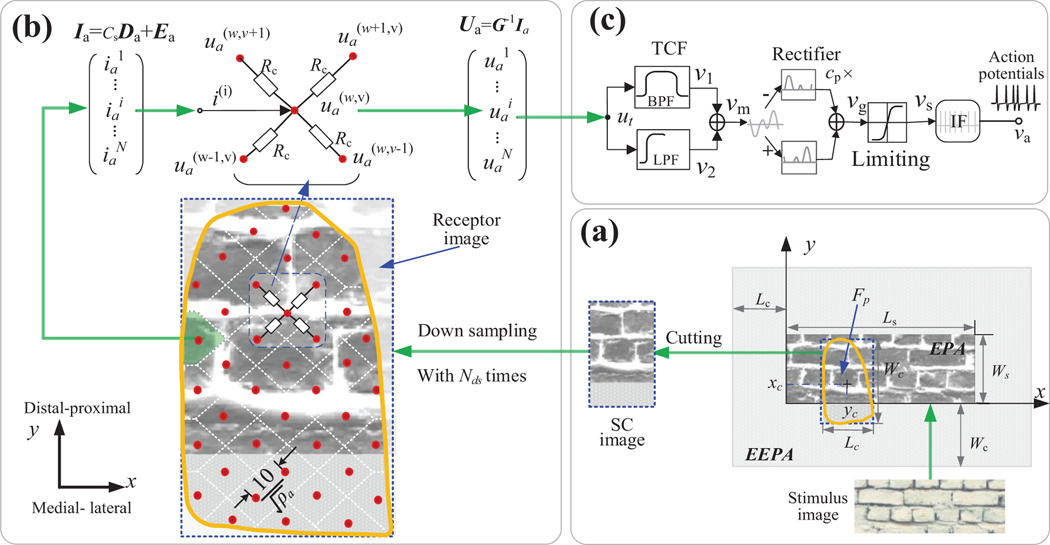
The whole model is comprised of a simplified skin contact model (Fig 1a), a resistance network model (Fig. 1b) and models of single tactile afferents (Fig 1c). As guided by the green arrows, the stimulus was constructed into an equivalent probe array (EPA). The part of the EPA in contact with the skin was defined as the SC (skin contact) image, which was then down-sampled into a receptor image. To generate the currents inputted into the resistance network, we covered a fixed area in the receptor image for each afferent as shown in the blue dotted box in Fig. 1b. Then we constructed the impedance matrix (G) of the resistance network to compute the node voltages. Finally, a single unit model was implemented to convert the node voltages to action potentials.

Fig. 1.

Schematic of the whole model. (a) Simplified skin contact (SC) model based on image. (b) The resistance network model of connecting all sampled tactile afferents in fingertip skin area shown as yellow curve box. In the skin area of fingertip, each red dot represents an afferent (node) and was connected by 4 resistors. The white dotted lines in skin area represent the boundaries for dividing the receptor image into several a small area for each tactile afferent in skin area. (c) Model of the single-unit.

The quantifying interaction between the EPA and skin (section 2A2), computing input currents and output voltages of the resistance network (section 2B3), and the filter model of single-unit (section 2C) are treated as the running model since they are changing when interacting with objects. Other parts of model (described in section 2A1, 2B1 and 2B2 below) were set in the initial stage in simulation since they can be treated as constant when interacting with hard stimuli. The core code of simulation model, all the variables and a link to the code on GitHub can be found in the supplementary Methods.

A. A simplified skin contact model

1). Constructing the EPA

An objective stimulus can be defined as a set of probes indented into the skin, orthogonal to the skin surface [13]. In this model, each probe has a diameter (D_bp) of 0.2 mm. We create each stimulus by setting probe heights (which will be converted to depth of indentation) across the EPA. Because the probes create a continuous array, a flat surface can be created by having neighboring probes of the same height. Supposed that L_s and W_s is length and width of the external rectangle of a stimulus surface. The EPA is characterized as a matrix with dimension of m×n:

$$\mathit{EPA}={\left(h_{ij}\right)}_{\text{m}\times \text{n}}i\in [1,2,\dots ,m],j\in [1,2,\dots ,n]$$ (1)

Where $m=\mathit{int}\left(W_s/D_{bp}\right),n=\mathit{int}\left(L_s/D_{bp}\right)$. As noted above, D_bp is the diameter of the probe. In order to ensure that all positions in the stimuli can be scanned by the skin area, we expand the EPA image with a distance equivalent to the width of the skin contact area (L_c) on the medial and lateral sides and by the length of the skin contact area (W_c) on the distal and proximal sides. Across this expanded area, probe height (hⁱ) is set to zero, as shown by the grey blank area in Fig 1a. The resultant larger image is called the extended EPA (EEPA).

The model is also able to create a tactile representation from a visual image, which can be used to construct natural texture EPAs. In this case, we extract height information according to the pixel value from the image after gray-scaling and normalizing. The image is then resized to a lower resolution to create the EPA image.

2). Quantifying the interaction between stimuli and skin

We directly computed skin indentation depths as input for the resistance network. After constructing the EEPA and the image, the indentation depths vector for inputs of the resistance network can be easily calculated by scanning the SC image across the EEPA image frame by frame as illustrated in Fig 1a. To characterize the scanning process between the SC image and the EEPA image, we defined a vector to quantify the input interaction vector (IV) parameters:

$$\mathit{IV}=\left(\begin{array}{c}{x}_c{y}_c{D}_p\end{array}\right)$$ (2)

Where the x_c, y_c (mm) is the contact position skin area center relative to EPA. The third parameter in the vector IV is D_p (the depth that the stimulus indents into the skin), which is the equivalent of F_p (the force that the stimulus applies to the skin).

The final receptor image was down sampled by a factor (N_ds) times from the SC image. N_ds was set to 1 for SA1, 1 for RA1, and 2 for PC afferents.

B. Resistance network model

1). Characterizing the distribution of tactile afferents and their coverage area in the receptor image

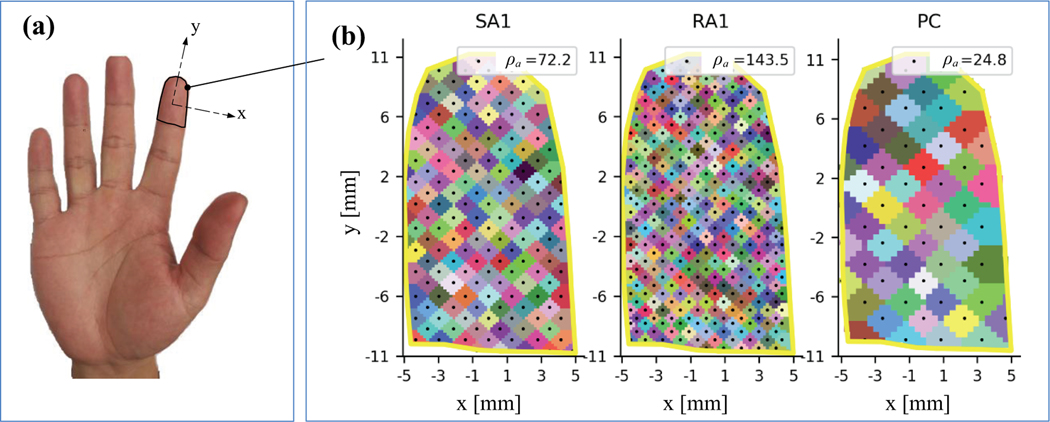
To characterize the distribution of tactile afferents, the locations of all the tactile afferents in the skin were arranged evenly over the sampled area according to afferent densities (ρ_a units/cm²). The ρ_a of the three classes of afferents were taken from [18], as shown in Fig. 2. To ensure that stimuli at any site on the finger can activate at least one tactile afferent, we attributed each pixel in the receptor image to a tactile afferent according to the its closest distance relative to the afferent site. ES₁, ES₂, listed in table 1, is the N×N_a matrixes of row and column entries of covering pixels in the receptor image for all tactile afferents respectively. N_a can be estimated according to the afferent density and D_bp (100/(ρ_a×D_bp²)). As illustrated in Fig 2b, using the two matrixes we create a clear diamond area in the receptor image for each of the tactile afferents in the fingertip.

Fig. 2.

(a) The sampled skin area in fingertip selected from a real human hand of a man. (b) Distribution of tactile afferents and their covering areas (colored blocks) in receptor image. The black dot localizing at the center of each covering area represent the site of each tactile afferent.

2). Constructing the impedance matrix of the resistance network

As described above, we chose to simplify the skin mechanics by treating the afferent population as a set of tactile afferents of the same class connected in a resistance network. Here we describe how we constructed the impedance matrix to generate input voltages for the single-unit model shown in next section.

The template resistance network is illustrated in Fig. 1b. The evoked activity from the targeted unit is conducted to adjacent tactile afferents of same type through 4 identical resistors, with R_c as the resistance of each resistor. According to the Thevenin node voltage equation, the connection voltage $u_a^{(w,v)}$ of entry (w, v) is given as:

$$\begin{gathered} \frac{1}{C_d}\cdot \frac{4}{R_{\text{C}}}\cdot u_a^{(w,v)}-\frac{\left(u_a^{(w-1,v)}+u_a^{(w+1,v)}\right)}{R_{\text{c}}}-\frac{\left(u_a^{(w,v-1)}+u_a^{(w,v+1)}\right)}{R_{\text{c}}} \\ =i_a^{(w,v)}w,v\in (\dots -2,-1,0,1,2,\dots ) \end{gathered}$$ (3)

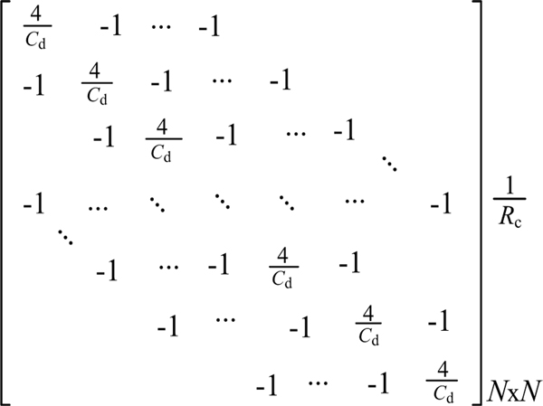
Where C_d is the conductivity of the resistance network C_d (<2), which can be used to characterize the different RF sizes for different afferent types. The connection voltages (u_as) of all nodes in the two-dimensional network were converted to a column vector (U_a). The impendence matrix (G) was determined from the left side of equation (3). This results in the N×N matrix shown in Fig. 3, where N is the number of tactile afferents.

Fig. 3.

Matrix of resistance network of 164 SA1 tactile afferents in fingertip area

3). Generating input currents and output voltages of the resistance network

The input current for each tactile afferent was computed from pixels values in its covered area resulting in a vector of depths indented into the skin at all afferent sites (D_a). D_a is computed from receptor image using the matrix ES₁, ES₂, and D_p as illustrated in step 5 in the supplementary Methods. If the third parameter in IV is force signal, D_p (The depth that the stimulus indents into the skin) can also be calculated as a function of the contact force (F_p) according to elasticity theory

$$D_p=\frac{\left(1-{ϵ}^2\right)\cdot F_{\text{p}}}{2\cdot E\cdot r_{\text{p}}},r_{\text{p}}=\sqrt{\frac{n\cdot \pi \cdot {\left(D_{\text{bp}}\cdot N_{\text{ds}}/2\right)}^2}{\pi }}$$ (4)

Where n is the total number of pixels in receptor image with values higher than 0. E and ε is the Young’s module and Poisson constant respectively.

As illustrated in Fig. 1a, the inputting node current vector $\left({\mathit{I}}_{\text{a}}=\left[i_{\text{a}}^1,i_{\text{a}}^2,\dots ,i_{\text{a}}^N\right]\right)$ for all the tactile afferents connected in the resistance network was obtained by:

$$\{\begin{array}{c}{\mathit{I}}_{\text{a}}=C_{\text{S}}\cdot {\mathit{D}}_{\text{a}}+{\mathit{E}}_{\text{a}}\\ {\mathit{E}}_{\text{a}}=C_{\text{e}}\cdot {\mathit{D}}_{\text{a}}\cdot {\mathit{var}}_{-}r\left(\mathit{R}\mathit{I}\left[\mathit{E}{\mathit{S}}_1,\mathit{E}{\mathit{S}}_2\right]\right)\end{array}$$ (5)

Where C_s is a constant coefficient of converting D_a to current. The vector E_a was used to emulate edge enhancement and C_e is the coefficient of edge enhancement. “var_r()” represents the function of computing variance of a matrix by rows. E_a was obtained by computing the variation of the matrix after substituting the ES₁ and ES₂ to RI by rows. Previous studies have indicated that the receptive field (RF) is strongly related to afferent branching. By incorporating ES₁ and ES₂ in the E_a, we may improve the performance of simulating afferent response properties such as RF size.

The node voltage vector for all the tactile afferents connected in each resistance network (U_a) can be calculated by substituting the current vector (I_a) in following equation.

$${\mathit{U}}_a={\mathit{G}}^{-1}\cdot {\mathit{I}}_a$$ (6)

Where G⁻¹ is the inverse matrix of G. According to equations (5), (6) and Fig. 3, the response of the i^th tactile afferent to the probe are positively related by $R_{\text{c}}\cdot {\mathit{G}}^{-1}(i,i)\cdot i_{\text{a}}^i$. Therefore the parameters of the resistance network are strongly reflected in the responses of the single units. That is why the parameters of resistance network can be fitted by response data of single units to vibrating probe.

C. Modelling single-unit

In the single unit model, the voltage of each node in the resistance network is processed by a two-channel filter, in which the low-pass and band pass fitters were designed to mimic the static and dynamic aspects of stimulus indentation respectively. Three afferent types are modeled using a common circuit shown in Fig 1c. In our previous work [9], we showed that the selective responses of RA1, SA1 and PC afferents can be modeled using a two-channel filter (TCF) model. Here, we simplified our previous TCF model to quantitatively replicate the selective responses of the tactile afferents, then constructed an IF neuron model to output action potentials. The Laplace transfer function of the TCF model is given as below.

$$H_{(s)}=\frac{v_m(S)}{u_a(S)}=\underset{\text{BPF}}{\underbrace{\frac{K_{b1}\cdot \frac{2\pi \cdot f_b}{Q}\cdot S+K_{b2}\cdot S^2}{S^2+\frac{2\pi \cdot f_b}{Q}S+4{\pi }^2\cdot f_b^2}\cdot \frac{2\pi \cdot f_b}{S+2\pi \cdot f_b}}}+\underset{\text{LPF}}{\underbrace{\frac{K_u\cdot 2\pi \cdot f_l}{S+2\pi \cdot f_l}}}$$ (7)

Where u_a and v_m are the input and output signals of the TCF model, respectively. f_b (Hz), Q and f_l (Hz) are the center frequency of the BPF, the quality factor of the BPF and the cutoff frequency of the LPF, respectively. The above transfer function can be discreetly solved by a differential equation as shown in in step 5 in the supplementary Methods. Because afferents tend to respond differently to stimulus onsets and offsets [19], we incorporated a weighted rectifier (c_p) that was set to 0 for SA1 afferents and to a value between 0 and 1 for RA1 and PC afferents.

There are several commonly used spiking neuron models, such as the Hodgkin-Huxley model [20] and other more simplified models: Morris-Lecar model, and Integrate-and-fire (IF) [21, 22]. We used a leaky IF neuron model which has computational simplicity and applicability to simulate SA1, RA and PC afferents [23, 24]. The mean firing rate of the neuron changes with the input voltage of the IF neuron model and can be given as follows according to the literature [25].

$$f_r=\frac{1}{-\tau \cdot ln\left(1-\frac{v_{th}}{v_S}\right)}\sim \frac{1}{\tau }\cdot \frac{v_S}{v_{th}}{v}_S\gg v_{th}$$ (8)

To reflect the saturation of the single afferent response, we limit vs to a range with an upper limit of $V_{\text{H}}=f_{\text{rmax}}\cdot V_{\text{th}}\cdot \tau .f_{\text{rmax}}$ is the maximum firing rate, and was set to 120, 200, 300 for SA1, RA1 and PC units respectively.

D. Model fitting

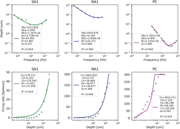
We designed two steps for fitting the parameters automatically using response data of single-units to sinusoidal vibration. The first step mainly focused on fitting the single-unit parameters (e.g., f_b, K_u, K_b1) using a neural threshold (D_th, um)-frequency (f) electrophysiological data (extracted from Figure 7 in reference [26]). The second stage mainly focused on fitting the parameters of the resistance network model (e.g., C_s R_c, c_p) using firing-rate (f_r)-depth amplitude (d_m, um) electrophysiological data (extracted from the first column of Figure 4 in reference [7]) The objective function for fitting parameters of the single-unit model is illustrated in the following equation.

Fig. 4.

Results of fitting parameters of single-unit (top) and population (bottom). Data points show the recorded data and the colored lines show the fit of the model.

$$D_{\text{th}}=\frac{V_{th}}{K_n\cdot |H(j\cdot 2\pi \cdot f)|}$$ (9)

Where D_th is the minimum indentation depth to activate a single tactile afferent.

Since the frequency characteristics of the model were determined after the fitting in the first stage, we can fit the population parameters with neural data of firing-rates as a function of depth under a single frequency. We select neural data under near the central frequencies (50, 100, 300Hz) for fitting the SA1, RA1 and PC models respectively. The firing rate of each tactile afferent is almost linear with the input voltage of the IF model as illustrated in equation (8). The variance value in equation (5) for each afferent type can be computed by the area of the probe in the reference [7] (0.25π mm²), and afferent density. Therefore the function of fitting the population parameters using firing-rate data changed as a function of depth can be evaluated as follows:

$$\{\begin{array}{c}{f}_r\left(d_m\right)=\frac{\frac{1}{4}{c}_d\cdot R_C\cdot \frac{1}{\tau }\cdot \frac{1+w}{\pi }\left(C_s+C_e\cdot \text{var}\right)\cdot d_m}{K_n\cdot D_{th}(f)}f\in [50,100,300\text{Hz}]\\ f_r\left(d_m\right)=f_{\text{rmax}}{f}_r\left(d_m\right)>f_{\text{rmax}}\end{array}$$ (10)

Where f_r is the firing rate (spikes/s) The lower boundaries of all the parameters were set to zero. We adopted a typical least squares fitting method using the Curve_fit module in the Scipy.optimize library. In order to visualize whether the model parameters were correctly fitted to match with original neural data, we present fitting curves for the first fitting step (Fig. 4, top panels) and the second fitting step (Fig. 4, bottom panels), which show the D_th under different frequencies and f_r under different depths respectively. The gray points show the original neural data and the colored lines show the fitted output. Note that the data are very well fit, with R²s greater than 0.95 for the first fitting step and greater than 0.92 for the second fitting step.

The conductivity of the resistance network (C_d; listed in the lower panels of Fig 4), which can be used to get a rough estimate of receptive field size, is smallest for SA1s, greater for RA1s, and greatest for PCs. For SA1s, K_b1 is much high than K_u, which is in accordance with a previous conclusion that SA1 afferents respond about ten times more during dynamic stimulation than during static stimulation [27]. $Q_{(\text{PC})}>Q_{(\text{RAl})}>Q_{(\text{SAl})}$, and $f_{\text{b}(\text{PC})}>f_{\text{b}(\text{RA}1)}>f_{\text{b}(\text{SAl})}$, indicate that our PC units are more sensitive to the stimulus frequency than our RA1 and SA1 units, which also matches well with the characteristics of the 3 afferent types. The non-free parameters: f_rmax, E, and D_a were set based on the literature [7, 12, 18].

III. Simulation Experiments

In order to identify whether our model is effective in predicting afferent responses to different mechanical stimuli, we systematically compare simulated responses with recorded neuronal data from the literature across a variety of well-established response properties. In order to quantify how the output of our model compares to previously recorded neural data, we plot the simulation data against the neuronal data and use linear regression to see if the two data sets are correlated.

We present R², which shows how much of the variance in the neural data is explained by the simulation data, and the p-value from the regression using Pearson’s correlation method. Because all previous neurophysiological studies have recorded neuronal data from only single afferents, we test our model in the same way: recording responses of single units localized at the center of the skin area. We do not present the simulation results of single-units for sensory adaptation and frequency of neural threshold, since they are identical with those shown in our previously published work [9]. Data from previous studies were extracted from figures using GetData Graph Digitizer 2.25. Simulations were performed on a personal laptop with an Intel Processor i7 7700HQ and 8 GB of memory. The sampling rate for all simulations was set to about 1 kHz.

A. Responses to a vibrating probe

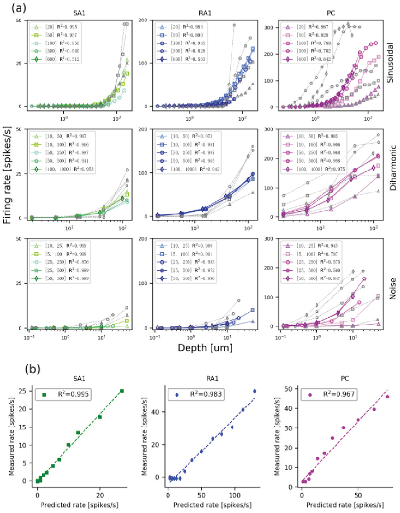
Our model was fit using sinusoidal data from Muniak et al [7]. We first ask whether the units in our model generalize to other vibration stimuli used in that study. This includes sinusoidal, diharmonic and band pass noise stimulation (probe diameter: 1 mm) at different frequencies and different depths. To best test our model, we use the same metric of neural activity used in that study: mean firing rate that a unit would be respond as a function of indentation depth [7]. Since the simulated firing rates are identical across repetitions, the simulated mean firing rate of single-unit was calculated as the number of spikes recorded from one tactile afferent over a duration of 1 second.

Figure 5a plots the predicted responses (colored data) and the measured neural responses (gray data) for the three stimuli (rows) and for the three afferent classes (columns). While most of the predicted responses do not appear to mimic the neural responses, the model does a good job of replicating the trends of firing rate changes. This can be seen in Fig 5b, which plots the observed responses against the predicted responses at 20 Hz for each of the afferent units. For frequencies below 300 Hz, the R²s are almost all higher than 0.9 (listed in Fig 5a). Only at the highest frequencies do the R²s start to drop, often because the observed neural data approach zero, yet even then the model explains more than 50% of the variance. The high correlations mean that our model does a good job of predicating the changes in response. Note that neural responses of single afferents vary greatly [7], so the model’s inability to precisely match the mean firing rate of the populations would not hamper any control functions for operations for prosthetic devices.

Fig. 5.

(a) Mean firing rates from the 3 afferent units for the three types of stimuli. Open gray and colored markers correspond to the measured neural data (adapted from ref. [8]) and model outputs respectively. Numbers in square brackets represent frequencies tested in Hz. (b) Relationship between the observed and predicted firing rates from the 3 afferent units for sinusoidal vibration of 20 Hz. Dashed lines denote best fits.

B. Receptive field sizes

A well-known difference across afferent classes is in the size of their receptive field (RF) [28], which is a basic property of single tactile afferents. The receptive field of any unit is not a fixed area but its extent depends on the intensity and the kind of mechanical stimulus used [29]. The next test of our model is to compare the RFs from the two classes of tactile afferents in response to different indentations with published data from the literature [30]. Note that the model was not fit with RF size data, it was just fit based on the response to a vibrating probe over the center of the RF combined with the implemented conductivity of the resistance network.

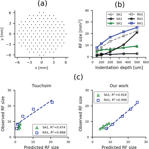
To get an estimate of RF size as a function of indentation depth, we followed the underlying protocol from Vega-Bermudez and Johnson [30]. Specifically, we simulated responses from single-units by orderly indenting a probe (diameter: 0.5 mm) at each location shown in Fig 6a. Individual probes were indented over 200 ms and then withdrawn for 200 ms. Probes were indented 50, 100, 200, 350 and 500 um. RF size was defined as the number of probe positions where the response exceeded 2% of the peak response of that afferent when stimulated at the center of the RF with the same indentation amplitude, divided by the probe density (1.15 probes/mm²). Figure 6b shows the change in RF size as a function of indentation depth for our model (green and blue lines), from Touchsim [13] (black lines) and from the neural data [30] (gray lines). To compare the predicted RF sizes from the models, we plot the observed against the predicted sizes in Fig 6c. The RF sizes from our model were well correlated with the actual RF sizes (R²>0.91, p<0.02); this strong relationship suggests that our resistance network may be a good model of skin mechanics.

Fig. 6.

(a) Probe presentation locations relative to the tactile afferent location. (b) Receptive field size as a function of the relative indentation amplitude for SA1 and RA1 afferents from the current model (green & blue lines), from a recent model (black lines, adapted from [13]) and from the observed data (gray dashed lines, adapted from [30]). (c) Relationship between the observed and predicted RF sizes using the TouchSim model [13] (left panel) and our model (right panel). Dashed lines denote best fits.

C. Responses to dot texture and embossed form

Texture and form perception at the fingertip is a critical component of sensory and motor function in the hand [31]. Here we ask whether single units in our population model can replicate responses to texture and form. In neurophysiological experiments, the single afferent activity has been recorded by repeatedly scanning the texture or form over the single unit, translating the stimulus in a perpendicular direction (typically by about 0.2 mm) between scans. Since the resolution of the resulting spatial event plots (SEPs) depends on the distance of this translation, rather than the space between units, we use the same method to test our model. In an SEP, each small dot represents the occurrence of one action potential. The time of occurrence of each action potential was assigned to a spatial location relative to the stimulus surface by multiplying it by the scanning speed.

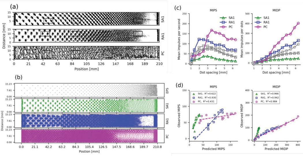
In texture simulation, we first compared our model output to single unit responses (Fig 7a) to embossed dot textures from reference [32]. The dot pattern is shown in the top panel of Fig 7b. Each dot had a diameter of 1 mm and the center-to-center dot spacing decreased linearly from 6.4 to 0.87 mm (from left to right) with the exception of a 10 mm patch at the right, within which the dot spacing remained constant at 0.87 mm. Responses to the whole pattern are shown in the lower panels of Fig 7b, which are equivalent to the SEPs from the single unit data. To summarize the data, we calculated the same two metrics used in the original study [32]. First, we calculated the mean impulses per second (MIPS), by averaging within a window defined by the mean dot-spacing in that region of the pattern. The window extended across the full height of the SEP, but only along the width of the SEP (i.e. the long axis) by an amount equal to three times the local dot spacing. The second metric measured the mean impulses per dot (MIPD), which is calculated as the total number of impulses in the window divided by number of dots in the window.

Fig. 7.

Response to doted texture. (a) Observed SEPs reconstructed from single-unit responses of 3 tactile afferent types by repeatedly scanning the dot pattern across the skin at scanning speed of 60 mm/s and pressing force of 0.6N. From [32], Copyright 1992 Society for Neuroscience. (b) The top panel shows the EPS (probe height 0.5mm). The remaining panels show the stimulated SEPs for the three classes of tactile afferents. (c) Observed (gray, adapted from [32]) and simulated (colored) MIPS and MIPD plotted as a function of dot spacing. (d) Relationship between the observed and predicted MIPS and MIDP.

Fig 7c shows the neural data (gray) and the output from our model (colored lines). With the exception of the PC data, the model does a good job of replicating the responses. This is illustrated in Fig 7d, in which we plot the observed data against the output of the model. We show that the MIPS from the model for both the SA1 and the RA1 were well correlated with the measured data (R² = 0.622 and 0.930, p=2.31×10⁻³ and 4.16×10⁻⁷, respectively). The PC model MIPS outputs were not well correlated with the measured data, but still explains more than 43% of the variance (p=0.020). The model MIPD outputs were even better correlated with the measured data, with all R² values greater than 0.94 (p<1.6×10⁻⁷). These data show that a model fitted only on sinusoidal vibration is able to mimic response to dot textures exceedingly well.

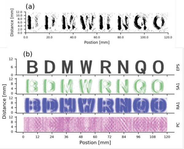
For form simulation, we simulated tactile afferent responses to scanned embossed letters [33]. We selected 4 pairs of letters B-D, M-W, R-N, and Q-O, in which the first letter is commonly perceived as the second letter. As with the texture analysis, we tested these data using a single unit approach creating SEPs as the stimulus was moved along the input array. As illustrated in Fig 8, we also observe letter similarity in the SEPs of our simulated SA1s, which look very similar to the raw data. The SEPs of our simulated RA1s and PCs looked very similar to the raw data (from Figure 2 in reference [34]). In all simulations of scanning the texture and form spatial representations carried by SA1 units are sharper than those carried by RA1 units, while PC responses are insensitive to the spatial structure of the stimulus, which is consistent with results from previous neurophysiological experiments [35].

Fig. 8.

Response to embossed letters. (a) Observed SEPs reconstructed from single SA1 units evoked by repeatedly scanning the letter with shift distance of 0.2 mm at the velocity of 20 mm/s and pressing force of 0.35 N (adapted from [33]). (b) Simulated SEPs reconstructed from single units of the 3 afferent types. The top panel shows the EPS (probe height 1.0 mm).

D. Responses to static shape

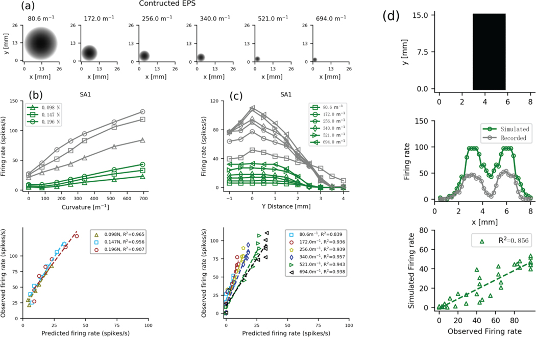
All the simulations above and previous modeling studies [7, 32, 36] have dealt with dynamic stimuli, such as texture or vibrating probes, but a major part of tactile perception deals with shape, which is predominantly encoded during static grasping. Here we present a simulation dealing with static responses to spherical surfaces with different curvatures based on refs [37, 38], and to a 3-mm bar based on ref [39].

The spherical surfaces, with radii ranging from 1.44 mm (694.0 m⁻¹) to 12.4 mm (80.6 m⁻¹), were constructed using multiple probes as shown in Fig 9a. Given that SA1 afferents are thought to encode shape [3, 37, 40], we focus only on this class of tactile afferent. We first simulate how the firing rate of these afferents changes with the stimulus applied directly over the tactile afferent under 3 different pressing forces (Fig. 9b). As is clear from the upper panel, the output of our model has a different firing rate than the mean response of the actual afferents, but, as noted above, this is not surprising as the model output is a single value and individual afferents in the human [38] and non-human primate [37] have a range of sensitives. What matters is the tight correlation shown in the lower panel (all R²>0.90, and p<1.4×10⁻⁴), showing that the model output, which was trained on a vibrating probe, has the same response function to a static shaped stimulus as the measured responses. Similarly, as we move the center of the spherical surface from the center of the simulated tactile afferent, in steps of 0.5 mm with a force of 0.15N, the shape continues to be encoded in the response (Fig 9c). Across the 6 curved surfaces, R²s ranged from 0.839 to 0.957 (all ps<7.4×10⁻⁵), showing that the model does an excellent job of recreating the afferent responses as a function of shape. Thus, the resistance network and the simulated SA1 tactile afferents are able to mimic shape responses to static stimuli, even when the stimuli are placed remote to the RF center and even though the model was fit with responses to vibrating probes.

Fig. 9.

SA1 responses to surface curvature. (a) The EPS to emulate spherical surface with different curvature. (b) Upper panel shows the recorded (gray, adapted from [37]) and simulated (colored) firing rates as function of the curvature for SA1 afferents under different forces. Lower panel shows the relationship between the two for each force. (c) Upper panel shows the firing responses of single SA1 afferents (gray adapted from [37]) and simulated SAI units (green) to the seven curvatures as a function of distance from the tactile afferent center. Lower panel shows the relationship between the two for each curvature. (d) Upper panel shows the EPA to emulate the 3-mm bar. Middle panel show firing rates during the static phase of the response for observed (gray) and simulated (green) SA1 afferents as function of the location with respect to bar stimuli. Lower panel shows the relationship between the observed and simulated and firing rate.

A well-known property of SA1 afferent responses is edge enhancement [41]. This is best seen when a flat stimulus with defined edges (such as in Fig 9d, upper panel) is indented into the skin: responses to the edges are enhanced compared to the response of the plateau (gray data in Fig 9d, middle panel), even though the indentation depth is the same. In order to test this, we used the same strategy as in ref [41]. We created a 3 mm wide, 8 mm height, and 15 mm long bar as illustrated in Fig. 9d upper. The bar was indented into the skin to a depth of 1 mm for 1000 ms (rise and fall time equaled 50 ms). The firing rate was calculated from the static phase of the response (600–950 ms) and compared to the observed response recorded in the same window. The bar was repeatedly indented moving in steps of 0.2 mm parallel with the width of the bar across a total distance of 8 mm, such that the bar started well away from the RF center, moved across it and ended away from it. As illustrated in the green data in the middle plot of Fig 9d, the edges of the bar evoked a higher firing rate for the simulated afferents in a manner similar to that of the actual data, albeit with a different gain. The bottom plot of Fig 9d shows the predicted firing rates as a function of the observed firing rates. Although the predicted responses were correlated with the actual firing rates (R²=0.856, and p=1.43×10⁻¹⁷), they were not as well correlated as for the curved stimuli. This is likely because our simplified model of skin mechanics does not perfectly mimic the complexities of glabrous skin.

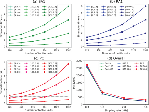
IV. Computation efficiency evaluation

To evaluate the computational efficiency of simulating massive numbers of tactile afferents, we present the maximum number of tactile afferents that allow real-time simulation (MNTARS, as defined in [9]) at different sampling rates for each afferent type. We first show the simulation time as a function of the number of tactile afferents (x-axis), number of probe stimuli and sampling rate for the SA1 (Fig 10a), RA1 (Fig 10b) and PC (Fig 10c) tactile afferents. MNTARS (Fig 10d) was then calculated from the x value at the point where each curve crosses the line of y=1, i.e. where the simulation time takes 1 s. The code of evaluating computation efficiency runs under the condition of keeping about 60% of the physical memory free. Independent of probe number, the current model runs in real time with about 2700 units at a sampling rate of 0.3 kHz, at 1 kHz can handle about 900 units and at 3 kHz can handle about 400 units.

Fig. 10.

Evaluation of computation efficiency. (a), (b), (c) Simulation time is plotted as a function of the number of tactile afferents and as a function of the number of probe stimuli (9, 100, 400) and the sampling rate (0.3, 1, 2 or 3 Hz) for simulating each afferent type. The number of tactile afferents was adjusted by changing density (d) MNTARS changing with sampling rates under different numbers of probe stimuli for each type.

V. Discussion

In the present work, we have simulated the responses of a large cutaneous afferent population and have tested our model on a range of afferent responses as they were recorded from the periphery. Although the model was only fit using a subset of data from probe vibration, it did an excellent job of reproducing responses to texture, a wide range of probe vibrations and statically presented shapes. In addition, it produced relatively realistic receptive field sizes. This suggests that our model does a good job of simulating the neural and mechanical processes going on in the periphery. It also suggests that most properties that influence tactile perception are driven by the basic properties of the end organs in the skin: if this were not true, then features such as shape or receptive field size would not be modeled well by a simulation fit only based on the temporal response properties of vibration data.

A. Comparison with previous work

There are several models attempting to replicate tactile afferent responses in the literature. Among these, the model designed by saal et al may be the most systematic one: it successfully reproduced many properties of single units and population responses [13]. The work of [8] may be most precise model to replicate the evoked action potential of PC afferent, but is limited to just that class of afferent.

Afferent branching is not implemented in previous models and while we did not model it here, we incorporated the idea of branching by covering a certain area for each tactile afferent and connecting tactile afferents using resistance network. This gives us the potential to simulate the afferent population response of the whole hand. In addition, the current work can be implemented as a biomimetic model in electronic skin, as the model adopted in the neuro-inspired e-skin [42], to convert signals of pressure sensor array into biologically accurate tactile responses. A drawback of this approach is that our resistance network must be a symmetrical grid, so the resolution of the system is limited by the grid, and not by the size or arrangement of probes in the EPA.

The model in [12] and TouchSim [13] allows resolution to be set arbitrarily, but requires an iterative operation to compute skin deformation. The benefits of this approach are that it can more accurately mimic skin mechanics and provides more biologically realistic spike timing. The down side is that as stimuli get more complex, the models slow down. By moving to a simplified model of skin mechanics, we were able to run in real time with about 2700 units at a sampling rate of 300 Hz in Python on a laptop independent of stimulus complexity. Indeed, the computational efficiency of our model did not decrease as the number of probe stimuli increased (Fig 10). Nonetheless, the computational efficiency of our model could be further improved by decreasing the density of tactile afferents and /or increasing the diameter of the basic probe.

An additional benefit of our model is that it is relatively easy to fit the all the free parameters using only single-unit responses to vibrating probes. After we have run the fitting code once, we can copy the fitted parameters to the full network.

All of our tests of the model simulated a single-unit by repeatedly exploring (pressing or scanning) the stimulus at or near the center of the tactile afferent. However, the model allows us to record the responses of entire populations of afferents to multiple stimuli and recreate response properties of dot textures, embossed letters, static shapes and other more complex textures and shapes with a single presentation. Running such tests on this model will open up a window into understanding how peripheral afferent populations encode stimuli. Perhaps the most important benefit of the model described here is that the circuit network consisted of resistor elements, which has the potential of being built on a real integrated circuit. such a circuit would further enhance the model’s ability to simulation large populations of afferents in real time.

B. Applications

Having an efficient and accurate mathematical model to quantitatively simulate tactile afferents is useful in many ways. From a basic science standpoint, the proposed model can be a powerful tool to investigate the sense of touch. Recording responses of human or monkey afferents is technically challenging and only yields responses from a single afferent at a time. Even multi-electrode arrays only yield responses from a sparse sample of afferents [43], or the aggregate activity of a large number of fibers [44, 45].

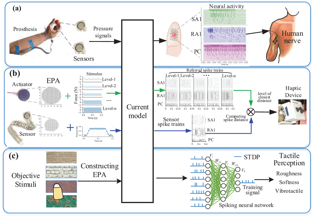
There are also many practical implementations. As illustrated in Fig 11a, an exciting use of this model is in brain-machine interfaces such as prosthesis. Like the Touchsim model adopted in a recent prosthetic application [46], this model can also be used to converted signals detected by sensors installed on the prosthetic hand into desired patterns of action potentials, which can then be implemented in the peripheral nerve of amputated patients to restore natural sensation of touch when contacting with an object.

Fig. 11.

Schematic diagram of controlling haptic device and prosthesis and modelling tactile perception using current model.

Another application of the current model is in haptic devices which provide remote human operators (such as in robot-assisted surgery [47, 48]) with a sense of touch. Despite extensive research done in the field of haptics, current feedback technologies are far from replicating the natural sense of touch. Implementing a model that can control haptic feedback, by rapidly reproducing an afferent population response, benefits the efficiency of presenting natural feedback for haptic devices. As illustrated in Fig. 11b, we can set several stimulus levels for each actuator and record the population spiking trains for each level. Then each actuator was controlled with stimulus level whose spiking train is most approximate to the output spiking trains evoked by sensor signals.

As shown in Fig. 11c, the model of afferent population responses also provides a valuable tool to investigate tactile perception properties such as roughness, and softness or vibration intensity in response to different stimuli. Neurophysiological studies have shown that the relation between our perceptions of these properties and population responses of the 3 tactile afferents is clear. For instance, afferent responses are even better predictors of perceived roughness accounting for 95% of the variance than is vibratory power [5]. Perceived vibration intensity is perfectly predicted by the weighted firing rate evoked in afferents located under or near the locus of stimulation of 3 afferent types [7]. This work also lays the foundation to implement spiking neural network of deep learning algorithm for predicting tactile perception as shown in Fig 11c.

A frequently forgotten role of RA1 afferents is in the fine control of precision grip force: local slips on the finger pad generate a slight increase in grip force [49]. An accurate model of RA1 afferents, as in our model, would thus enable the automatic correction of precision grip force in robots with haptic feedback implemented in this way.

C. Limitations

In this study, we present a simplified model to recreate key properties of an afferent population response with the aim of being able to simulate the responses of large numbers of afferents in real time. As noted above, there are significant trade-offs that we have made to allow for this high processing speed. First, our model has a symmetrical grid and does not have the flexibility to mimic the actual arrangement of afferent RFs on the skin. Second, while the spike timing from our model is precise when tested with oscillating stimuli [9], the spiking is not biologically realistic. As such, we have analyzed responses in terms of mean firing rate. We think this is a reasonable trade off as many peripheral nerve recording studies use mean firing rate as a metric, particularly for stimuli that do not move across the skin. And while it is likely that spike timing precision is critical for dynamic stimuli [50], our previous work shows similar phase locking to recorded responses [9].

Our model also shares similar limitations with other state-of-the-art tactile models. We chose to only simulate responses for SA1, RA, and PC afferents. Given that SA2 afferents, since they lack a clear response profile to vibrating stimuli, are predominantly responsive to stretch and are not present in non-human primate glabrous skin, where most of the data in the field has been recorded [16]. In addition, our model does not take into account the curvature of the skin, however our EPA system supports simulating more complex stimuli in 3D coordinates while working within a two dimensional matrix. As such, we could potentially incorporate the curvature of the skin by these means. However, it is unclear whether the resulting outputs would accurately mimic responses of afferents on the side of the finger [51]. Finally, like previous models, ours was also limited to solid stimuli indenting directly into the skin.

VI. Conclusion

The present work describes a model, which combines a skin contact model, a resistance network model and single unit models to rapidly reproduce the responses of large numbers of mechanoreceptive afferents. The model was fit with a simple vibrating probe stimulus placed over the tactile afferent, but reproduces receptive field size and responses to texture, embossed letters and statically presented shaped stimuli. Our model may provide ways to control advanced neuroprostheses and robots and can be implemented to enhance the realism of haptic displays of virtual tactile stimuli, or to design highly realistic prostheses with tactile feedback.

References

- [1].Delhaye BP, Long KH and Bensmaia SJ, “Neural basis of touch and proprioception in primate cortex,” Compr. Physiol, vol. 8, pp. 1575–1602, 2018. [DOI] [PMC free article] [PubMed] [Google Scholar]
- [2].Suresh AK, Saal HP and Bensmaia SJ, “Edge orientation signals in tactile afferents of macaques,” J. Neurophysiol, vol. 116, pp. 2647–2655, 2016. [DOI] [PMC free article] [PubMed] [Google Scholar]
- [3].Khalsa PS et al. , “Encoding of shape and orientation of objects indented into the monkey fingerpad by populations of slowly and rapidly adapting mechanoreceptors,” J. Neurophysiol, vol. 79, pp. 3238–3251, 1998. [DOI] [PubMed] [Google Scholar]
- [4].Hollins M. and Bensmaia SJ, “The coding of roughness,” Can. J. Exp. Psychol, vol. 61, pp. 184–195, 2007. [DOI] [PubMed] [Google Scholar]
- [5].Weber AI et al. , “Spatial and temporal codes mediate the tactile perception of natural textures,” Proc. Natl. Acad. Sci. U.S.A, vol. 110, pp. 17107–17112, 2013. [DOI] [PMC free article] [PubMed] [Google Scholar]
- [6].Hsiao SS, Lane J. and Fitzgerald P, “Representation of orientation in the somatosensory system,” Behav. Brain Res, vol. 135, pp. 93–103, 2002. [DOI] [PubMed] [Google Scholar]
- [7].Muniak MA et al. , “The neural coding of stimulus intensity: linking the population response of mechanoreceptive afferents with psychophysical behavior,” J. Neurosci, vol. 27, pp. 11687–11699, 2007. [DOI] [PMC free article] [PubMed] [Google Scholar]
- [8].Biswas A, Manivannan M. and Srinivasan MA, “Vibrotactile sensitivity threshold: Nonlinear stochastic mechanotransduction model of the Pacinian corpuscle,” IEEE Trans. Haptics, vol. 8, pp. 102–113, 2015. [DOI] [PubMed] [Google Scholar]
- [9].Ouyang Q. et al. “A Python code for simulating single tactile receptors and the spiking responses of their afferents,” Front. Neuroinform, vol. 13, pp. 27, 2019. [DOI] [PMC free article] [PubMed] [Google Scholar]
- [10].Maeno T, Kobayashi K. and Yamazaki N, “Relationship between the structure of human finger tissue and the location of tactile receptors,” JSMEInt. J. C. Mech. Sy, vol. 41, pp. 94–100, 1998. [Google Scholar]
- [11].Dandekar K, Raju BI and Srinivasan MA, “3-D finite-element models of human and monkey fingertips to investigate the mechanics of tactile sense,” J. Biomech. Eng, vol. 125, pp. 682–691, 2003. [DOI] [PubMed] [Google Scholar]
- [12].Sripati AP, Bensmaia SJ and Johnson KO, “A continuum mechanical model of mechanoreceptive afferent responses to indented spatial patterns,” J. Neurophysiol, vol. 95, pp. 3852–3864, 2006. [DOI] [PMC free article] [PubMed] [Google Scholar]
- [13].Saal HP et al. , “Simulating tactile signals from the whole hand with millisecond precision,” Proc. Natl. Acad. Sci. U.S.A, vol. 114, pp. E5693–E5702, 2017. [DOI] [PMC free article] [PubMed] [Google Scholar]
- [14].Dong Y. et al. , “A simple model of mechanotransduction in primate glabrous skin,” J. Neurophysiol, vol. 109, pp. 1350–1359, 2013. [DOI] [PMC free article] [PubMed] [Google Scholar]
- [15].Gerling GJ et al. “Validating a population model of tactile mechanotransduction of slowly adapting type I afferents at levels of skin mechanics, single-unit response and psychophysics,” IEEE Tran. Haptics, vol. 7, pp. 216–228, 2014. [DOI] [PMC free article] [PubMed] [Google Scholar]
- [16].Pare M, Smith AM and Rice FL, “Distribution and terminal arborizations of cutaneous mechanoreceptors in the glabrous finger pads of the monkey,” J. Comp. Neurol, vol. 445, pp. 347–359, 2002. [DOI] [PubMed] [Google Scholar]
- [17].Pruszynski JA and Johansson RS, “Edge-orientation processing in first-order tactile neurons,” Nat. Neurosci, vol. 17, pp. 1404–1409, 2014. [DOI] [PubMed] [Google Scholar]
- [18].Johansson RS and Vallbo AB, “Tactile sensibility in the human hand: relative and absolute densities of four types of mechanoreceptive units in glabrous skin,” J. Physiol, vol. 286, pp. 283–300, 1979. [DOI] [PMC free article] [PubMed] [Google Scholar]
- [19].Mountcastle VB, Talbot WH and Kornhuber HH, The Neural Transformation of Mechanical Stimuli Delivered to the Monkey’s Hand: John Wiley & Sons, Ltd., 1966. [Google Scholar]
- [20].Hodgkin AL and Huxley AF, “A quantitative description of membrane current and its application to conduction and excitation in nerve,” J. Physiol, vol. 117, pp. 500–544, 1952. [DOI] [PMC free article] [PubMed] [Google Scholar]
- [21].Tsumoto K. et al. , “Bifurcations in Morris-Lecar neuron model,” Neurocomputing, vol. 69, pp. 293–316, 2006. [Google Scholar]
- [22].FitzHugh R, “Impulses and physiological states in theoretical models of nerve membrane,” Biophys. J, vol. 1, pp. 445–466, 1961. [DOI] [PMC free article] [PubMed] [Google Scholar]
- [23].Becker WM, Kleinsmith LJ and Bertoni GP, “Signal transduction mechanisms: I. Electrical and synaptic signaling in neurons,” in The world of the cell: Benjamin Cummings, San Francisco, 2009. [Google Scholar]
- [24].Bensmaia S. et al. , “Conveying tactile feedback using a model of mechanotransduction,” in IEEE Biomedical Circuits and Systems Conference, 2008, pp. 137–140. [DOI] [PMC free article] [PubMed] [Google Scholar]
- [25].Tal D. and Schwartz EL, “Computing with the leaky integrate-and-fire neuron: logarithmic computation and multiplication,” Neural Comput, vol. 9, pp. 305–318, 1997. [DOI] [PubMed] [Google Scholar]
- [26].Bolanowski SJ Jr et al. , “Four channels mediate the mechanical aspects of touch,” J. Acoust. Soc. Am, vol. 84, pp. 1680–94, 1988. [DOI] [PubMed] [Google Scholar]
- [27].Johnson KO, Yoshioka T. and Vega-Bermudez F, “Tactile functions of mechanoreceptive afferents innervating the hand,” J. Clin. Neurophysiol, vol. 17, pp. 539, 2000. [DOI] [PubMed] [Google Scholar]
- [28].Johansson RS, “Tactile sensibility in the human hand: receptive field characteristics of mechanoreceptive units in the glabrous skin area,” J. Physiol, vol. 281, pp. 101, 1978. [DOI] [PMC free article] [PubMed] [Google Scholar]
- [29].Vallbo AB and Johansson RS, “Properties of cutaneous mechanoreceptors in the human hand related to touch sensation,” Hum. Neurobiol, vol. 3, pp. 3–14, 1984. [PubMed] [Google Scholar]
- [30].Vega-Bermudez F. and Johnson KO, “SA1 and RA receptive fields, response variability, and population responses mapped with a probe array,” J. Neurophysiol, vol. 81, pp. 2701, 1999. [DOI] [PubMed] [Google Scholar]
- [31].Johnson KO and Hsiao SS, “Neural mechanisms of tactual form and texture perception,” Ann. Rev. Neurosci, vol. 15, pp. 227–250, 1992. [DOI] [PubMed] [Google Scholar]
- [32].Phillips JR, Johansson RS and Johnson KO, “Responses of human mechanoreceptive afferents to embossed dot arrays scanned across fingerpad skin,” J. Neurosci, vol. 12, pp. 827–39, 1992. [DOI] [PMC free article] [PubMed] [Google Scholar]
- [33].Vega-Bermudez F, Johnson KO and Hsiao SS, “Human tactile pattern recognition: active versus passive touch, velocity effects, and patterns of confusion,” J. Neurophysiol, vol. 65, pp. 531–546, 1991. [DOI] [PubMed] [Google Scholar]
- [34].Phillips JR, Johnson KO and Hsiao SS, “Spatial pattern representation and transformation in monkey somatosensory cortex,” Proc. Natl. Acad. Sci. U.S.A, vol. 85, pp. 1317–21, 1988. [DOI] [PMC free article] [PubMed] [Google Scholar]
- [35].Yoshioka T. et al. , “Neural coding mechanisms underlying perceived roughness of finely textured surfaces,” J. Neurosci, vol. 21, pp. 6905–6916, 2001. [DOI] [PMC free article] [PubMed] [Google Scholar]
- [36].Phillips JR, Johansson RS and Johnson KO, “Representation of braille characters in human nerve fibres,” Exp. Brain. Res, vol. 81, pp. 589–92, 1990. [DOI] [PubMed] [Google Scholar]
- [37].Goodwin AW, Browning AS and Wheat HE, “Representation of curved surfaces in responses of mechanoreceptive afferent fibers innervating the monkey’s fingerpad,” J. Neurosci, vol. 15, pp. 798–810, 1995. [DOI] [PMC free article] [PubMed] [Google Scholar]
- [38].Goodwin AW, Macefield VG and Bisley JW, “Encoding of object curvature by tactile afferents from human fingers,” J. Neurophysiol, vol. 78, pp. 2881–2888, 1997. [DOI] [PubMed] [Google Scholar]
- [39].Johnson KO and Phillips JR, “Tactile spatial resolution. I. Two-point discrimination, gap detection, grating resolution, and letter recognition,” J. Neurophysiol, vol. 46, pp. 1177–1192, 1981. [DOI] [PubMed] [Google Scholar]
- [40].Dodson MJ et al. , “Peripheral neural mechanisms determining the orientation of cylinders grasped by the digits,” J. Neurosci, vol. 18, pp. 521–530, 1998. [DOI] [PMC free article] [PubMed] [Google Scholar]
- [41].Phillips JR and Johnson KO, “Tactile spatial resolution. II. Neural representation of bars, edges, and gratings in monkey primary afferents,” J. Neurophysiol vol. 46, pp. 1192–1203, 1981. [DOI] [PubMed] [Google Scholar]
- [42].Lee WW et al. , “A neuro-inspired artificial peripheral nervous system for scalable electronic skins,” Sci. Robotics, vol. 4, pp. eaax2198, 2019. [DOI] [PubMed] [Google Scholar]
- [43].Clark GA et al. , “Recording sensory and motor information from peripheral nerves with Utah Slanted Electrode Arrays,” in Proc. 2011 Annual International Conference of the IEEE Engineering in Medicine and Biology Society, 2011, pp. 4641–4644. [DOI] [PubMed] [Google Scholar]
- [44].Haugland MK, Hoffer JA and Sinkjaer T, “Skin contact force information in sensory nerve signals recorded by implanted cuff electrodes,” IEEE Trans. Rehabil. Eng, vol. 2, pp. 18–28, 2002. [Google Scholar]
- [45].Yoo PB and Durand DM, “Selective recording of the canine hypoglossal nerve using a multicontact flat interface nerve electrode,” IEEE Trans. Biomed. Eng, vol. 52, pp. 1461–1469, 2005. [DOI] [PubMed] [Google Scholar]
- [46].George JA et al. , “Biomimetic sensory feedback through peripheral nerve stimulation improves dexterous use of a bionic hand,” Sci. Robotics, vol. 4, pp. eaax2352, 2019. [DOI] [PubMed] [Google Scholar]
- [47].Abiri A. et al. , “Artificial palpation in robotic surgery using haptic feedback,” Surg. Endosc, vol. 33, pp. 1252–1259, 2019. [DOI] [PMC free article] [PubMed] [Google Scholar]
- [48].Abiri A. et al. , “Suture Breakage Warning System for Robotic Surgery,” IEEE Trans. Biomed. Eng, vol. 66, pp. 1165–1171, 2019. [DOI] [PMC free article] [PubMed] [Google Scholar]
- [49].Macefield VG, Hager-Ross C. and Johansson RS, “Control of grip force during restraint of an object held between finger and thumb: responses of cutaneous afferents from the digits,” Exp. Brain Res, vol. 108, pp. 155–171, 1996. [DOI] [PubMed] [Google Scholar]
- [50].Harvey MA et al. , “Multiplexing Stimulus Information through Rate and Temporal Codes in Primate Somatosensory Cortex,” PLOS Biol, vol. 11, pp. e1001558, 2013. [DOI] [PMC free article] [PubMed] [Google Scholar]
- [51].Bisley JW, Goodwin AW and Wheat HE, “Slowly adapting type I afferents from the sides and end of the finger respond to stimuli on the center of the fingerpad,” J. Neurophysiol, vol. 84, pp. 57–64, 2000. [DOI] [PubMed] [Google Scholar]
Associated Data
This section collects any data citations, data availability statements, or supplementary materials included in this article.