Disease momentum: Estimating the reproduction number in the presence of superspreading

Abstract

A primary quantity of interest in the study of infectious diseases is the average number of new infections that an infected person produces. This so-called reproduction number has significant implications for the disease progression. There has been increasing literature suggesting that superspreading, the significant variability in number of new infections caused by individuals, plays an important role in the spread of SARS-CoV-2. In this paper, we consider the effect that such superspreading has on the estimation of the reproduction number and subsequent estimates of future cases. Accordingly, we employ a simple extension to models currently used in the literature to estimate the reproduction number and present a case-study of the progression of COVID-19 in Austria. Our models demonstrate that the estimation uncertainty of the reproduction number increases with superspreading and that this improves the performance of prediction intervals. Of independent interest is the derivation of a transparent formula that connects the extent of superspreading to the width of credible intervals for the reproduction number. This serves as a valuable heuristic for understanding the uncertainty surrounding diseases with superspreading.

1. Introduction

The reproduction number, R_t ≡ R, gives the average number of new infections caused by a single infected person throughout the infectious period. In contrast to the basic reproduction number R₀, which describes the reproduction of the virus in a naïve, unmitigated population, R (sometimes called the effective reproduction number) varies through time as the epidemic develops and the opportunities for transmission change due to, for example, behavioral response, seasonality, and changes in the relative size of the susceptible population. In every population, some individuals will cause considerably more infections than others - a phenomenon known as superspreading. It can be quantified using a framework provided by Lloyd-Smith et al. (Lloyd-Smith et al., 2005). In this paper, we extend the model of Cori et al. (Cori et al., 2013) to include the phenomenon of superspreading. Our goal is to better quantify the uncertainty inherent in this type of estimate of R, not to derive a more accurate estimate.

Ultimately we are interested in the estimation of R and specifically the question whether, given current case numbers, we can claim with statistical guarantees that R ≤ 1 or R > 1. Given the growing body of evidence about the existence and importance of superspreaders (Adam et al., 2020; Liu et al., 2020), we incorporate this feature into our models. We observe two important effects: first, it becomes increasingly difficult to accurately estimate the reproduction number R in the presence of superspreading; second, models with superspreading produce prediction intervals for new cases that have improved coverage compared to those without superpreading. Both of these are demonstrated in our Austrian case-study in Section 3. In particular, it becomes infeasible even in early May to support the claim that R < 1 using our methods. This is a critical period of time as it coincides with the removal of lockdown restrictions in Austria.

In particular, the width of a credible interval for R should decrease as a function of total number of cases used during estimation and increase with the extent of superspreading. Let S be the set of days used to estimate R in the nowcasting framework presented in Section 1.1 and assume that the (average) reproduction number does not change over time. One would then expect that a (1 − α)% credible interval to have width approximately equal to

$$\frac{2z_{1-\alpha /2}}{\sqrt{k\sum _{s\in S}{I}_s}},$$ (1.1)

where z_1−α/2 is the (1 − α/2) quantile of the standard normal distribution and for values of dispersion parameter k much smaller than 1, which corresponds to scenarios with high superspreading. We derive this exact functional form in a simplified model introduced in Section 2.2.

1.1. Nowcasting

The goal of nowcasting is to get accurate estimates of the current state of an epidemic. Given that our observed infections are random observations from an underlying process, our goal is to understand the parameters of that process, particularly with respect to the reproduction number. In addition, we define a time-varying parameter we call the “momentum” of an epidemic, which is a random realization of population infectiousness at a time-point which accounts for superspreading. This is introduced formally in Section 2.1.

Benchmark methods for estimating the reproduction number R include those of Cori et al. (Cori et al., 2013) and Wallinga and Teunis (Wallinga & Teunis, 2004). The method of Cori et al. (Cori et al., 2013) provides near real-time estimation of R and is implemented in the R software package ‘EpiEstim’. An improvement of this framework is given in Thompson et al. (Thompson et al., 2019) which accounts for variability in the generation interval (defined below). A substantial extension of the EpiEstim-package (‘EpiNow’) was developed by a group of researchers at the London School of Hygiene and Tropical Medicine (Abbott et al., 2020). The method of Wallinga and Teunis (Wallinga & Teunis, 2004) provides an alternate estimate for historical values of R. Contrary to the methods discussed in this paper, it requires observations from both before and after the time point at which an estimate for R is desired. An important overview of other estimation methods and challenges due to COVID-19 is given in Gostic et al. (Gostic et al., 2020) and a comparative analysis of statistical methods to estimate R is given in O’Driscoll et al. (O’Driscoll et al., 2020). If the epidemic is at an early stage, the reproduction number R and the rate of exponential growth are connected by the Euler-Lotka equation (Ma, 2020; Wallinga & Lipsitch, 2007).

As we follow the framework of Cori et al. (Cori et al., 2013), we briefly describe their basic model. Let I₀ be the number of initial infections and I₁, I₂, …be the number of new infections on days 1, 2, …. By ${\left(w_n\right)}_{n\ge 1}$ we denote the generation interval distribution. If J_m denotes the number of people infected by a specific person on the m-th day after this person got infected, then we have for $m\in \mathbb{N}$

$$w_m=\frac{\mathbb{E}\left[J_m\right]}{{\sum }_{l=1}^{\infty }\mathbb{E}\left[J_l\right]}.$$

We assume that a newly infected individual does not cause secondary cases on the same day, corresponding to w₀ = 0. The generation interval can be interpreted as the infectiousness profile of infected persons.

The basic model of Cori et al. (Cori et al., 2013) assumes that the stochastic process of total new infections on day t, ${\left(I_t\right)}_{t\in \mathbb{N}}$, satisfies

$$I_t~\text{Poisson}\left(R_t\sum _{m=1}^t{I}_{t-m}{w}_m\right),$$ (1.2)

for a sequence of numbers $R_t,t\in \mathbb{N}$. In practice it is often assumed that the generation interval distribution is given as a Gamma distribution that has been discretized in such a way that w_m = 0 for all m larger than some cut-off number ν (Gostic et al., 2020). As a result, the sum in (1.2) will only have $\nu \in \mathbb{N}$ summands, and to make assertions about I_t we only have to consider the case numbers I_t−ν, …, I_t−1. As ν is a parameter that can vary between diseases, this term is kept and used throughout our model description in Section 2.1.

When estimating the time-varying reproduction number, Cori et al. (Cori et al., 2013) assume that the reproduction number has stayed constant over a window of τ days. In this case, for s ∈ (t − τ + 1, …, t), equation (1.2) simplifies to

$$I_s~\text{Poisson}\left(R\sum _{m=1}^{\nu }{I}_{s-m}{w}_m\right).$$ (1.3)

In order to treat R as fixed in the above expression, it is necessary to only explicitly model a subset of time points, lest R be assumed constant over all time points.

Note that the reproduction number in the sense of (1.3) does not denote the number of people that actually have been infected by a given individual, but rather describes what one would expect in an “average” evolution of the epidemic. Furthermore, while R = R_t is assumed to be constant over the window of width τ, as this window moves through time the method produces estimates of R that slowly vary over time.

1.2. Heterogeneity in reproduction numbers

The motivation for our hierarchical Bayesian approach follows the framework of superspreading provided in Lloyd-Smith et al. (Lloyd-Smith et al., 2005). Even if the reproduction number R is constant over a small window of time, it might vary between individuals. We consider the reproduction number of a specific person with index x to be drawn randomly as

$$r_x~\text{Gamma}\left(k,\text{rate}=k/R\right).$$ (1.4)

This distribution has mean R and variance R²/k. Note that the above gamma distribution will also be referred to as having dispersion parameter k. The degenerate case k = ∞ corresponds to the deterministic case where r_x = R for all individuals and leads to the model in (1.3). Given r_x = r, this person causes Poisson(r) new infections. If one integrates out the Poisson parameter r, one is left with the unconditional number of descendants which follows a negative binomial distribution with mean R and variance R + R²/k. This negative binomial model is further analyzed in Section 2.2.

A basic extension of (1.3) that follows the concept of random individual reproduction numbers in the sense of Lloyd-Smith et al. (Lloyd-Smith et al., 2005) is to assign, on day t, the individual reproduction numbers $r_1^t,\dots ,r_{I_t}^t$ to the I_t individuals that got infected on this day. This leads to the recursion

$$I_t~\text{Poisson}\left(\sum _{m=1}^{\nu }{w}_m\sum _{x=1}^{I_{t-m}}{r}_x^{t-m}\right),$$ (1.5)

where the individual reproduction numbers $r_x^m$ are drawn i.i.d. according to (1.4). Note that for the degenerate case k = ∞, (1.5) recovers (1.3). This forms the foundation of the model explained in detail in Section 2.1.

The theme of the present paper is close to that of Donnat and Holmes (Donnat & Holmes, 2020), in which heterogeneity in R between groups is explicitly modeled. While the high-level descriptions of these models sound nearly identical, those models are relevantly different than ours. In particular, Donnat and Holmes (Donnat & Holmes, 2020) are interested in estimating group-specific or time-varying reproduction numbers for different geographical regions and age groups. On one hand, with sufficient group-specific data, this provides tools of a much broader scope than we present here; on the other hand, it is assumed that within-group variability is negligibly small. Instead, we focus on aggregate data from a single geographical region but do not assume that individual variability is negligible. Rather, this is precisely the variability we are interested in modeling. Furthermore, our critiques of the estim ability of the reproduction number transfers to their setting as well: if within-group variability exists, group-specific reproduction numbers are more difficult to estimate than previously acknowledged.

2. Methods

This section introduces two methods. First, the “momentum” model formulates the estimation problem as a Bayesian Poisson regression. Second, the “generation” model is a simplification which provides a fast approximation to the momentum model as well as an explicit formula for dependence of credible interval width on k. Both are of interest beyond COVID modeling and aim to address different goals: precise estimation (momentum) and valuable speed and heuristics (generation).

2.1. The “Momentum” model

As mentioned in the introduction, we identify an unobserved random variable which we term the “momentum” of the epidemic. This follows from a simple notational change in (1.5) according to the observation that a sum of i.i.d. Gamma random variables is also Gamma distributed with the same dispersion parameter. We rewrite (1.5) as

$$I_t~\text{Poisson}\left(\sum _{m=1}^{\nu }{w}_m{\theta }_{t-m}\right),$$ (2.1)

where

$${\theta }_t=\sum _{x=1}^{I_t}{r}_x^t~\text{Gamma}\left(I_{t}k,\text{rate}=k/R\right).$$ (2.2)

The terms ${\left({\theta }_t\right)}_{t\ge 0}$ are collectively referred to as the “momentum” of the disease. They will be treated as a set of nuisance parameters of the offspring distribution, as our primary interest lies in estimating the reproduction number R. In our Bayesian framework introduced below, R is a hyperparameter of the prior distribution for ${\left({\theta }_t\right)}_{t\ge 0}$. Equation (2.1) describes the distribution of I_t conditioned on its whole past, i.e., I_s, θ_s, s < t. Analogously, equation (2.2) describes θ_s given its history. The difference in what we understand as the relative past originates from θ_t being conceptually determined “after” I_t.

For increased clarity of the form of the model and the estimation methods required, we recast our model as a Bayesian Poisson regression using vector notation. This is made painfully explicit by using an arrow as in $\vec{I}$ for vectors. Following Cori et al. (Cori et al., 2013), we estimate R by explicitly modeling a set of τ days over which we assume R to be constant. We specify the regression function for each observation in this estimation window. To condense notation, we use [l], for $l\in \mathbb{N}$, to be the vector (1, 2, …, l). Similarly, [l, m] for $l,m\in \mathbb{N}$ is shorthand for the vector (l, l + 1, …, m), i.e., [l] = [1, l]. This notation will primarily be used for vector indices. Furthermore, the indices of our vectors increase in time. As such, our generation interval truncated to ν days can be condensely written as ${\vec{w}}_{\left[\nu \right]}=\left(w_1,\dots ,w_{\nu }\right)$. Similarly, the τ observations we model are given by ${\vec{I}}_{\left[t-\tau +1,t\right]}=\left(I_{t-\tau +1},\dots ,I_t\right)$.

As a regression model for ${\vec{I}}_{\left[t-\tau +1,t\right]}$, equation (2.1) can be written as

$$\begin{array}{ccc}{\vec{I}}_{\left[t-\tau +1,t\right]}& ~& \text{Poisson}\left(W{\vec{\theta }}_{\left[t-\nu -\tau +1,t-1\right]}\right)\text{where}\end{array}$$ (2.3)

$$\begin{array}{ccc}W& =& \left(\begin{array}{cccccccc}{w}_{\nu }& w_{\nu -1}& \dots & w_1& 0& 0& \cdots & 0\\ 0& w_{\nu }& w_{\nu -1}& \dots & w_1& 0& \cdots & 0\\ ⋮& \ddots & \ddots & \ddots & \ddots & \ddots & \cdots & ⋮\\ 0& \cdots & 0& w_{\nu }& w_{\nu -1}& \dots & w_1& 0\\ 0& \cdots & 0& 0& w_{\nu }& w_{\nu -1}& \dots & w_1\end{array}\right)\end{array}$$

In the above expression, we have a fixed covariate matrix W which is a function of the generation interval w_[ν]. The momentum parameters ${\vec{\theta }}_{\left[t-\nu +\tau -1,t-1\right]}$ are seen to be the regression parameters to be estimated. Note that the expressions in the previous display suppress the notation for conditioning on all observations before time t − τ + 1. Furthermore, given ${\vec{\theta }}_{\left[t-1\right]}$, I_t is independent of ${\vec{I}}_{\left[t-1\right]}$.

We place a prior distribution on $\vec{\theta }$ which depends on R as in equation (2.2), as well as a hyperprior on R to account for the previously identified uncertainty in the distribution of R as reported in Abbott et al. (Abbott et al., 2020). As we have parameterized the gamma prior on θ_t to have mean I_tR, the conjugate hyperprior for R is the inverse-gamma distribution. This is transparent in the posterior distribution given by equation (2.4) below. Hence we use an inverse-gamma hyperprior on R, where these hyperparameters are set to match the results of Abbott et al. (Abbott et al., 2020). As such, we assume that R has mean 2.6 and standard deviation 2, yielding shape parameter 3.69 and rate parameter 6.994:

$$\begin{array}{ccc}R& ~& \text{Inv}-\text{Gamma}(\text{3.69, rate }=\text{ 6.994}).\end{array}$$

An a priori distribution for R is itself uncertain and one could theoretically place additional hyperpriors on the parameters of this inverse-gamma distribution. That being said, the change would increase computational complexity while introducing hyper-hyperparameters that would be difficult to estimate. Hence, this proposal distribution for R is treated as fixed.

This regression formulation is important as it highlights the latent variables $\vec{\theta }$ that are required to fully determine the generative model. It also focuses attention on which observations are conditioned upon and which are treated as random, i.e., the τ observations to which we fit the model are treated as random. This is relevant as more than τ nuisance parameters are present, namely ν + τ − 1. Observe that the earliest data point is I_t−τ+1, which itself requires a history of ν momentum values of $\vec{\theta }$ to determine.

While we also think of individual reproduction numbers as changing over time due to factors such as changes in social restrictions, the assumption of constant R over a period renders this moot. Likewise, we set k to be a constant for the results presented in Section 3, as k is best estimated with contact tracing data instead of case count data. We set k = 0.072, in line with the results of Laxminarayan et al. (Laxminarayan et al., 2020), which estimated the extent of superspreading for COVID-19 from Indian data. This is also within the range of parameter values identified in Endo et al. (Endo et al., 2020).

Alternatively, it is possible to consider an independently estimated distribution for k. To estimate the momentum model with random k, one can merely draw k from a proposal distribution and estimate the momentum model with this fixed value. This process is repeated for many sampled values of k, and the posterior samples for R and I_t from all k are combined. This follows the same methodology as Thompson et al. (Thompson et al., 2019), where the generation interval was estimated with a separate data set before fitting model (1.3) without superspreading. Brief results for this case are presented in Appendix B as none of the results change significantly. The joint estimation of k and R within the momentum model appears infeasible as k is the dispersion parameter of the nuisance parameter distribution. This makes learning about k using this data highly challenging.

A full derivation of the posterior distribution of the pair $R,{\vec{\theta }}_{\left[t\right]}$ given ${\vec{I}}_{\left[t\right]}$ is given in Appendix A. We obtain as posterior

$$\begin{array}{ccc}& & p\left(R,{\vec{\theta }}_{\left[t-\tau -\nu +1,t-1\right]}|{\vec{I}}_{\left[t-\tau -\nu +1,t\right]}\right)\\ & \propto & p\left({\vec{I}}_{\left[t-\tau +1,t\right]},{\vec{\theta }}_{\left[t-\tau +1,t-1\right]}|{\vec{\theta }}_{\left[t-\tau -\nu +1,t-\tau \right]},{\vec{I}}_{\left[t-\tau -\nu +1,t-\tau \right]},R)p({\vec{\theta }}_{\left[t-\tau \right]},R|{\vec{I}}_{\left[t-\tau \right]}\right)\\ & \propto & \left(\prod _{s=t-\tau +1}^t{\left(\sum _{m<s}{w}_{s-m}{\theta }_m\right)}^{I_s}{e}^{-\sum _{m<s}{w}_{s-m}{\theta }_m}\right)\\ & & \cdot \left(\prod _{s=t-\tau +1}^{t-1}\frac{k^{I_{s}k}}{\mathrm{\Gamma }\left(I_{s}k\right)R^{I_{s}k}}{\theta }_s^{I_{s}k-1}{e}^{-\frac{k}{R}{\theta }_s}\right)\left(\prod _{s=t-\nu -\tau +1}^{t-\tau }\frac{k^{I_{s}k}}{\mathrm{\Gamma }\left(I_{s}k\right)R^{I_{s}k}}{\theta }_s^{I_{s}k-1}{e}^{-\frac{k}{R}{\theta }_s}\right)\\ & & \cdot \left(R^{-3.69-1}{e}^{-6.994/R}\right),=.\end{array}$$ (2.4)

The first line of (2.4) specifies the distribution of the observations given all other parameters, and the third line gives the inverse-gamma prior for R. The second line describes the distribution of $\vec{\theta }$, and we have explicitly partitioned the indices into two sets. The values θ_s in the first index set [t − τ + 1, t − 1] require no special discussion as they depend on values I_s which are being explicitly modeled. The values of θ_s in the second index set [t − ν − τ + 1, t − τ], however, treat the corresponding I_s values as fixed and constant. This is done so that we do not need to specify further nuisance parameters before time t − τ − ν + 1. Doing so would create an infinite recursion in historical observations, requiring us to treat R_t as fixed for all t. Hence we need not only a prior for R, but also for ${\vec{\theta }}_{\left[t-\tau -\nu +1,t-\tau \right]}$. More details are provided in Appendix A.

In order to condense notation for summations in exponents, let S be the index set for the second product; i.e., S = {t − ν − τ + 1, t − ν − τ + 2, …, t − 1}. The additional shorthand below drops “s ∈” from s ∈ S. With this notation, the posterior distribution of R given $\vec{\theta }$ and $\vec{I}$ is

$$p\left(R|{\vec{\theta }}_{\left[t-1\right]},{\vec{I}}_{\left[t\right]}\right)\propto R^{-k\sum _S{I}_s-3.69-1}{e}^{\left(-k\sum _S{\theta }_s-6.994\right)R^{-1}},$$

which is Inv-Gamma(k∑_SI_s + 3.69, k∑_Sθ_s + 6.994). A perhaps counter-intuitive observation is that the posterior distribution of R does not depend on the generation interval ${\vec{w}}_{\left[\nu \right]}$. This is the result of conditioning on $\vec{\theta }$ versus integrating it out as done in Lloyd-Smith et al. (Lloyd-Smith et al., 2005). In our case, it is infeasible to integrate out $\vec{\theta }$ as the dependence is too complex. If we truly know population infectiousness, i.e., the epidemic momentum at all points in time, then ${\vec{w}}_{\left[\nu \right]}$ is irrelevant for estimating R, because ${\vec{w}}_{\left[\nu \right]}$ just determines how we learn about $\vec{\theta }$ via (2.3). More concretely, there are no terms in (2.4) that include all of R, $\vec{\theta }$, and w_[ν].

The posterior expectation and variance of R are

$$\begin{array}{ccc}\mathbb{E}\left[R|\vec{\theta },\vec{I}\right]& =& \frac{k\sum _S{\theta }_s+6.994}{k\sum _S{I}_s+3.69-1}\text{and}\\ \text{Var}\left[R|\vec{\theta },\vec{I}\right]& =& \frac{{\left(k\sum _S{\theta }_s+6.994\right)}^2}{{\left(k\sum _S{I}_s+3.69-1\right)}^2\left(k\sum _S{I}_s+3.69-2\right)}.\end{array}$$

The denominator of the variance picks up an additional k term, making credible intervals wider when k is small. The dependence on $\vec{\theta }$ is difficult to remove in this general setting. Section 2.2 considers a simpler setting in which $\vec{\theta }$ can be integrated out in order to derive a transparent function for credible interval width.

To estimate this model, we alternate between a Gibbs-step to sample R and a Metropolis-Hastings step to sample $\vec{\theta }$. As $\mathbb{E}\left[{\theta }_s|I_s,R\right]=I_{s}R$, we can initialize reasonable starting values for $\vec{\theta }$ using various values of R such that we require little burn-in. We find total chain length to be the more important tuning parameter for valid prediction and credible intervals. In all models presented in this paper, we set ν = τ = 13 to make valid comparisons with results from the EpiEstim framework (Cori et al., 2013). We set ${\vec{w}}_{\left[\nu \right]}$ to be a discretized gamma distribution with mean 4.46 and standard deviation 2.63 per the results of Richter et al. (Richter et al., 2020) for Austria, which are similar to values determined elsewhere (Ganyani et al., 2020; Knight & Mishra, 2020). Inference is conducted using the 10⁶ samples that remain after a burn-in of 1000 and thinning by 5.

While the majority of the model validation and supporting graphs is relegated to Appendix B, we address here the particular concern that we have 25 nuisance parameters in $\vec{\theta }$ for modeling 13 observations. Our simulation evidence indicates that all nuisance parameters are well-estimated, even those far in the past: coverage of $\vec{\theta }$ by credible intervals in simulated data is nearly exact. Furthermore, we see approximate coverage when predicting new cases in Section 3. As such, we do not believe that we are over-fitting the data with a larger number of nuisance parameters. This is in part due to the role of the prior distribution for θ_s. For example, the first nuisance parameter θ_{t−ν−τ+1} only appears in a single observation term in the posterior (2.4): the distribution of I_t−τ+1. Similarly, θ_{t−ν−τ+2} only appears in two, etc. The prior therefore plays a larger role in determining the values of these parameters.

2.2. Generation model

In order to directly relate the dispersion parameter k to the width of the credible interval and to provide a fast approximation to the momentum model, we consider the trivial generation interval in which an infected person is only infectious for a single day. For real data, this assumption is obviously inaccurate. Therefore, we switch to modeling infections per generation instead of infections per day. While we model generations spanning multiple days, we estimate and forecast cases for conventional days.

When the generation interval w is of this form, ${\vec{w}}_{\left[1\right]}=\left(1\right)$, the model is purely Markovian and the data follow a Galton-Watson process. Recall that a Poisson(λ)-distributed random variable Y, where λ is distributed according to Gamma(α, β), follows a negative binomial distribution (Lloyd-Smith et al., 2005):

$$Y~NB\left(\alpha ,\frac{1}{1+\beta }\right),p\left(Y\right)=\frac{\mathrm{\Gamma }\left(Y+\alpha \right)}{Y!\mathrm{\Gamma }\left(\alpha \right)}{\left(\frac{\beta }{1+\beta }\right)}^{\alpha }{\left(\frac{1}{1+\beta }\right)}^Y.$$ (2.5)

Applying (2.5) and ${\vec{w}}_{\left[1\right]}=\left(1\right)$ to the momentum model (2.1) yields the following distribution for the infections I_t:

$$\begin{array}{ccc}{I}_t|{\vec{I}}_{\left[t-1\right]},R,k& ~& NB\left(k{I}_{t-1},\frac{R}{R+k}\right),\end{array}$$ (2.6)

$$\begin{array}{ccc}p\left(I_t|{\vec{I}}_{\left[t-1\right]},R,k\right)& =& \frac{\mathrm{\Gamma }\left(I_t+k{I}_{t-1}\right)}{I_t!\mathrm{\Gamma }\left(k{I}_{t-1}\right)}{\left(\frac{k}{R+k}\right)}^{k{I}_{t-1}}{\left(\frac{R}{R+k}\right)}^{I_t}.\end{array}$$ (2.7)

In Appendix C, we reparameterize this model in terms of $\frac{R}{R+k}$ in order to place a suitable prior which mimics that of the momentum model. After transforming the resulting posterior back to a distribution for R and using standard normal approximation techniques (Gelman et al., 2004), we derive a normal approximation of the posterior of

$$\begin{array}{ccc}p\left(R|{\vec{I}}_{\left[t\right]},k\right)& \approx & N\left(\frac{k\left(\alpha -1\right)}{\beta +1},\frac{k^2\left(\alpha +\beta \right)\left(\alpha -1\right)}{{\left(\beta +1\right)}^3}\right).\end{array}$$

where

$$\alpha =98.82+\sum _{s=t-\tau +1}^t{I}_s\text{and}\beta =3.74+k\sum _{s=t-\tau }^{t-1}{I}_s.$$

We are interested in the setting in which R ≈ 1 and β ≈ k ⋅ α. Note that ${\sum }_{s=t-\tau +1}^t{I}_s$ and $k{\sum }_{s=t-\tau }^{t-1}{I}_s$ are of this approximate ratio: the terms in these two sums almost entirely overlap. Furthermore, while the hyperparameters (98.82 and 3.74) are of moderate size, they also approximately satisfy the desired ratio. This yields the following simplification of the variance of the normal approximation:

$$\frac{k^2\left(\alpha +\beta \right)\left(\alpha -1\right)}{{\left(\beta +1\right)}^3}\approx \frac{k^2{\alpha }^2\left(k+1\right)}{k^3{\alpha }^3}=\frac{k+1}{k\alpha }\approx \frac{1}{k{\sum }_{s=t-\tau +1}^t{I}_s}.$$

Hence, the approximate length of a credible interval for R behaves like

$$\frac{2z_{1-\alpha /2}}{\sqrt{k{\sum }_{s=t-\tau +1}^t{I}_s}}.$$

It is clear that the assumption ν = 1 is highly unrealistic for COVID-19 and most other diseases. In order to bridge this gap, we estimate the model for non-overlapping generations instead of conventional days. The length of a generation is set equal to the mean of the generation interval, i.e.,

$$D_g≔\sum _{t=0}^{\nu }t{\omega }_t.$$

Given the modeling assumptions we have made for COVID-19, a generation comprises approximately 4.87 conventional days. The first 4.87 days after infection also accounts for 64% of the assumed infectiousness given by the generation interval. This helps explain why partitioning the data into generations produces reasonable results. When a model is defined over generations, setting ν = 1 is equivalent to assuming that someone is equally infectious over D_g days. The negative binomial model estimated using generations is approximately equivalent to the momentum model estimated using conventional days.

In order to account for non-integer-valued generations, consider D_g = ⌊D_g⌋ + D_frac, where D_frac ∈ [0, 1). For simplicity, we assume that new infections are uniformly distributed during the day so that we may use standard data with records of new daily cases. In order to not confuse subscripts indexing days and generations, times in the generation model will be indicated by $\tilde{t}$ instead of t. Lastly, as we are interested in using the most recent data, we care about matching the right endpoint of our time series. As such, we compute the generations backwards from a reference day t.

Let day t be the maximal day in our data set. We define the corresponding generation incidence, ${\tilde{I}}_{\tilde{t}}$, to be

$$\begin{array}{ccc}{\tilde{I}}_{\tilde{t}}& =& \sum _{s=0}^{\lfloor D_g\rfloor -1}{I}_{t-s}+D_{frac}\cdot I_{t-\lfloor D_g\rfloor }.\end{array}$$

This is merely the sum over ⌊D_g⌋ full days, and a proportion of the remaining day. Infections for previous generations then sum similarly over the historical data such that the generations form a partition of days in our data set.

As before, some mathematical details are moved to Appendix C. With simple notational changes, however, we derive a model for generations which looks functionally identical to (2.6), i.e.,

$${\tilde{I}}_{\tilde{t}}|R,{\tilde{I}}_{\tilde{t}-1}~NB\left({\tilde{I}}_{\tilde{t}-1}k,\frac{R}{k+R}\right).$$

This formula can then be used to forecast the cumulative incidence over several generations as described in Appendix C. This yields a simple, closed form approximation of the momentum model without resorting to costly Bayesian computation methods.

3. Results

This section focuses on understanding the evolution of the reproduction number in Austria between April 1 and October 31, 2020. As the momentum model effectively needs τ + ν observations to be fit, this is approximately as early as estimates can be provided for Austria. Our goals are three-fold: to demonstrate the increase in estimated variability of R due to superspreading, to provide valid prediction intervals for new cases, and to compare to similar models without superspreading. Some results will be shown for Croatia and Czechia as well to help establish the validity of our method, but the focus in on Austrian data. Other supporting graphs for Croatia and Czechia are given in Appendix D.

An important component of estimating the reproduction number on a given date is to account for the delay distribution between date of infection and date of confirmation as discussed in Gostic et al. (Gostic et al., 2020). If a delay of length d occurs between infection and confirmation, then an infection observed at time t actually occurred on day t − d. In this case, we have a “true infection history” that is distinct from the reported case numbers. In reality, the delay d is random. Abbott et al. (Abbott et al., 2020) estimate and sample true potential infection histories given observed case numbers by sampling possible delays d. As our primary goal is to understand the uncertainty in estimating R as opposed to providing best in class predictions of R for a given date, we ignore this complication. This allows us to take as model input the historical 7-day moving average of reported cases and to compare methods with simple, transparent input. As a result, however, we are not attempting to predict the number of true infections on a given date. Instead, we are predicting the number of reported or confirmed cases on this date. In order to highlight this, axes are explicitly labeled with “Reported Cases” and “Confirmation Date”.

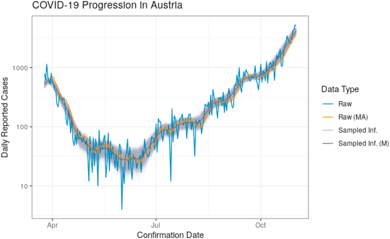
Data on the progression of COVID-19 in Austria is shown in Fig. 1. This graph includes curves for the raw infection data as reported by the European Center for Disease Prevention and Control (Raw), the 7-day moving average of Raw (Raw (MA)), each sampled infection history (Sampled Inf.), and the daily median of the sampled infection histories (Sampled Inf. (M)). Observe that the boundary of the “band” created by the sampled infection histories is not smooth, as it is created from 1000 distinct faded lines. Note that using sampled infection histories effectively shifts the time series backward in time. In order for the infection histories to approximately match the reported case numbers, we have aligned them in time.

Fig. 1.

Summary of new cases of COVID-19 in Austria: raw infection data (Raw), the 7-day moving average of Raw (Raw (MA)), each sampled infection history (Sampled Inf.), and the daily median of the sampled infection histories (Sampled Inf. (M)).

As mentioned in Section 2.1, we sample one million total samples of R and the momentum vector $\vec{\theta }$. To forecast future cases, we use an individual sample of parameters and run the momentum model for a specified period of time. Our graphs show results for the average number of new cases over the following week. As such, they are on the scale of daily reported cases. There is no additional smoothing of the raw data or predictions. As our input is the 7-day moving average, our prediction is the 7-day-ahead forecast of this moving average.

In all of the following graphs, we plot predictions and intervals from three models: the momentum model with k = 0.072, the generation model of Section 2.2 with k = 0.072, and the EpiEstim model of Cori et al. (Cori et al., 2013). As mentioned previously and visible in Appendix D, treating k as random within a relevant region does not alter our results. We label the EpiEstim model “Epi∗”, as the estimates are produced directly via equation (3.1) below instead of using the EpiEstim R package. As in Cori et al. (Cori et al., 2013), we fix a generation interval, as opposed to taking samples of a generation interval estimated from a separate data source as in Thompson et al. (Thompson et al., 2019). As a result, we are not comparing to the best in class model within the EpiEstim/EpiNow framework, but with a model of corresponding complexity to the momentum model. Other improvements to the modeling framework could then be built on top of the momentum model as they have been for the model of Cori et al. (Cori et al., 2013).

To estimate the model of Cori et al. (Cori et al., 2013), we estimate the parameters of the Cori et al. (Cori et al., 2013) posterior distribution directly from the infection data:

$$p\left(R_t|I_{\left[t\right]}\right)=\text{Gamma}\left(a+\sum _{s=t-\tau +1}^t{I}_s,\text{rate}=b+\sum _{s=t-\tau +1}^t\sum _{m=1}^{\nu }{w}_m{I}_{s-m}\right)$$ (3.1)

where a and b are the shape and rate parameter of the gamma prior distribution on R. We estimate this posterior distribution, draw one million samples for R, and run the corresponding data generating process (1.2) for the required number of days.

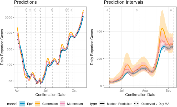
Fig. 2 shows the difference between models with and without superspreading on Austrian data. In order to show a long time period, the data must be plotted on a logarithmic scale such that the low cases in the summer months are visible. As this distorts the plotting of prediction intervals in the same graph, the comparison of prediction intervals is given separately by focusing attention on the summer months between the effective end of COVID restrictions and the start of the school year.

Fig. 2.

Predictions between April 1 and October 31, 2020, and 90% prediction intervals between two significant dates: June 15 and September 7, 2020. Predictions and intervals are for the 7-day average of new cases in the following week in Austria. Relevant event dates are given as vertical, dashed lines and are described in Table 1. The Epi∗ predictions consistently lag behind the observed values, whereas the other methods overshoot in the peaks due to momentum. Models with superspreading produce predictions intervals 2–3 times as wide as those without and achieve better coverage.

For reference, we marked the dates of important changes in COVID-19 restrictions in Austria as vertical, dashed lines. A complete list is available at https://regiowiki.at (in German). The events are described in Table 1. When comparing the events to both reported cases and the estimated reproduction number in Fig. 3, it is necessary to keep the delay distribution in mind; i.e., the effect of an intervention will not be visible in confirmed cases and thereby the estimated reproduction number for roughly two weeks (Abbott et al., 2020). Prior to the removal of any lockdown restrictions, reported case numbers were decaying exponentially. This is visible as a linear decrease given the logarithmic scaling of the y-axis. The slope of this line changed substantially around the time that Austria began to reopen in May and June. From approximately July through the end of October, case numbers fluctuate between growing exponentially and brief periods of relative stability. These fluctuations are not modeled and reflect both noise as well as features which we do not include in our analysis, e.g., common holiday periods, changes in testing, etc. Throughout this period, some restrictions are brought back into effect without apparent substantial impact. Lockdown measures were reinstated at the end of the plotted window of time.

Table 1.

Dates of important events related to COVID-19 in Austria. Changes which occur in large parts of the country but not uniformly are listed as occurring in “some regions”.

Label	Date	Event
NA	2020-03-16	Start of general lock down
1	2020-05-01	Begin relaxation of movement restrictions
2	2020-05-15	Bars and restaurants can open
3	2020-05-29	Hotels and cultural sites can open
4	2020-06-15	Near complete removal of COVID restrictions
5	2020-07-24	Face masks mandatory in essential businesses
6	2020-09-07	Start of school year in some regions
7	2020-09-14	Face masks mandatory
8	2020-09-25	Bars and restaurants close early in some regions
NA	2020-11-03	Start of general soft lock down

Fig. 3.

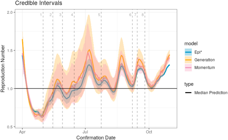
Credible intervals for R in Austria. The momentum and generation model predictions are consistently slightly higher than those of Epi∗. They also produce credible intervals that are 2–3 times as wide. Relevant event dates are given as vertical, dashed lines and are described in Table 1. Observe that R becomes indistinguishable from 1 using our models around the time when lockdown restrictions begin to be removed.

While all of the prediction curves track the observed cases, there are subtle but significant differences in behavior. If one looks closely, one can see that the Epi∗ model predictions lag behind the observed 7-day moving average: it fails to accurately estimate the rapid changes in case numbers. On the other hand, the momentum and generation model predictions “overshoot” the peaks in the time series. As the name suggests, there appears to be excess “momentum” in the process around these change points, and the model anticipates cases to continue rising as in the previous days.

The various models produce prediction intervals with drastically different widths. Most notably, the intervals for the momentum model with k = 0.072 are much wider than those of Epi∗. The generation variant of this model produces intervals which are wider still. The momentum intervals are, on average, approximately three times as wide as those of Epi∗. While the generation model provides a computationally cheap and fast estimate, it is clear that it suffers relative to the momentum model in terms of interval length. The ratio between the prediction interval lengths visible during the summer months is approximately the same throughout the entire prediction period.

To assess the validity of the prediction intervals, Table 2 shows, for each method, the proportion of true weekly new cases that fall within the prediction intervals over the prediction period. Coverage is shown for the 50% and 90% prediction intervals for the raw infection data. When cases are steadily increasing (or decreasing) prediction intervals become narrower, and when the behavior changes they become considerably wider. The prediction intervals of the momentum model cover the true values during periods of growth, while those of Epi∗ often fail to do so over the entire growth period. Clearly coverage is still not exact, and all models perform worse on the Czech data (see Appendix D). It is still notable that the momentum models provide approximate coverage in these cases even with the inherent messiness of the COVID-19 case data. For example, Czechia had a much higher test positivity rate than Austria and Croatia during the majority of the prediction period, which is ignored in our model.

Table 2.

Coverage of the 50% and 90% prediction intervals (PI) for 7-day-ahead predictions of the 7-day moving average. Models with superspreading improve coverage significantly over that of Epi∗.

Country	Model	Coverage, 50% PI	Coverage, 90% PI
Austria	Momentum, k = 0.072	0.46	0.79
	Generation, k = 0.072	0.47	0.73
	Epi∗, k → ∞	0.16	0.38
Croatia	Momentum, k = 0.072	0.48	0.85
	Generation, k = 0.072	0.49	0.77
	Epi∗, k → ∞	0.18	0.47
Czechia	Momentum, k = 0.072	0.40	0.69
	Generation, k = 0.072	0.39	0.66
	Epi∗, k → ∞	0.12	0.32

As the reproduction number is unobserved, we are unable to compare our predictions within a supervised setting as we compared our model forecasts. Given the previous discussion though, we see that the additional variability provided by the momentum model is needed to provide prediction intervals with approximate coverage. Fig. 3 shows the median predictions and 90% credible intervals for R given by the momentum, generation, and Epi∗ models. Intervals are, in general, asymmetric, and skewed toward higher values. The figure clearly demonstrates that the intervals for R are drastically different: with superspreading, intervals for R are roughly 2–3 times as wide as those without. This could have potentially large implications for policy making as we know that relatively small changes in the size of R can lead to large differences in the number of new cases if the disease is allowed to progress unchecked.

Near the beginning of our estimation period and around the time when restrictions were being relaxed in Austria, it quickly becomes infeasible to claim that the reproduction number is below 1; i.e., the credible intervals estimated during May and June include the value 1. Beginning in July and August, however, we observe long periods with reproduction numbers significantly greater than 1, even with our comparatively wide credible intervals. As before, there is a delay of approximately two weeks between when these interventions occur and any change in reproduction number could be observed. Hence any discussion of dates should be interpreted loosely.

As we see a clear improvement in coverage for switching to a model with superspreading, it is useful to have a clearer understanding of the degree of heterogeneity implied by our models. To do so, we consider the posterior samples of R from October 31, 2020. According to equation (1.4), each individual has a separate reproduction number, r_x, given the population reproduction number R. For each posterior sample of R, we therefore draw an individual r_x and secondary infections I_x. The Epi∗ models of Cori et al. (Cori et al., 2013) set r_x = R for all individuals. Hence, it is possible to compare the degree of heterogeneity by considering a Lorenz curve of the population of values of r_x or I_x (Lorenz, 1905).

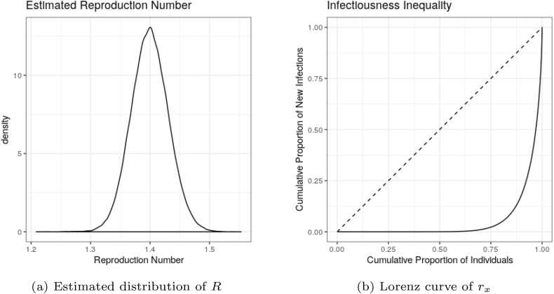
The Lorenz curve is typically used to demonstrate income inequality by showing the proportion of overall income or wealth held by the bottom x% of the people. Here we consider this to be “infectiousness inequality”. The distribution of R estimated for October 31, 2020 as well as the implied Lorenz curve are shown in Fig. 4. The Lorenz curve is a representation of the cumulative distribution function of the number of new expected infections. It allows us to visualize the degree of heterogeneity by seeing which proportion of individuals contribute to new infections. One can draw the Lorenz curve with I_x instead of r_x, which only results in a slightly rougher image with no qualitative differences.

Fig. 4.

Momentum model estimates of R and individual heterogeneity for October 31, 2020. 10% of individuals are expected to contribute approximately 84.6% of new infections. The dashed curve in (b) corresponds to a model without superspreading (Epi∗).

While the population reproduction number is moderately high, this is largely driven by superspreading. The momentum model implies that the top 10% of individuals contribute 84.6% of new infections, while the top 20% contribute 98%. The usefulness of Fig. 4b is that is shows this entire distribution instead of these two common quantiles. We can clearly see that essentially no new cases are produced by nearly 75% of infected individuals. These statistics match quite closely the observed values reported in Arinaminpathy et al. (Arinaminpathy et al., 2020). The figures can also be drawn for the estimation setting in which k is assumed to be randomly drawn from an appropriate gamma distribution. The resulting graphs look essentially identical. As such, treating k as fixed at 0.072 or fluctuating in the approximate range [0.04, 0.2] makes little difference in the infectiousness inequality implied by the momentum model.

4. Conclusion

In this paper, we provide a simple extension of the Cori et al. (Cori et al., 2013) model to account for superspreading. While we explicitly use this to model the COVID-19 pandemic, the methods are easily adaptable to other diseases where superspreading is present. This “momentum” model incorporates unobserved random variables which drive the process of new infections. Even if case numbers and R are relatively small, the presence of superspreaders can increase the momentum of the disease beyond what would be expected if all individuals have the same infectiousness. We observe that this appears necessary to properly track the steep increases or decreases in reported COVID-19 cases. The momentum model produces credible intervals and posterior predictive intervals that are approximately 2–3 times as wide as those that neglect superspreading. We find that these wider intervals significantly improve the coverage of the prediction intervals. The heterogeneity in infectiousness implied by the momentum model is extremely high: 10% of individuals contribute approximately 84.6% of new infections.

As Bayesian models are time and resource intensive to estimate, we also derive a simplified model in which infected individuals are only infectious for a single day. In order to improve the fit to real data, we partition disease incidence into generations, each of which spans multiple days. The length of each generation corresponds to the generation time of the disease, and within this period an infected person is assumed to be equally infectious. This yields two main benefits. First, estimation of R and predictions of new cases are immediately available through an explicit approximation of the posterior distribution of R. Second, this model allows us to derive a simple equation to relate the width of credible intervals to the degree of superspreading. Hence, we have rigorous analysis which supports the heuristic that the approximate length of a credible interval for R behaves like

$$\frac{2z_{1-\alpha /2}}{\sqrt{k{\sum }_{s=t-\tau +1}^t{I}_s}},$$

where z_1−α/2 is the (1 − α/2) quantile of the standard normal distribution and for values of dispersion parameter k much smaller than 1, which corresponds to scenarios with high superspreading. The model assumes that R has been constant for the preceding τ days.

Declaration of competing interest

The authors declare that they have no known competing financial interests or personal relationships that could have appeared to influence the work reported in this paper.

Handling editor: Dr HE DAIHAI HE

Appendix A. Likelihood derivation

This appendix derives the posterior distribution of R and ${\vec{\theta }}_{\left[t-\tau -\nu +1,t-1\right]}$ given the relevant observable past, i.e., ${\vec{I}}_{\left[t-\tau -\nu +1,t\right]}$. We briefly restate some basic properties and definitions of our model.

Let w_i denote the expected proportion of future infections caused by an infected person which occur on day i after infection. Let ν denote the length of infectiousness, i.e., w_ν+k = 0 for all k > 0. Lastly, τ denotes the number of days over which we assume R is constant.

Our distributional assumptions are as follows:

$$\begin{array}{cc}{I}_t|{\vec{\theta }}_{\left[0,t-1\right]},{\vec{I}}_{\left[0,t\right]},R& ~\text{Poisson}\left(\sum _{s=1}^{\nu }{\omega }_s{\theta }_{t-s}\right),\text{ i.e., }\\ p\left(I_t|{\vec{\theta }}_{\left[0,t-1\right]},{\vec{I}}_{\left[0,t\right]},R\right)& =\frac{1}{I_t!}{\left(\sum _{s=1}^{\nu }{\omega }_s{\theta }_{t-s}\right)}^{I_t}{e}^{-\sum _{s=1}^{\nu }{\omega }_s{\theta }_{t-s}};\text{ and}\\ {\theta }_s|R,{\vec{I}}_{\left[0,s\right]},{\vec{\theta }}_{\left[0,s-1\right]}& ~\text{Gamma}\left(I_{s}k,\text{rate}=\frac{k}{R}\right),\text{ i.e., }\\ p\left({\theta }_s|R,{\vec{I}}_{\left[0,s\right]},{\vec{\theta }}_{\left[0,s-1\right]}\right)& =\frac{{\left(\frac{k}{R}\right)}^{I_{s}k}}{\mathrm{\Gamma }\left(I_{s}k\right)}{\theta }_s^{I_{s}k-1}{e}^{-\frac{{\theta }_{s}k}{R}}.\end{array}$$

We want to calculate the joint distribution:

$$\begin{array}{ccc}& p& \left({\vec{\theta }}_{\left[t-\tau -\nu +1,t-1\right]},R|{\vec{I}}_{\left[t-\tau -\nu +1,t\right]}\right)\\ & =& p\left({\vec{\theta }}_{\left[t-\tau -\nu +1,t-1\right]},R|{\vec{I}}_{\left[t-\tau -\nu +1,t-\tau \right]},{\vec{I}}_{\left[t-\tau +1,t\right]}\right)\\ & \propto & p\left({\vec{I}}_{\left[t-\tau +1,t\right]}|{\vec{I}}_{\left[t-\tau -\nu +1,t-\tau \right]},{\vec{\theta }}_{\left[t-\tau -\nu +1,t-1\right]},R)p({\vec{\theta }}_{\left[t-\tau -\nu +1,t-1\right]},R|{\vec{I}}_{\left[t-\tau -\nu +1,t-\tau \right]}\right)\\ & =& p\left({\vec{I}}_{\left[t-\tau +1,t\right]},{\vec{\theta }}_{\left[t-\tau -\nu +1,t-1\right]},R|{\vec{I}}_{\left[t-\tau -\nu +1,t-\tau \right]}\right)\\ & =& p\left(I_t,{\theta }_{t-1}|{\vec{I}}_{\left[t-\tau -\nu +1,t-1\right]},{\vec{\theta }}_{\left[t-\tau -\nu +1,t-2\right]},R\right)\\ & & \cdot p\left({\vec{I}}_{\left[t-\tau +1,t-1\right]},{\vec{\theta }}_{\left[t-\tau -\nu +1,t-2\right]},R|{\vec{I}}_{\left[t-\tau -\nu +1,t-\tau \right]}\right)\\ & =& p\left(I_t|{\vec{\theta }}_{\left[t-\nu ,t-1\right]}\right)p\left({\theta }_{t-1}|I_{t-1},R\right)p\left({\vec{I}}_{\left[t-\tau +1,t-1\right]},{\vec{\theta }}_{\left[t-\tau -\nu +1,t-2\right]},R|{\vec{I}}_{\left[t-\tau -\nu +1,t-\tau \right]}\right).\end{array}$$

In the last step we used the conditional independence properties for I_t and θ_t−1, respectively. Repeating this process to separate I_[t−τ+2,t] and θ_{[t−τ+1,t−1]} from the rest yields:

$$\begin{array}{ccc}& p& \left({\vec{\theta }}_{\left[t-\tau -\nu +1,t-1\right]},R|{\vec{I}}_{\left[t-\tau -\nu +1,t\right]}\right)\\ & \propto & \prod _{s=t-\tau +2}^{t}p\left(I_s|{\vec{\theta }}_{\left[s-\nu ,s-1\right]}\right)\\ & & \cdot \prod _{s=t-\tau +1}^{t-1}p\left({\theta }_s|I_s,R)p(I_{t-\tau +1},{\vec{\theta }}_{\left[t-\tau -\nu +1,t-\tau \right]},R|{\vec{I}}_{\left[t-\tau -\nu +1,t-\tau \right]}\right)\end{array}$$

Now, focusing on the last term, we have

$$\begin{array}{ccc}& p& \left(I_{t-\tau +1},{\vec{\theta }}_{\left[t-\tau -\nu +1,t-\tau \right],R|{\vec{I}}_{\left[t-\tau -\nu +1,t-\tau \right]}}\right)\\ & =& p\left(I_{t-\tau +1},{\vec{\theta }}_{\left[t-\tau -\nu +1,t-\tau \right]}|{\vec{I}}_{\left[t-\tau -\nu +1,t-\tau \right]},R)p(R|{\vec{I}}_{\left[t-\tau -\nu +1,t-\tau \right]}\right)\\ & =& p\left(I_{t-\tau +1}|{\vec{I}}_{\left[t-\tau -\nu +1,t-\tau \right]},{\vec{\theta }}_{\left[t-\tau -\nu +1,t-\tau \right]},R)p({\vec{\theta }}_{\left[t-\tau -\nu +1,t-\tau \right]}|{\vec{I}}_{\left[t-\tau -\nu +1,t-\tau \right]},R\right)\\ & & \cdot p\left(R|{\vec{I}}_{\left[t-\tau -\nu +1,t-\tau \right]}\right)\\ & =& p\left(I_{t-\tau +1}|{\vec{\theta }}_{\left[t-\tau -\nu +1,t-\tau \right]}\right)\prod _{s=t-\tau -\nu +1}^{t-\tau }p\left({\theta }_s|{\vec{I}}_{\left[t-\tau -\nu +1,t-\tau \right]},R\right)p\left(R|{\vec{I}}_{\left[t-\tau -\nu +1,t-\tau \right]}\right).\end{array}$$

In the last equation, we used the fact that the individual θ_s are conditionally independent given the vector $\vec{I}$. At this point, the terms $p\left({\theta }_s|{\vec{I}}_{\left[t-\tau -\nu +1,t-\tau \right]},R\right)$ become problematic. Knowledge of the terms I_m for m > s certainly should shed some insight on the value of θ_s; however, it is not clear how this can be feasibly handled. It is not possible to prevent the occurrence of such terms due to the hierarchical nature of this model: the distribution of I_s requires previous θ values, which in return demand the inclusion of previous I values ad infinitum. This problem could be avoided by modeling all data from the start of the epidemic, at which point we could confidently set all values of I and θ corresponding to times prior to the onset of the epidemic to 0. This, however, would require treating the value of R as fixed for the entire epidemic, rendering our approach irrelevant as this assumption is clearly false.

As a solution, we propose putting a prior distribution on these problematic θ_s such that $p\left({\theta }_s|{\vec{I}}_{\left[t-\tau -\nu +1,t-\tau \right]},R\right)~\mathrm{\Gamma }\left(I_{s}k,k/R\right)$, essentially disregarding the additional information provided by future observations. Using a different prior, such as setting $p\left({\theta }_s|{\vec{I}}_{\left[t-\tau -\nu +1,t-\tau \right]},R\right)={\delta }_{R{I}_s}$—which has the appeal of creating terms such as those in Cori et al. (2013)—is statistically unsound, as we would draw different θ_s from different types of distributions.

All this taken together yields:

$$\begin{array}{ccc}& p& \left({\vec{\theta }}_{\left[t-\tau -\nu +1,t-1\right]},R|{\vec{I}}_{\left[t-\tau -\nu +1,t\right]}\right)\\ & \propto & \prod _{s=t-\tau +1}^{t}p\left(I_s|{\vec{\theta }}_{\left[s-\nu ,s-1\right]}\right)\prod _{s=t-\tau +1}^{t-1}p\left({\theta }_s|I_s,R\right)\prod _{s=t-\tau -\nu +1}^{t-\tau }p\left({\theta }_s|I_s,R\right)\\ & & \cdot p\left(R|{\vec{I}}_{\left[t-\tau -\nu +1,t-\tau \right]}\right)\end{array}$$

Using an inverse-gamma prior on R and using the densities of the other terms as discussed before evaluates to the same likelihood as in the main text.

Appendix B. Model validation

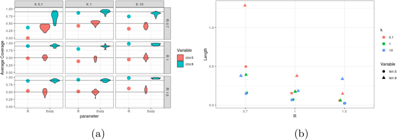
Here we summarize estimation results for simulated data in order to more precisely show the effect of superspreading in a setting in which true parameters are known. The coverage and length of intervals are shown in Fig. B5. All simulations use an initial sequence of τ observations that have constant value 50. The momentum model is simulated for a further 3τ days. This complete series is then used to estimate R and $\vec{\theta }$. Simulations were repeated 50 times in order to asses coverage probabilities.

Of greatest initial import is verifying that the 90% credible intervals for R indeed cover the true value with approximately nominal probability. The case R = 1 is of primary importance, as it represents the bright-line between the epidemic growing or shrinking. That we have nearly exact coverage in this setting is indication that our credible intervals do not achieve coverage merely by being extremely wide. Furthermore, the intervals for $\vec{\theta }$ also cover the true values with the specified probability when R = 1 or R = 1.5. With our initial sequence of cases and R = 0.7, the epidemic sometimes dies out, which can be missed by the model. As such, coverage somewhat worse in this case.

Fig. B.5.

Illustration of average credible interval coverage (cov.-) and length (len.-) on simulated data. As there is a single R parameter but 25 elements of $\vec{\theta }$, the coverage of the latter are summarized via a violin plot.

After establishing coverage, our motivation for modeling superspreading is verified by looking at the lengths of the credible intervals: for k small, our intervals need to be extremely wide. In fact, the interval for k = 0.1 is approximately 2.5 times longer than the interval for k = 10 for both R = 0.7 and R = 1. For R = 1.5, the estimation problem becomes relatively easy as case numbers grow substantially. This leads to very small credible intervals.

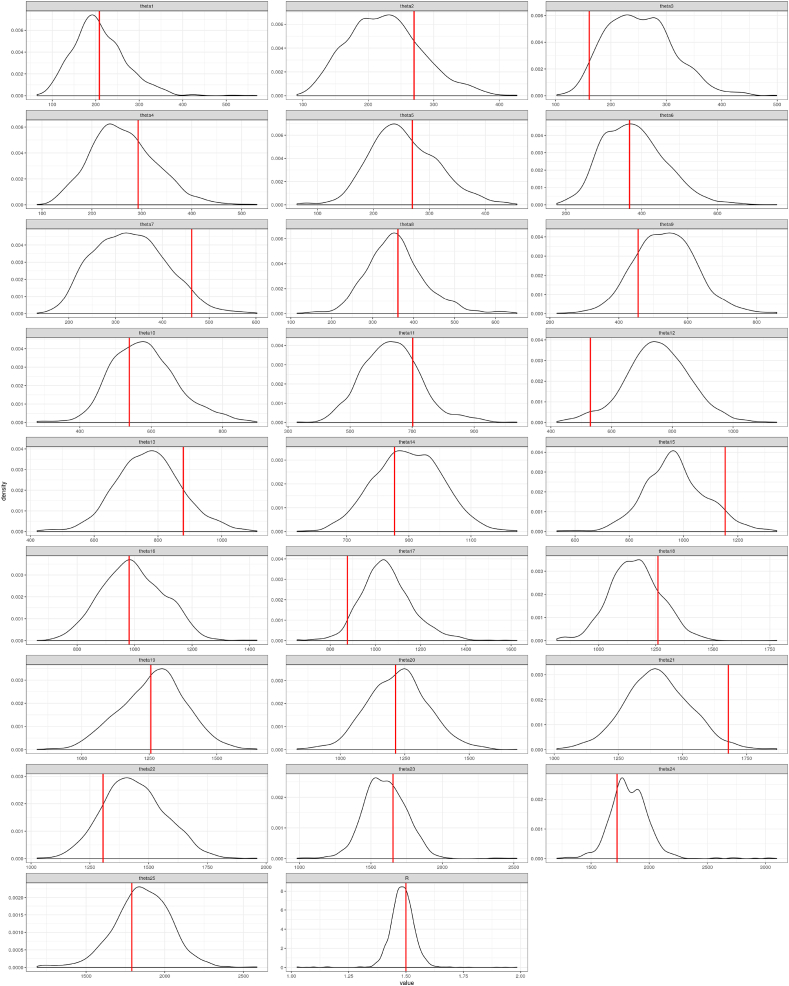
As the explicit conditional distribution of the momentum parameters $\vec{\theta }$ is intractable, we present a summary of the samples observed through the MCMC simulation in Fig. B6. This includes all 25 momentum parameters required when τ = ν = 13 as well as R. As R = 1.5 in this setting, one can observe that the scale increases for θ_s as s increases. It is clear that the parameters vary widely through MCMC estimation, even though the are initialized at the marginal MLE: ${\widehat{\theta }}_s=I_s\widehat{R}$. Multiple chains are run, each with a separate initial value for $\widehat{R}$. When k is small, variability in $\vec{\theta }$ is large, requiring both tuning of the proposal distribution and long chains to be simulated in order to overcome high auto-correlation in the MCMC draws of $\vec{\theta }$.

Fig. B.6.

Samples of MCMC draws of parameters. The vertical, red lines indicate true values.

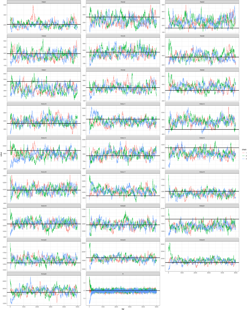
Fig. B7 shows how the individuals MCMC chains behave for each of the 25 momentum parameters in $\vec{\theta }$. Graphs for all parameters are shown in order to demonstrate that there is insufficient information to estimate the full set of parameters. One can also see how quickly the parameter estimates from different chains converge even when started a significantly different—and in some cases completely incorrect—starting values. Depending on the value of k, the variance of the proposal distribution for $\vec{\theta }$ must be set in order to allow θ to move slowly. If the variance is too high, then the acceptance proportion of proposed parameters is extremely low. This is due to the vector jumping to a nonsensical configuration, even if each individual θ_i is plausible in isolation.

Fig. B.7.

Each posterior distribution is composed of samples from several chains. As seen above, the chains converge quickly.

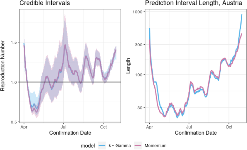
As a final model validation, we consider k being drawn from a suitable distribution instead of being fixed. By using k ~ Gamma(6, rate = 55) we achieve approximately the same 2.5%, 50%, and 97.5% quantiles of the distribution of k given in Endo et al. (2020). For reference, these are 0.04, 0.1, and 0.2, respectively. Fig. B8 shows credible intervals for R and prediction interval lengths for the momentum model with k = 0.072 and k random as above. Only these summary graphs are shown because no differences are visible in the missing figures. The only notable difference in the estimation of the reproduction number occurs when observed cases are very low. In this region, treating k as random yields slightly larger estimates for R as well as wider confidence intervals. Lastly, we note that the intervals for R are not as symmetric as for the k-fixed case as they are skewed slightly left. Furthermore, there is less heterogeneity in infectiousness. Our models estimate that 10% of infected individuals contribute 81% of new infections while 20% contribute 95% of new infections.

Fig. B.8.

Comparison of selected graphs for k fixed and k ~ Gamma().

Appendix C. Generation model derivations

Appendix C.1. Normal approximation

This appendix derives the normal approximation to the posterior distribution $p\left(R|{\vec{I}}_{\left[t\right]},k\right)$ used in Section 2.2. As we can iteratively condition on previous values, the joint distribution of ${\vec{I}}_{\left[t-\tau +1,t\right]}|{\vec{I}}_{t-\tau },R,k$ decomposes into a product of factors of the form (2.7). We have

$$\begin{array}{ccc}p\left({\vec{I}}_{\left[t-\tau +1,t\right]}|{\vec{I}}_{\left[t-\tau \right]},R,k\right)& =& \prod _{s=t-\tau +1}^{t}p\left(I_s|{\vec{I}}_{\left[s-1\right]},R,k\right)\\ & =& \prod _{s=t-\tau +1}^t\frac{\mathrm{\Gamma }\left(I_s+k{I}_{s-1}\right)}{I_s!\mathrm{\Gamma }\left(k{I}_{s-1}\right)}{\left(\frac{k}{R+k}\right)}^{k{I}_{s-1}}{\left(\frac{R}{R+k}\right)}^{I_s}.\end{array}$$

The structure of this likelihood suggests estimating R/(R + k) instead of R. When treating ${\vec{I}}_{\left[t-\tau \right]}$ and k as fixed, Bayes’ theorem yields the posterior distribution of R/(R + k):

$$\begin{array}{ccc}& p& \left(\frac{R}{R+k}|{\vec{I}}_{\left[t\right]},k\right)\\ & \propto & {\left(\frac{k}{R+k}\right)}^{k\sum _{s=t-\tau }^{t-1}{I}_s}{\left(\frac{R}{R+k}\right)}^{\sum _{s=t-\tau +1}^t{I}_s}p\left(\frac{R}{R+k}|I_{\left[t-\tau \right]},k\right).\end{array}$$ (C.1)

Fig. C.9.

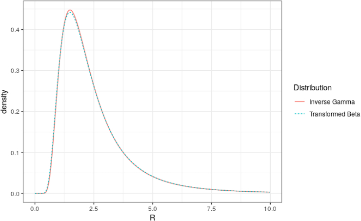
Comparison of priors on R and R/(R + k).

Given this functional form, it is natural to put a beta prior on R/(R + k) to maintain conjugacy. For small k, as shown in Fig. C9, this corresponds to putting an appropriate inverse-gamma prior on R, while for larger k this would correspond to a gamma prior. Therefore, to mimic the R ~Inv-Gamma(3.69, rate = 6.994) prior distribution used in Section 2.1, we can use a Beta $\left(\tilde{\alpha }=98.82,\tilde{\beta }=3.74\right)$ prior on R/(R + k). The posterior distribution of R/(R + k) then has a Beta distribution with parameters

$$\alpha =\tilde{\alpha }+\sum _{s=t-\tau +1}^t{I}_s,\beta =\tilde{\beta }+k\sum _{s=t-\tau }^{t-1}{I}_s.$$

While the hyperparameter values are not so small as to be uninformative, they are easily outweighed by the data in most settings. By a change of variables from R/(R + k) back to R, we derive the posterior distribution of R to be

$$p\left(R|{\vec{I}}_{\left[t\right]},k\right)\propto \frac{k}{{\left(R+k\right)}^2}{\left(\frac{R}{R+k}\right)}^{\alpha -1}{\left(\frac{k}{R+k}\right)}^{\beta -1}.$$ (C.2)

As a final simplifying step, we compute the normal approximation of this posterior [8, Section 4.1]. To this end, the first and second derivatives of the log-posterior density are

$$\begin{array}{ccc}\frac{d}{dR}\log p\left(R|{\vec{I}}_{\left[t\right],k}\right)& =& \frac{\alpha -1}{R}-\frac{\alpha +\beta }{R+k},\\ \frac{d^2}{d{R}^2}\log p\left(R|{\vec{I}}_{\left[t\right]},k\right)& =& -\frac{\alpha -1}{R^2}+\frac{\alpha +\beta }{{\left(k+R\right)}^2}.\end{array}$$

Thus, the mode of the posterior is

$$\begin{array}{ccc}\widehat{R}=\frac{k\left(\alpha -1\right)}{\beta +1},& & \end{array}$$

and the variance estimate is

$$\begin{array}{ccc}{\left(-\frac{d^2}{d{R}^2}p\left(R|{\vec{I}}_{\left[t\right]},k\right)\left(\widehat{R}\right)\right)}^{-1}=\frac{k^2\left(\alpha +\beta \right)\left(\alpha -1\right)}{{\left(\beta +1\right)}^3}.& & \end{array}$$

This yields a normal approximation of the posterior of

$$\begin{array}{ccc}p\left(R|{\vec{I}}_{\left[t\right]},k\right)& \approx & N\left(\frac{k\left(\alpha -1\right)}{\beta +1},\frac{k^2\left(\alpha +\beta \right)\left(\alpha -1\right)}{{\left(\beta +1\right)}^3}\right).\end{array}$$

Appendix C.2. Generation model

It is easiest to represent the process of infections per generation if we allow the indices of the summation notation to be real numbers (hence treating the summation as integration) via

$$\begin{array}{ccc}\sum _{s=c_1}^{c_2}{I}_{t-s}& =& \left(\lceil c_1\rceil -c_1\right)I_{t-\lceil c_1\rceil +1}+\sum _{s=\lceil c_1\rceil }^{\lfloor c_2\rfloor -1}{I}_{t-s}+\left(c_2-\lfloor c_2\rfloor \right)I_{t-\lfloor c_2\rfloor }\end{array}$$

for $c_1,c_2\in \mathbb{R}$ where c₁ < c₂. When D_g is the length of a generation, the number of infections per generation is then given simply by

$$\begin{array}{ccc}{\tilde{I}}_{\tilde{t}-i}& =& \sum _{s=i\cdot D_g}^{\left(i+1\right)\cdot D_g}{I}_{t-s},\end{array}$$

for $i\in {\mathbb{N}}_0$.

We assume R is constant for τ days in the generation model as in the momentum model. The corresponding parameter in the generation model is τ_g≔τ/D_g, where we account for non-integer values as before by summing fractional daily infections. Estimating parameters and producing forecasts requires similar modifications for non-integer values. Conceptually, however, these correspond to the same sums as before, just over generations instead of conventional days. This can be represented concisely in the notation for real-valued summation as

$$\begin{array}{ccc}\alpha & =& \tilde{\alpha }+\sum _{s=0}^{{\tau }_{meta}}{\tilde{I}}_{\tilde{t}-s},\text{and}\end{array}$$ (C.3)

$$\begin{array}{ccc}\beta & =& \tilde{\beta }+k\sum _{s=1}^{{\tau }_{meta}+1}{\tilde{I}}_{\tilde{t}-s}.\end{array}$$ (C.4)

This yields a negative binomial observation model as before:

$${\tilde{I}}_{\tilde{t}}|R,{\tilde{I}}_{\tilde{t}-1}~NB\left({\tilde{I}}_{\tilde{t}-1}k,\frac{R}{k+R}\right).$$

For prediction and comparisons used in Section 3, it is more sensible to compare the cumulative incidence of several, say T, days. We forecast $\lceil \frac{\mathbf{T}}{D_g}\rceil$ generations ${\tilde{I}}_{\tilde{t}}$, and our forecast for T days is then

$$X_{\mathbf{T}}=\sum _{s=1}^{\lfloor \frac{\mathbf{T}}{D_g}\rfloor }{\tilde{I}}_{\tilde{t}+s}+\left(\frac{\mathbf{T}}{D_g}-\frac{\mathbf{T}}{D_g}\right){\tilde{I}}_{\tilde{t}+\lceil \frac{\mathbf{T}}{D_g}\rceil }.$$

In the case study of Section 3, we forecast the total weekly cases, i.e., T = 7. Observe that this equates to merely forecasting sufficient generations to cover the desired time period, then taking the appropriate proportion of the final forecasted generation to match the desired time window T.

Appendix D. Results for Croatia and Czechia

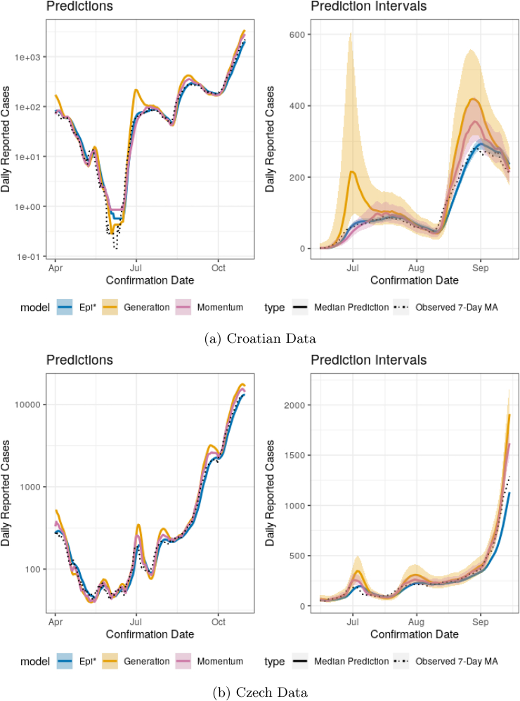
As further demonstration of the momentum model, Figs. D10 and D11 show the same prediction and estimation results as seen in Section 3 but for Croatia and Czechia. The disease progression in Czechia is similar to that of Austria over the shown period. Croatia is a common Austrian and Czech tourist destination and the disease progression is markedly different there than in Austria. The estimated coverage probabilities of the prediction intervals are also shown in Table 2. The story remains the same as before: coverage is far better for the momentum model with superpreading than without (Epi∗). Similarly, Epi∗ appears shifted relative to the observed cases, particularly for the Czech data. Here we see that the momentum model performs better than the generation model, particularly around peaks in the time series.

Fig. D.10.

Predictions between April 1 and October 31, 2020, and 90% prediction intervals between June 15 and September 7, 2020. Predictions and intervals are for the 7-day average of new cases in the following week in Croatia and Czechia.

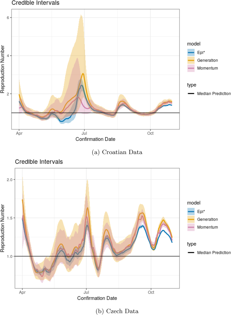
Fig. D11 contains results on the estimation of R for Croatia and Czechia. The results are qualitatively the same, in that the momentum model with superspreading produces much wider credible intervals. One obvious feature of the Croatian data, however, is a steep decline and subsequent steep increase in June. This corresponds to a large increase and plateau in cases as seen in Fig. D10. The Epi∗ model estimates that R increases to well over 2 within a short period of time before decreasing again to previous levels. Alternatively, in the same period, the momentum model provides a noticeably lower median estimate but with an incredibly wide interval. Further exploration of the feature is warranted, though it is reasonable that such a large deviation over a small window of time should produce significantly more uncertainty in the value of the underlying parameter, particularly when the model is estimated under the assumption that R is constant over τ = 13 days. Within the momentum model, such short-term deviations can be captured by an increase or decrease in disease momentum instead of just an increase in R. On the other hand, this feature appears to show a flaw within the generation model, as both the estimated R and interval estimate have extreme spikes. This is likely due to the short-term nature of the case increase and the generation model only using roughly three generations for estimation.

Fig. D.11.

Credible intervals and for R in Croatia and Czechia between April 1 and October 31, 2020.

References

- Abbott S., Hellewell J., Thompson R.N., Sherratt K., Gibbs H.P., Bosse N.I., Funk S., CMMID COVID modelling group Estimating the time-varying reproduction number of sars-cov-2 using national and subnational case counts. Wellcome Open Res. 2020;5(112):112. [Google Scholar]
- Adam D.C., Wu P., Wong J.Y., Lau E.H., Tsang T.K., Cauchemez S., Leung G.M., Cowling B.J. Clustering and superspreading potential of sars-cov-2 infections in Hong Kong. Nat. Med. 2020;26(11):1714–1719. doi: 10.1038/s41591-020-1092-0. [DOI] [PubMed] [Google Scholar]
- Arinaminpathy N., Das J., McCormick T., Mukhopadhyay P., Sircar N. 2020. Quantifying heterogeneity in sars-cov-2 transmission during the lockdown in India. medRxiv. [DOI] [PMC free article] [PubMed] [Google Scholar]
- Cori A., Ferguson N.M., Fraser C., Cauchemez S. A new framework and software to estimate time-varying reproduction numbers during epidemics. Am. J. Epidemiol. 2013;178(9):1505–1512. doi: 10.1093/aje/kwt133. [DOI] [PMC free article] [PubMed] [Google Scholar]
- Donnat C., Holmes S. 2020. Modeling the heterogeneity in covid-19’s reproductive number and its impact on predictive scenarios. arXiv preprint arXiv:2004.05272. [DOI] [PMC free article] [PubMed] [Google Scholar]
- Endo A., Abbott S., Kucharski A., Funk S. Estimating the overdispersion in covid-19 transmission using outbreak sizes outside China. Wellcome Open Res. 2020;5:67. doi: 10.12688/wellcomeopenres.15842.1. [DOI] [PMC free article] [PubMed] [Google Scholar]
- Ganyani T., Kremer C., Chen D., Torneri A., Faes C., Wallinga J., Hens N. Estimating the generation interval for coronavirus disease (covid-19) based on symptom onset data, march 2020. Euro Surveillance. 2020;25(17):2000257. doi: 10.2807/1560-7917.ES.2020.25.17.2000257. [DOI] [PMC free article] [PubMed] [Google Scholar]
- Gelman A., Carlin J.B., Stern H.S., Rubin D.B. 2nd ed. edition. Chapman and Hall/CRC; 2004. Bayesian data analysis. [Google Scholar]
- Gostic K.M., McGough L., Baskerville E.B., Abbott S., Joshi K., Tedijanto C., Cobey S. Vol. 16. PLOS Computational Biology; 2020. Practical considerations for measuring the effective reproductive number, Rt; pp. 1–21. [DOI] [PMC free article] [PubMed] [Google Scholar]
- Knight J., Mishra S. Estimating effective reproduction number using generation time versus serial interval, with application to covid-19 in the greater toronto area, Canada. Infect. Dis. Model. 2020;5:889–896. doi: 10.1016/j.idm.2020.10.009. [DOI] [PMC free article] [PubMed] [Google Scholar]
- Laxminarayan R., Wahl B., Dudala S.R., Gopal K., Mohan C., Neelima S., Reddy K.S.J., Radhakrishnan J., Lewnard J. 2020. Epidemiology and transmission dynamics of covid-19 in two indian states. medRxiv. [DOI] [PMC free article] [PubMed] [Google Scholar]
- Liu Y., Eggo R.M., Kucharski A.J. Secondary attack rate and superspreading events for sars-cov-2. The Lancet. 2020;395(10227):e47. doi: 10.1016/S0140-6736(20)30462-1. [DOI] [PMC free article] [PubMed] [Google Scholar]
- Lloyd-Smith J.O., Schreiber S.J., Kopp P.E., Getz W.M. Superspreading and the effect of individual variation on disease emergence. Nature. 2005;438(7066):355–359. doi: 10.1038/nature04153. [DOI] [PMC free article] [PubMed] [Google Scholar]
- Lorenz M.O. Methods of measuring the concentration of wealth. Publ. Am. Stat. Assoc. 1905;9(70):209–219. [Google Scholar]
- Ma J. Estimating epidemic exponential growth rate and basic reproduction number. Infect. Dis. Model. 2020;5:129–141. doi: 10.1016/j.idm.2019.12.009. [DOI] [PMC free article] [PubMed] [Google Scholar]
- O’Driscoll M., Harry C., Donnelly C.A., Cori A., Dorigatti I. 2020. A comparative analysis of statistical methods to estimate the reproduction number in emerging epidemics with implications for the current covid-19 pandemic. medRxiv. [DOI] [PMC free article] [PubMed] [Google Scholar]
- Richter L., Schmid D., Chakeri A., Maritschnik S., Pfeiffer S., Stadlober E. 2020. Schätzung des seriellen intervalles von covid10.https://www.ages.at/en/wissen-aktuell/publikationen/schaetzung-des-seriellen-int ervalles-von-covid19-oesterreich/ Österreich. Technical report. [Google Scholar]
- Thompson R.N., Stockwin J.E., van Gaalen R.D., Polonsky J.A., Kamvar Z.N., Demarsh P.A., Cori A. Improved inference of time-varying reproduction numbers during infectious disease outbreaks. Epidemics. 2019;29:100356. doi: 10.1016/j.epidem.2019.100356. [DOI] [PMC free article] [PubMed] [Google Scholar]
- Wallinga J., Lipsitch M. 2007. How generation intervals shape the relationship between growth rates and reproductive numbers. [DOI] [PMC free article] [PubMed] [Google Scholar]
- Wallinga J., Teunis P. Different epidemic curves for severe acute respiratory syndrome reveal similar impacts of Control measures. American Journal of Epidemiology. 2004;160(6):509–516. doi: 10.1093/aje/kwh255. [DOI] [PMC free article] [PubMed] [Google Scholar]