“Distances, distance distributions, and ensembles of unfolded and intrinsically disordered proteins from single-molecule FRET”

Abstract

Intrinsically disordered proteins (IDPs) sample structurally diverse ensembles. Characterizing the underlying distributions of conformations is a key step towards understanding the structural and functional properties of IDPs. One increasingly popular method for obtaining quantitative information on intramolecular distances and distributions is single-molecule Förster resonance energy transfer (FRET). Here we describe two essential elements of the quantitative analysis of single-molecule FRET data of IDPs: the sample-specific calibration of the single-molecule instrument that is required for determining accurate transfer efficiencies, and the use of state-of-the-art methods for inferring accurate distance distributions from these transfer efficiencies. First, we illustrate how to quantify the correction factors for instrument calibration with alternating donor and acceptor excitation measurements of labeled samples spanning a wide range of transfer efficiencies. Second, we show how to infer distance distributions based on suitably parameterized simple polymer models, and how to obtain ensembles from Bayesian reweighting of molecular simulations or from parameter optimization in simplified coarse-grained models.

Introduction

For more than a century (Fischer, 1902), one of the fundamental concepts of molecular biology, and in particular enzymology, has been that the functions of proteins are closely coupled to their folded, three-dimensional structures. However, it is now clear that proteins can be functional without stable tertiary or even secondary structure (Dyson & Wright, 2005; Forman-Kay & Mittag, 2013; Tompa, 2005). Such intrinsically disordered proteins (IDPs) are involved in many essential biological processes, particularly in higher eukaryotes (Dunker et al., 2001; Oates et al., 2013; van der Lee et al., 2014). Nevertheless, understanding their functional mechanisms requires a rigorous and quantitative analysis of the structurally diverse ensembles they populate.

There are many powerful methods available for characterizing the broad conformational distributions and dynamics of IDPs (Gibbs & Showalter, 2015; Uversky, 2012), such as NMR (Konrat, 2014) and SAXS (Kikhney & Svergun, 2015). NMR provides a wealth of detailed structural information, especially regarding short-range interactions, secondary structure content, and conformational dynamics over a broad range of timescales. SAXS can report on the overall dimensions and shape of a biomolecule. It is becoming increasingly apparent that these methods can be ideally complemented by single-molecule Förster resonance energy transfer (FRET), which has been used successfully as a “spectroscopic ruler” to probe the dimensions and dynamics of IDPs (Ferreon, Moran, Gambin, & Deniz, 2010; Schuler, Soranno, Hofmann, & Nettels, 2016). Key strengths of such single-molecule experiments are the ability to quantify specific long-range intra- and intermolecular distances, to distinguish static and dynamic heterogeneity, to resolve coexisting subpopulations, and to probe conformational dynamics ranging from rapid conformational fluctuations on the nanosecond timescale all the way to the formation of higher-order assemblies on the timescale of days and weeks (Schuler & Hofmann, 2013). Finally, the small volumes and low concentrations used in single-molecule FRET require only minute amounts of sample; provide access to concentrations down to the picomolar range; and can easily be used in a broad spectrum of solutions conditions, even within live cells (König et al., 2015; Sustarsic & Kapanidis, 2015). Together, these advantages have made single-molecule FRET a versatile tool for biophysical studies of conformationally heterogeneous biological molecules like IDPs.

In many applications, qualitative distance information provided by single-molecule FRET is sufficient (e.g. many kinetic analyses), but FRET can also be used to obtain quantitative distance information, not only for structured biomolecules (Hellenkamp, Wortmann, Kandzia, Zacharias, & Hugel, 2017; Kalinin et al., 2012; Muschielok et al., 2008), but also for IDPs (Gomes & Gradinaru, 2017; Schuler et al., 2016), as demonstrated by comparison with other methods (Aznauryan et al., 2016; Borgia et al., 2016; Fuertes et al., 2017). However, this task requires two key steps: First, an accurate transfer efficiency must be obtained from the experimental data acquired on a calibrated instrument. Second, the distance distribution within the IDP must be inferred from this transfer efficiency based on a reasonable model. The first step poses essentially the same challenges for IDPs as for structured biomolecules (Hellenkamp et al., 2018); additionally, a detailed analysis of photon statistics can be used to identify the presence of broad distance distributions (Gopich & Szabo, 2012; Schuler et al., 2016). The second step is even more demanding, since information about a broad distribution of distances must be inferred, corresponding to a highly underdetermined inverse problem. However, advances in the use of analytical polymer models and molecular simulations can now be employed to infer increasingly accurate distance distributions of unfolded and intrinsically disordered proteins from single-molecule FRET experiments, ideally in combination with data from complementary methods (Borgia et al., 2016; Fuertes et al., 2017; Zheng et al., 2018). In this chapter, we outline the steps required for performing accurate transfer efficiency measurements of fluorescently labeled IDPs and for inferring the underlying distance distributions.

FRET

Förster Resonance Energy Transfer (FRET) is a photophysical phenomenon involving the non-radiative dipole-dipole coupling between chromophores (Förster, 1948) that is often exploited to measure distances on biomolecular length scales. An electronically excited donor chromophore (D*) transfers energy to a nearby acceptor chromophore in the ground state (A), resulting in de-excitation of the donor (D) and excitation of the acceptor (A*). The rate coefficient for energy transfer, k_FRET, from D* to A depends on the donor fluorescence lifetime, τ_D, and the sixth power of the Förster radius, R₀, divided by the distance, r, between the two fluorophores:

$$k_{\mathit{\text{FRET}}}=\frac{\text{1}}{{\tau }_{\text{D}}}{\left(\frac{R_{\text{0}}}{r}\right)}^{\text{6}}.$$ (1)

The FRET efficiency, ε, at a given r is the probability that a D*→ D transition will occur via energy transfer (k_FRET) rather than other non-radiative (k_nrad) or radiative (k_rad) decay processes, and thus ε = ½ when r = R₀:

$$\epsilon =\frac{k_{\mathit{\text{FRET}}}}{k_{\mathit{\text{FRET}}}+k_{\mathit{\text{rad}}}+k_{\mathit{\text{nrad}}}}\text{=}\frac{{R_0}^6}{{R_0}^6\text{+}{r}^{\text{6}}}.$$ (2)

The value of R₀ can be calculated from the refractive index of the medium, the donor quantum yield, the relative orientation of the two fluorophores, and the overlap integral of the donor emission and acceptor absorption spectra (Van Der Meer, 1994). If R₀ is known, the efficiency of energy transfer between two nearby fluorophores can be used to quantify the distance between them, which is why FRET has often been referred to as a “spectroscopic ruler” (Stryer, 1978; Stryer & Haugland, 1967). An important aspect of single-molecule FRET is that typical values of R₀ are between 5 and 7 nm, which makes FRET ideally suited for probing biological macromolecules.

Although rate coefficients are used to define ε, they are more challenging to determine precisely for single fluorophores because of the low photon emission rates. A common alternative is to obtain ε from ratiometric measurements of the single-molecule transfer efficiency as $E=\frac{N_A}{N_A+N_D}$, using the number of donor (N_D) and acceptor (N_A) photons (Deniz et al., 2001). Accordingly, the average of many such measurements from individual fluorescence bursts or time bins corresponds directly to the FRET efficiency:

$$\epsilon =\langle E\rangle =\langle \frac{N_A}{N_A + N_D}\rangle =\frac{{R_0}^6}{{R_0}^6+r^6}.$$ (3)

However, this approach requires that N_D and N_A are corrected for factors such as differences in quantum yields and detection efficiencies for the donor and acceptor fluorophores, which is one of the crucial challenges associated with obtaining accurate transfer efficiencies.

Experimental considerations

Single-molecule experiments require individual molecules to be spatially separated from one another. In practice, this can be achieved in one of two ways: either by immobilizing molecules on a substrate at low surface densities or by studying freely diffusing molecules at extremely low concentrations. In the latter case, individual fluorescently labeled biomolecules randomly diffuse through the confocal observation volume and give rise to bursts of photons that are readily distinguishable from the background photon detection rates (Deniz et al., 1999) (Fig. 1). This chapter focuses on how to accurately determine transfer efficiencies of fluorescently labeled biomolecules in confocal free diffusion experiments, because it is the spectroscopically most versatile approach. However, the principles described here are also applicable to experiments on surface-immobilized molecules (Hellenkamp et al., 2018).

Figure 1: Confocal single-molecule fluorescence spectroscopy of freely diffusing molecules using Pulsed Interleaved Excitation (PIE) and four-channel detection.

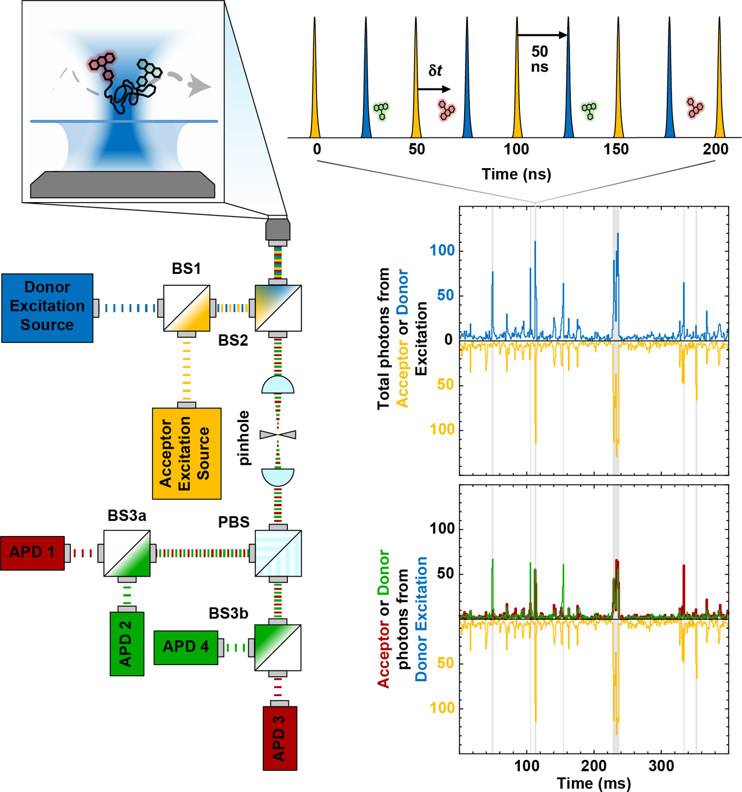
Two interleaved pulsed lasers (blue and yellow) for donor and acceptor excitation, respectively, are coaxially aligned using a dichroic mirror (BS1) and then directed into the back aperture of a high-numerical-aperture microscope objective. The spatial selection of the femtoliter confocal observation volume enables single-molecule detection at sub-nanomolar concentrations. When a single molecule diffuses through this volume, it produces a short (~1 ms) burst of donor (green) and acceptor (red) photons. The signal upon direct excitation of the acceptor is shown in yellow. Fluorescence photons are then collected by the same objective in an epifluorescence configuration, spatially separated from the excitation light using a second dichroic mirror (BS2), focused through a pinhole to reject out-of-focus fluorescence, split by polarization (PBS), and directed towards avalanche photodiodes (APDs 1–4) via a pair of dichroic mirrors (BS3a and BS3b) chosen to spectrally separate donor and acceptor fluorescence. The resulting four detection channels correspond to parallel and perpendicular polarized fluorescence from the donor and acceptor fluorophores, respectively.

Sample design and preparation

The success of any single-molecule FRET experiment is highly dependent on the design and quality of the sample. Essential design criteria are the spectral properties of the fluorophores and their Förster radius, which determines the accessible distance range, and the position of the dyes within the protein or nucleic acid. Over the last two decades, a preference has emerged for specific classes of fluorophores, primarily because of their commercial availability with versatile coupling chemistries, photostability, quantum yield, and compatibility with commonly available laser lines (Gust et al., 2014; Ha & Tinnefeld, 2012). Those two classes are rhodamine-based fluorophores (e.g., Alexa 488 as a donor and Alexa 594 as an acceptor), which are more commonly used for proteins, and cyanine-based fluorophores (e.g., Cy3 as a donor and Cy5 as an acceptor), which are more frequently used for nucleic acids. Additional considerations involve viable coupling chemistries, solvent exposure of the labeling sites, proximity to potential quenchers (e.g., other aromatic groups), and electrostatic interactions. Finally, the preparation and purification should minimize the amount of donor-only and acceptor-only contaminants within the FRET-labeled sample. For IDPs, this goal is most stringently achieved with high-resolution reversed-phase or ion exchange chromatography. Many of these issues have recently been discussed in detail elsewhere (Zosel, Holla, & Schuler, 2018).

Excitation scheme

A second important aspect for accurately determining transfer efficiencies in single-molecule FRET experiments is the excitation scheme (Fig. 1). In principle, it is possible to use a single laser to directly excite the donor fluorophore and then determine E from N_D and N_A. However, in practice, corrections for differences in quantum yields, detection efficiencies, spectral crosstalk, and direct excitation of the acceptor are required to accurately determine the transfer efficiency. A simple approach for obtaining these correction factors involves measurements of high concentrations of uncoupled fluorophores (Schuler, 2007), but it requires that the correction factors do not change upon coupling to the biomolecule, which is not always the case (Haenni, Zosel, Reymond, Nettels, & Schuler, 2013; Kretschy, Sack, & Somoza, 2016; Sanborn, Connolly, Gurunathan, & Levitus, 2007; Zosel, Haenni, Soranno, Nettels, & Schuler, 2017). This limitation can be circumvented by using an additional laser to alternatingly excite donor and acceptor fluorophores (Kapanidis et al., 2004; Muller, Zaychikov, Brauchle, & Lamb, 2005), which makes it possible to determine all correction factors directly from the labeled samples (Hellenkamp et al., 2018; Kudryavtsev et al., 2012; Lee et al., 2005). For this reason, most studies that aim to accurately measure single-molecule FRET efficiencies utilize some form of alternating excitation.

The basic idea behind this method is to alternate between donor and acceptor excitation and use time gating to analyze the photons from the two excitation sources separately. In practice, this can either be achieved using rapidly alternating continuous-wave lasers (referred to as Alternating Laser Excitation, ALEX)(Kapanidis et al., 2005; Kapanidis et al., 2004) or via interleaved pulsed lasers (referred to as Pulsed Interleaved Excitation, or PIE)(Kudryavtsev et al., 2012; Muller et al., 2005). Although the continuous-wave lasers used for ALEX often yield higher photon detection rates, the fluorescence lifetime information afforded by PIE is very useful for identifying undesired photophysical effects (e.g., quenching) or the presence of rapidly sampled distance distributions (see below). Therefore, this chapter will focus primarily on PIE (Fig. 1). However, apart from the lifetime information, the other aspects of PIE and ALEX are essentially identical with respect to instrument calibration.

Detection scheme

Another important aspect of any single-molecule FRET experiment is the detection system used for recording donor and acceptor fluorescence. Spectral separation of photons is easily achieved using dichroic mirrors, resulting in two detection channels: one for donor photons and another for acceptor photons. Additionally, it is useful to separate photons by polarization, resulting in four detection channels: donor parallel, donor perpendicular, acceptor parallel, and acceptor perpendicular (relative to the polarization of the excitation light). This four-channel approach provides access to information about the fluorescence anisotropy of the donor and acceptor, and, much like the lifetime data afforded by PIE, serves as an invaluable tool for identifying potential complications, especially hindered fluorophore rotation, that invalidate the basic assumptions necessary for quantitative transfer efficiency measurements (Sisamakis, Valeri, Kalinin, Rothwell, & Seidel, 2010). The detection scheme can be extended with additional spectral channels, e.g. to accommodate multi-color FRET, but here we focus on the commonly used and also commercially available (Wahl, Koberling, Patting, Rahn, & Erdmann, 2004) four-channel, two-color, configuration (Fig. 1).

Accurate FRET efficiencies

The value of E for each fluorescence burst in a free-diffusion measurement can be determined from the numbers of donor and acceptor photons after donor excitation. However, obtaining E experimentally is complicated by several effects: direct excitation of the acceptor fluorophore by the donor excitation source; leakage of donor emission into the acceptor detection channel; different quantum yields of donor and acceptor; different detection efficiencies for donor and acceptor photons; and background. These effects depend on many experimental factors, including the photophysical properties of the fluorophores; the excitation wavelengths and radiant fluxes; the combination of filters and dichroic mirrors associated with the detection system; the sensitivity of each detector; and the alignment of the instrument. Thus, even after correcting for background, we only obtain an apparent mean transfer efficiency, $\langle \widehat{E}\rangle =\langle \frac{{\widehat{N}}_A^d}{{\widehat{N}}_A^d+{\widehat{N}}_D^d}\rangle$, from the detected numbers of donor, ${\widehat{N}}_D^d$, and acceptor, ${\widehat{N}}_A^d$, photons in each burst. For the actual mean transfer efficiency, $\langle E\rangle =\langle \frac{N_A^d}{N_A^d+N_D^d}\rangle$, which is the desired quantity related to the distance between donor and acceptor via Eq. 3, we require the properly corrected values, $N_D^d$ and $N_A^d$. This section provides an overview of the analytical methods and workflow required to generate experimental correction factors from subpopulations of samples containing fluorescently labeled molecules (Hellenkamp et al., 2018; Kudryavtsev et al., 2012; Lee et al., 2005), which enable us to calculate $N_D^d$ and $N_A^d$ from ${\widehat{N}}_D^d$, and ${\widehat{N}}_A^d$.

Data analysis: Apparent fluorescence stoichiometry ratio and apparent FRET efficiency

One of the principle advantages of single-molecule experiments is their ability to separate individual subpopulations, provided that their photophysical properties are sufficiently different and their interconversion kinetics are slow relative to the burst duration. This is particularly obvious in PIE experiments that make use of both donor and acceptor excitation (Fig. 2). Such FRET measurements will typically be comprised of at least three distinct subpopulations: molecules that contain both an active donor and an active acceptor (‘FRET-active’), molecules with only active donor fluorophores (‘donor-only’), and molecules with only active acceptor fluorophores (‘acceptor-only’), where the latter two subpopulations almost inevitable arise from photobleaching and imperfectly labeled molecules.

Figure 2: Determining correction factors for acceptor direct excitation (δ) and donor cross talk (α).

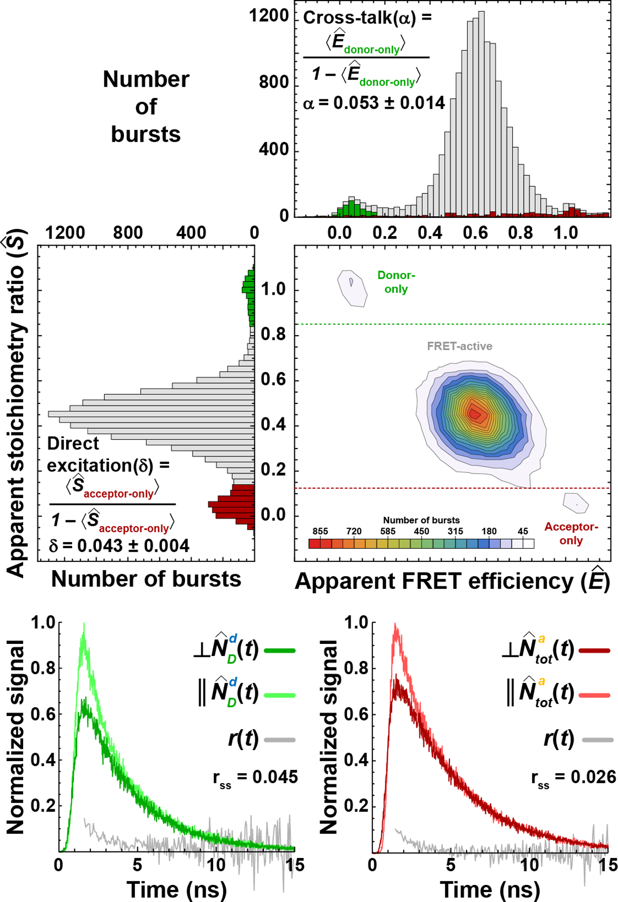
Using the apparent fluorescence stoichiometry ratio, $\widehat{S}$, it is possible to identify bursts from molecules with either only active donor (i.e., $\widehat{S}$ ≈ 1) or only active acceptor (i.e., $\widehat{S}$ ≈ 0) fluorophores. The apparent mean transfer efficiency, $\langle \widehat{E}\rangle$, of the donor-only subpopulation is used to determine the correction factor for cross-talk, $\alpha =\frac{\langle {\widehat{E}}_{\mathit{\text{donor}}-\mathit{\text{only}}}\rangle }{1-\langle {\widehat{E}}_{\mathit{\text{donor}}-\mathit{\text{only}}}\rangle }$. The apparent mean fluorescence stoichiometry ratio, $\langle \widehat{S}\rangle$, associated with the acceptor-only subpopulation is used to determine the correction factor for direct excitation, $\delta =\frac{\langle {\widehat{S}}_{\mathit{\text{acceptor}}-\mathit{\text{only}}}\rangle }{1-\langle {\widehat{S}}_{\mathit{\text{acceptor}}-\mathit{\text{only}}}\rangle }$ (due to background correction, Ê values for the acceptor-only bursts extend beyond the range shown). With pulsed interleaved excitation (PIE), time-correlated single-photon counting, and four-channel detection, it is also possible to obtain time-resolved fluorescence intensity and anisotropy decay plots from the parallel and perpendicular emission of the donor-only subpopulation after donor excitation (i.e., ∥ ${\widehat{N}}_D^d$ and ⊥ ${\widehat{N}}_D^d$) and the parallel and perpendicular emission of the acceptor-only subpopulations after acceptor excitation (i.e, ∥ ${\widehat{N}}_{tot}^a$ and ⊥ ${\widehat{N}}_{tot}^a$). This information is then used to determine the fluorescence lifetimes of donor and acceptor fluorophores and the time-resolved and the steady-state anisotropies (r_ss) of the fluorophores.

To separate these subpopulations, we utilize the total numbers of photons in a burst after donor excitation, $N_{tot}^d$, and acceptor excitation, $N_{tot}^a$, to define a parameter called the fluorescence stoichiometry ratio, $S=\frac{N_{tot}^d}{N_{tot}^d + N_{tot}^a}$. Bursts from FRET-active molecules are expected to have a stoichiometry ratio of S = ½, whereas donor-only and acceptor-only molecules should produce bursts of photons with S = 1, and S = 0, respectively. However, due to the previously mentioned complications associated with FRET measurements, the detected numbers of photons after donor excitation, ${\widehat{N}}_{tot}^d$, and acceptor excitation, ${\widehat{N}}_{tot}^a$, usually do not equal the values of $N_{tot}^d$ and $N_{tot}^a$. As a result, the mean apparent fluorescence stoichiometry ratio, $\langle \widehat{S}\rangle =\langle \frac{{\widehat{N}}_{tot}^d}{{\widehat{N}}_{tot}^d + {\widehat{N}}_{tot}^a}\rangle$, differs slightly from $\langle S\rangle =\langle \frac{N_{tot}^d}{N_{tot}^d + N_{tot}^a}\rangle$. Nevertheless, these three subpopulations can easily be identified via a histogram of $\widehat{S}$ and used to determine the correction factors needed for proper instrument calibration (Fig. 2).

Correction for cross-talk and acceptor direct excitation from donor-only and acceptor-only subpopulations

Donor-only molecules (i.e., $\widehat{S}$ ≈ 1) only emit donor photons and should thus ideally have an apparent mean transfer efficiency of $\langle {\widehat{E}}_{\mathit{\text{donor}}-\mathit{\text{only}}}\rangle =0$. However, due to spectral cross-talk, some donor photons leak into the acceptor detection channel, and as a result, $\langle {\widehat{E}}_{\mathit{\text{donor}}-\mathit{\text{only}}}\rangle >0$ (Fig 2). This non-zero value is used to define the cross-talk correction factor, $\alpha =\frac{\langle {\widehat{E}}_{\mathit{\text{donor}}-\mathit{\text{only}}}\rangle }{1-\langle {\widehat{E}}_{\mathit{\text{donor}}-\mathit{\text{only}}}\rangle }$. Similarly, acceptor-only molecules (i.e.,$\widehat{S}$ ≈ 0) do not contain a donor fluorophore and therefore should not be excited by the donor excitation laser. However, due to residual direct excitation of the acceptor fluorophore by the donor excitation laser, $\langle {\widehat{S}}_{\mathit{\text{acceptor}}-\mathit{\text{only}}}\rangle >0$ (Fig. 2). Again, this non-zero value is used to define the direct excitation correction factor, $\delta =\frac{\langle {\widehat{S}}_{\mathit{\text{acceptor}}-\mathit{\text{only}}}\rangle }{1-\langle {\widehat{S}}_{\mathit{\text{acceptor}}-\mathit{\text{only}}}\rangle }$. Then, α and δ are used to correct the detected number of acceptor photons after donor excitation for both cross-talk and direct excitation, $N_A^d={\widehat{N}}_A^d-\left(\alpha \cdot {\widehat{N}}_D^d\right)-\left(\delta \cdot {\widehat{N}}_{tot}^{ad}\right)$. Note that cross-talk of acceptor emission into the donor channel is usually negligible and can be ignored.

Correction for excitation and detection efficiencies from the FRET-active subpopulation

The values of $N_A^d$ are then used to redefine the apparent transfer efficiency and apparent fluorescence stoichiometry ratio of each burst:

$$\widehat{E}=\frac{N_A^d}{N_A^d+{\widehat{N}}_D^d}\text{\hspace{0.17em}\hspace{0.17em}\hspace{0.17em}and\hspace{0.17em}\hspace{0.17em}\hspace{0.17em}}\widehat{S}=\frac{N_A^d+{\widehat{N}}_D^d}{N_A^d+{\widehat{N}}_D^d+{\widehat{N}}_{tot}^a}.$$ (4)

Regardless of the $\langle \widehat{E}\rangle$ of a specific FRET-active subpopulation, it should have an apparent mean stoichiometry ratio of $\langle \widehat{S}\rangle$ = ½. However, because of the different excitation and detection efficiencies for the two fluorophores, this is generally not the case. Two additional correction factors account for these experimental imperfections. The relative excitation efficiency, β, describes how efficiently the two fluorophores are excited by their respective excitation lasers, $\beta =\left(P^a\cdot {\epsilon }_A^a\right)/\left(P^d\cdot {\epsilon }_D^d\right)$, where P^a and P^d represent the relative powers of the acceptor and donor excitation lasers, and ${\epsilon }_A^a$ and ${\epsilon }_D^d$ correspond to the extinction coefficients of the acceptor and donor fluorophores at their respective excitation wavelengths. The second correction factor, γ, accounts for the relative quantum yields and detection efficiencies for donor and acceptor emission, with γ = (ϕ_A·η_A)/(ϕ_D·η_D), where ϕ_A and ϕ_D are the quantum yields of donor and acceptor, and η_A and η_D are the detection efficiencies for donor and acceptor photons, respectively. The values of β and γ can be determined from the dependence of $\langle \widehat{S}\rangle$ on $\langle \widehat{E}\rangle$ using at least two subpopulations with different donor-acceptor distances (Lee et al., 2005):

$$\langle \widehat{S}\rangle \left(\langle \widehat{E}\rangle \right)=\frac{1}{1+\left(\beta \cdot \gamma \right)+\langle \widehat{E}\rangle \left(\beta -\left(\beta \cdot \gamma \right)\right)}$$ (5)

This relation shows that when γ = 1, $\langle \widehat{S}\rangle$ is independent of $\langle \widehat{E}\rangle$. If, additionally, the two fluorophores are excited with identical efficiency (i.e., β = 1), then $\langle \widehat{S}\rangle$ = ½. The factor γ is used to correct the number of donor photons detected after donor excitation for the different detection efficiencies of donor and acceptor photons (i.e., $N_D^d=\gamma \cdot {\widehat{N}}_D^d$), and the correction factor β is used to correct the total number of photons detected after acceptor excitation for the different excitation efficiencies of the two fluorophores (i.e., $N_{tot}^a=\frac{{\widehat{N}}_{tot}^a}{\beta }$). These two correction factors are then used to calculate the transfer efficiency, $E=\frac{N_A^d}{N_A^d+N_D^d}$, and stoichiometry ratio, $S=\frac{N_A^d+N_D^d}{N_A^d+N_D^d+N_{tot}^a}$, for each burst. The values of 〈S〉 and 〈E〉 can then be determined via a 2D-Gaussian fit to a plot of S vs. E for all FRET-active bursts of a given subpopulation. Because the correction factors γ and β are determined from the dependence of $\langle \widehat{S}\rangle$ on $\langle \widehat{E}\rangle$, we need to measure multiple subpopulations with different values of $\langle \widehat{E}\rangle$. This can be achieved in a variety of ways; the most straightforward is by working with a single sample with two or more well-separated subpopulations (e.g., native/denatured, bound/unbound, cis/trans, phosphorylated/dephosphorylated). However, it is often difficult to cleanly determine $\langle \widehat{S}\rangle$ and $\langle \widehat{E}\rangle$ when there are more than a few subpopulations in a single sample, which in turn limits the ability to determine β and γ. A more robust, albeit more time-consuming approach is to measure multiple independent samples (e.g., different biomolecules or different experimental conditions) labeled with the same fluorophores. Regardless of the approach, it is important to ensure that the differences in $\langle \widehat{E}\rangle$ arise solely because of different donor-acceptor distances and not because of differences in rotational flexibility, quenching of the fluorophores, changes in refractive index, or other effects that would lead to a change in R₀. It is thus important to quantify such contributions, e.g., for rotational motion via fluorescence anisotropies, for dynamic quenching via changes in fluorescence lifetimes, or for static quenching via nanosecond fluorescence correlation spectroscopy (Haenni et al., 2013; Zosel et al., 2017).

Calibration samples and measurements

To demonstrate this approach, we performed single-molecule FRET measurements of different IDPs and polyproline peptides labeled with Alexa 488 and Alexa 594 via maleimide chemistry (Fig. 3A). None of the samples showed detectable signs of hindered fluorophore rotation or quenching and yielded correction factors for acceptor direct excitation and donor cross-talk of α = 0.042 ± 0.014 and δ = 0.043 ± 0.004, respectively. These values were used to generate plots of $\widehat{S}$ vs. $\widehat{E}$ for each sample using Eq.4, with mean values determined from 2D-Gaussian fits. The resulting values of $\langle \widehat{S}\rangle$ and $\langle \widehat{E}\rangle$ were then analyzed with Eq. 5, yielding β = 1.16 ± 0.03 and γ = 1.27 ± 0.02 (Fig. 3A), which in turn were used to determine 〈S〉 and 〈E〉 for each of the eight samples (Fig. 3B). Once the correction factors are established for a given FRET pair and instrument configuration, they can be used for any future samples labeled with the same dyes, provided that the photophysical properties of the fluorophores do not differ from the reference samples. As recently demonstrated in a multi-laboratory benchmark study, this methodology typically results in transfer efficiencies with experimental uncertainties between ± 0.02 and ± 0.05 (Hellenkamp et al., 2018).

Figure 3: Quantifying correction factors for relative excitation (β) and detection (γ) efficiencies.

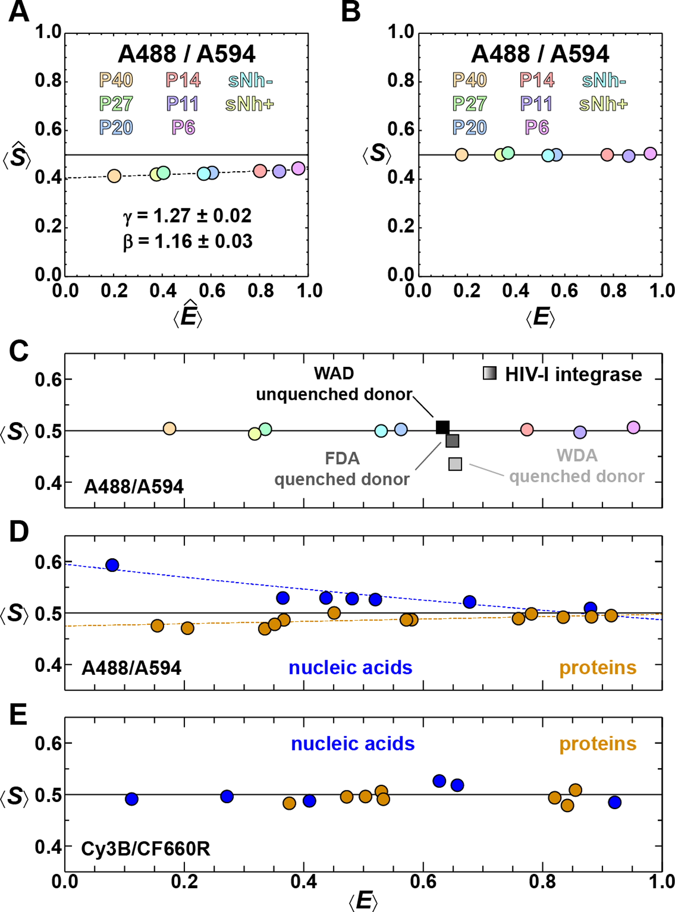
For each of the eight different samples, a 2D histogram of $\widehat{S}$ vs. $\widehat{E}$ is generated using Eq. 4 (Fig. 2) and the values of $\langle \widehat{S}\rangle$ and $\langle \widehat{E}\rangle$ for the FRET-active subpopulation of each sample determined using 2D-Gaussian fits. (A) These data are plotted and fit to Eq. 5 to determine the correction factors β and γ . (B) All four correction factors (i.e., α, δ, β, and γ) are then used to determine 〈S〉 and 〈E〉 for the eight samples (see Table 1). Note that 〈S〉 = ½ for all samples, independent of 〈E〉. (C) Species with photophysical irregularities can be identified via a deviation from 〈S〉 = ½, for example tryptophan-induced quenching of Alexa 488 in HIV-1 integrase (grey squares; see text for details). (D) Example of a set of correction factors derived from a collection of biomolecules labeled with Alexa 488/594 that results in 〈S〉 values that systematically deviate from ½, depending on the type of biomolecule. This deviation is quantified by fitting 〈S〉 vs. 〈E〉 for proteins and nucleic acids separately with Eq. 5 (colored dashed lines). This analysis indicates that the different local chemical environments of the fluorophores give rise to variations in their photophysical properties, resulting in different correction factors. (E) A more broadly applicable set of correction factors is obtained for another diverse set of proteins and nucleic acids labeled with Cy3B/CF660R, indicating that the photophysical properties of this FRET pair are less dependent on the local environment than those of the Alexa 488/594 FRET pair.

One of the advantages of determining 〈S〉 and 〈E〉 values for a larger sample set is that it is possible to identify cases where the photophysical properties (e.g., quantum yields) of the dyes deviate from the calibration set based on deviations from 〈S〉 = ½. To demonstrate this behavior, we use the N-terminal domain of HIV-1 integrase (IN), an IDP with a tryptophan residue at position 23 that is known to quench Alexa 488 (Zosel et al., 2017). The fluorescence stoichiometry ratio in the IN sample where Alexa 488 is close to the tryptophan residue (IN-WDA) deviates detectably from 〈S〉 = ½ (Fig. 3C), concomitant with a reduced donor fluorescence lifetime (Table 1). Replacing the tryptophan residue with phenylalanine (IN-FDA) shifts 〈S〉 closer to ½. Also, the donor lifetime determined from the donor-only population of IN-FDA is closer to the corresponding values of the calibration set, whose members lack any aromatic residues. A similar shift occurs when swapping the positions of the donor and acceptor (IN-WAD). This example illustrates that quenched samples can be identified based on the fluorescence stoichiometry ratio without having to directly monitor the fluorescence lifetime; the effects of quenching can then be taken into consideration when calculating 〈S〉 and 〈E〉 . The slight shift of IN-WAD to lower E, however, which is likely due to static quenching of the acceptor by the tryptophan (Haenni et al., 2013), is not obvious from this analysis and requires alternative methods for detection, such as nanosecond fluorescence correlation spectroscopy (Doose, Neuweiler, & Sauer, 2005; Haenni et al., 2013; Zosel et al., 2017).

Table1: Fluorescence parameters for IDP/polyproline samples.

Photophysical parameters: δ is the correction factor for acceptor direct excitation; τ_D is the donor-only fluorescence lifetime (from tail fits); α is the correction factor for spectral cross-talk; τ_A it the acceptor fluorescence lifetime (from tail fits); r_ss(donor) is the donor steady-state anisotropy of the donor-only subpopulation; and r_ss(acceptor) is the stead-state anisotropy of the acceptor-only subpopulation upon acceptor direct excitation. Note that δ increases upon coupling to proteins, an indication that the use of free dyes would result in non-representative correction factors. After the correction factors are applied, the mean fluorescence stoichiometry ratio of the reference data set is 〈S〉 = 0.501 ± 0.004. The decreased donor lifetimes of the HIV–1 Integrase sample result in a substantially decreased fluorescence stoichiometry ratio. Replacing the tryptophan near the donor fluorophore (IN-WDA) with a phenylalanine (IN-FDA) leads to an increase in donor lifetime and fluorescence stoichiometry ratio. A similar effect is apparent when the labeling positions of the donor and acceptor are swapped (IN-WAD). Color code as in Figure 4.

Sample		δ	τD	α	τA	rss(donor)	rss(acceptor)	〈E〉	〈S〉
Free-Dyes		0.035	3.92	0.041	3.89	*	*	-	-
Reference Data Set	P40	0.045	3.998	0.053	3.939	0.019	0.016	0.175	0.504
	P27	0.040	3.994	0.043	3.851	0.006	0.015	0.336	0.503
	P20	0.040	3.948	0.048	3.937	0.011	0.011	0.563	0.502
	P14	0.050	3.794	0.020	3.899	0.022	0.007	0.774	0.502
	P11	0.038	3.983	0.047	3.898	0.021	0.020	0.863	0.497
	P6	0.045	3.951	0.020	3.767	0.020	0.016	0.952	0.506
	sNh−	0.043	3.984	0.053	4.288	0.045	0.026	0.529	0.501
	sNh+	0.040	3.966	0.051	4.001	0.038	0.014	0.318	0.494
average		0.043	3.95	0.042	3.94	0.023	0.016	-	0.501
standard deviation		0.004	0.07	0.014	0.15	0.013	0.006	-	0.004
Integrase Data Set	IN-WDA	0.042	3.37	0.055	4.11	0.049	0.021	0.654	0.435
	IN-FDA	0.057	3.66	0.047	4.09	0.030	0.031	0.649	0.480
	IN-WAD	0.044	3.81	0.047	4.26	0.032	0.038	0.633	0.506

^*defined as zero for the purpose of correcting for differential collection efficiencies of the parallel and perpendicular detection channels

^-orange values in the Integrase Data Set are more than 3 standard deviations away from the mean of the Reference Data Set.

The photophysical parameters, and thus the correction factors, associated with the fluorophores can vary depending on the molecules they are coupled to. Therefore, we measured a diverse collection of FRET-labeled samples to determine how robust the correction factors are. This collection of molecules (Fig. 3D, E) is comprised of different types of biomolecules (folded proteins, intrinsically disordered proteins, as well as single- and double-stranded nucleic acids) labeled with two different FRET pairs (Cy3B/CF600R and Alexa 488/594) using different coupling chemistries (maleimide or N-succinimidyl ester). The molecules labeled with Alexa 488/594 exhibit significantly more scatter in 〈S〉 than the reference samples shown in Fig. 3C. Closer inspection reveals slightly but systematically different behavior for the nucleic acid and protein samples. Furthermore, the fluorescence stoichiometry ratios generated from this set are not independent of the transfer efficiency. These differences can be quantified by analyzing the protein and nucleic acid data points separately in the 〈S〉 vs. 〈E〉 plot (Fig. 3D) using Eq. 5, which results in γ′ = 0.65 ± 0.04 for nucleic acids and γ′ = 1.10 ± 0.04 for proteins. The significant deviations from the expected value of γ′ = 1 indicate that different correction factors should be used for the protein and nucleic acid samples with this dye pair. For instance, the error in the mean transfer efficiency of a protein sample at $\langle \widehat{E}\rangle$ = 0.5 analyzed using the correction factors from the nucleic acid samples would be $\Delta \langle E\rangle$ ≈ 0.14. However, this discrepancy is highly fluorophore-dependent: The data set in Fig. 3E for the Cy3B/CF600R FRET pair, e.g., yields correction factors (α = 0.038 ± 0.004, δ = 0.113 ± 0.007, β = 0.97 ± 0.03, γ = 0.60 ± 0.04 in this case) that are largely independent of the biomolecules the dyes are attached to.

The above examples (Fig. 3) illustrate how large sets of samples can provide robust correction factors necessary for accurate transfer efficiencies. These measurements can also reveal variability in the photophysical properties of fluorophores coupled to biomolecules. Both features make this approach ideally suited for quantifying distances in biomolecules, including IPDs.

Evidence for distance distributions from fluorescence lifetimes

Thus far, we have focused on obtaining accurate transfer efficiencies. The next step is to relate these values to the distances within the molecule. The key complication for IDPs is that they usually sample broad distance distributions, P(r), on a timescale much shorter than the microsecond interphoton times of typical single-molecule FRET experiments (Schuler, 2018; Schuler et al., 2016). If these conformational fluctuations occur on a timescale much longer than τ_D, then

$$\langle E\rangle =\langle \epsilon \rangle =\int P(r)\epsilon (r) dr.$$ (6)

Note that the mean values of ε and E are equal if the conformational dynamics occur between these two limiting timescales, but the distribution of E in a FRET efficiency histogram is determined primarily by shot noise arising from the 100 or so photons within each burst and not by the underlying P(r) that we would like to characterize.

However, in addition to 〈ε〉, it is possible to extract the variance, σ² = 〈ε²〉 − 〈ε〉², of the distribution of transfer efficiencies from single-molecule data acquired using PIE and time-correlated single-photon counting (Gopich & Szabo, 2012; Kalinin, Valeri, Antonik, Felekyan, & Seidel, 2010). The reason is that the relevant observation time in this case is the fluorescence lifetime, which is on the order of a few nanoseconds and thus much faster than the relaxation time of the inter-dye distance, which is typically in the range of tens to hundreds of nanoseconds for IDPs in the length range accessible to single-molecule FRET (Schuler, 2018; Schuler et al., 2016). To calculate σ², we estimate the donor fluorescence lifetime of each FRET-active burst, τ_DA, from the mean of the excitation-emission delay time, Δt_DA , of donor photons from the corresponding bursts, i.e., τ_DA = 〈Δt_DA〉. For a single fixed distance, 〈τ_DA〉/τ_D = 1 − ε, which follows directly from Eq. 2. However, since IDPs rapidly sample broad distance distributions, the value of τ_DA is biased towards longer times, because expanded conformations, for which the donor lifetime is longer, emit more donor photons than compact conformations. In a plot of τ_DA/τ_D vs. E (Fig. 4), this bias can be visualized as a displacement from the diagonal associated with a single fixed distance, also referred to as the ‘static FRET line’ (Kalinin et al., 2010). This displacement is then used to quantify σ² (Chung, Louis, & Gopich, 2016; Gopich & Szabo, 2012):

$$\frac{\langle {\tau }_{DA}\rangle }{{\tau }_D}=1 -\langle \epsilon \rangle +\frac{{\sigma }^2}{1-\langle \epsilon \rangle }$$ (7)

Correspondingly, bursts arising from molecules that have a broad but static transfer efficiency distribution (i.e., slow interconversion during the 1-ms burst duration), exemplified by the polyproline peptide shown in Fig. 4 (R. Best et al., 2007; Schuler, Lipman, Steinbach, Kumke, & Eaton, 2005), will cluster close to the diagonal, whereas intrinsically disordered proteins that dynamically sample a broad transfer efficiency distribution on the timescale of the interphoton time or faster, will cluster further above the diagonal. The lifetime information in these experiments can thus provide evidence for rapid conformational dynamics within a subpopulation. The experimental values of 〈ε〉 and σ² afford a model-independent assessment of P(r), and can in principle be used to parameterize the underlying distance distribution.

Figure 4: Assessing distributions of inter-dye distances with fluorescence lifetime information.

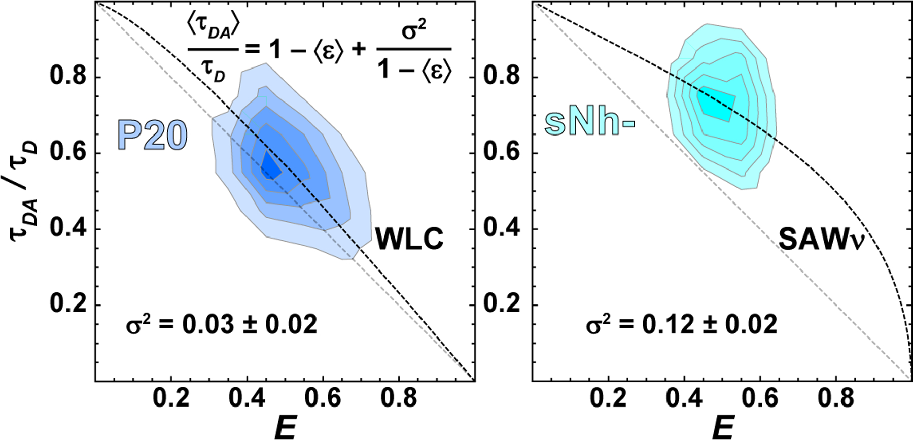
With pulsed interleaved excitation, it is possible to determine the relative donor lifetime in the presence of the acceptor, τ_DA/τ_D. This parameter provides information about the variance of the underlying distribution of transfer efficiencies. (left) In the case of a static distribution of distances in a 20-mer polyproline peptide (R. Best et al., 2007; Schuler et al., 2005), the values of 〈τ_DA〉/τ_D cluster close to the diagonal, which corresponds to a single fixed distance (static FRET line), 〈τ_DA〉/τ_D = 1 − ε. (right) However, for a broad and rapidly sampled distribution, for example the intrinsically disordered peptide sNh⁻, values of τ_DA/τ_D cluster above the diagonal. This vertical displacement provides a measure of the variance of the underlying distribution of transfer efficiencies, σ². In this way, lifetime vs. transfer efficiency plots can be used to assess the quality of polymer models (i.e., self-avoiding walk (Zheng et al., 2018), or worm-like chain (O’Brien, Morrison, Brooks, & Thirumalai, 2009)) commonly used to describe FRET-labeled biomolecules. The error of σ² was estimated assuming an uncertainty of ~0.1 ns for both τ_D and τ_DA.

Inferring distributions of distances and conformations

Thus far, we have discussed how the mean efficiency,〈ε〉, and its variance, σ², are related to an unspecified distribution, P(r), of the distance r between the chromophores. For folded proteins, the distance r usually fluctuates relatively little about its mean, so that a given 〈E〉 is commonly mapped directly to a mean distance via Eq. 3 (even though more quantitative approaches accounting for the flexibility of dye linkers are available (Kalinin et al., 2012; Muschielok et al., 2008)). Disordered and unfolded proteins, however, populate a very broad range of r. Therefore, it is necessary to characterize the distribution P(r) to obtain properties such as its mean and higher moments. In practice though, how can one reconstruct P(r) using the limited experimental information available? A reasonable choice, when it is safe to assume that the protein is disordered, is to take P(r) from a homopolymer model characterized by one or a small number of adjustable parameters that can be determined uniquely by fitting to the experimental data, so that the problem is well-posed. This is what is most commonly done for intrinsically disordered and unfolded proteins (Schuler et al., 2016), but some care is needed in order to obtain quantitatively accurate results (O’Brien et al., 2009), as we outline in section (i) below. In particular, it may be necessary to allow the form of P(r) to vary to accommodate changes in solution conditions (Zheng et al., 2018). In addition to inferring end-to-end distances, we would often like to know the radius of gyration $R_g=\frac{1}{2}{\left({\langle r_{ij}^2\left(m\right)\rangle }_{i,j,m}\right)}^{1/2}$ (here defined in terms of the average distances r_ij(m) over all atom pairs i, j, and also over all conformations m). This facilitates comparison with small-angle X-ray scattering, which measures R_g almost directly; R_g is also a fundamental property of interest of a disordered chain. However, FRET measures only P(r) for a single distance, and there is no fixed relationship between $R_g^2$ and 〈r²〉 – indeed it is known that the ratio of these quantities also varies with solution conditions (Borgia et al., 2016; Fuertes et al., 2017; Schäfer, 1999), which must be considered when interconverting them.

While analytical polymer models are by far the simplest to use, they can only be applied to single, fully disordered chains. Many proteins containing intrinsically disordered regions also contain folded domains (Oldfield & Dunker, 2014; van der Lee et al., 2014); others assemble into higher order complexes with other biomolecules (Wright & Dyson, 2015). Even among isolated disordered proteins, extreme variations of charge or hydrophobic patterning can cause deviations from the distributions that would be obtained from analytical homopolymer models (Das & Pappu, 2013; Fuertes et al., 2017). These more complex scenarios, which usually cannot be treated analytically and call for the use of molecular models, are the subject of sections (ii) and (iii). The chemical diversity inherent in disordered proteins means that it is also necessary to run molecular dynamics (or Monte Carlo) simulations of the molecular model in order to sample representative configurations of the system, which makes this procedure much more time consuming.

A further complication is that, unlike analytical polymer models, predictive simulation models typically have many parameters – how, then, should one adapt the model if it does not perfectly reproduce experiment? Bayesian statistics (or similarly, the maximum entropy principle), provides a solution in which the ensemble of structures obtained by simulation is minimally perturbed in order to match experiment. This is described in section (ii) below. An alternative scheme is to use a minimalist coarse-grained model, characterized by only a handful of free parameters. One may then fit the parameters of such a model directly to the data, as is described in section (iii). This “Occam’s Razor” approach avoids overfitting by using only a limited number of parameters in the model. In contrast, the Bayesian procedure in (ii) has many more parameters than can possibly be determined by the available data; it therefore requires a “regularization” procedure to avoid overfitting.

(i) Polymer model description of intrinsically disordered proteins.

Given a functional form for a distance distribution, P(r;a), characterized by parameter(s) a, one can straightforwardly determine a by numerically solving the integral equation (Eq. 6) above. A variety of models have been employed for this purpose, including the Gaussian chain, worm-like chain, and self-avoiding walk (Schuler et al., 2016). The distribution which has been most commonly used in the past is the Gaussian chain (GC). This is an idealized polymer in which the displacements between adjacent monomer units are governed by Gaussian statistics (a type of random walk), and there are no interactions between the monomer units (i.e., a “phantom chain”). The Gaussian chain P(r) is given by

$$P(r;R) ={\left(\frac{3}{2\pi }\right)}^{\frac{3}{2}}\frac{4\pi }{R}exp\left[-\frac{3}{2}{\left(\frac{r}{R}\right)}^2\right],$$ (8)

where the single parameter R is the root mean square end-to-end distance. One could then infer the radius of gyration by using the exact relation for a Gaussian chain, $R_g=R/\sqrt{6}$. This model is often a quite acceptable first approximation, in particular, since unfolded proteins in water are frequently close to the so-called theta state (Hofmann et al., 2012), in which protein-protein and protein-solvent interactions are balanced – the situation in which a Gaussian chain works best (Borgia et al., 2016; Zheng et al., 2018). However, where the protein interacts more favorably with the solvent than with itself (in high concentrations of chemical denaturant, or in a chain with high net charge, for example), a Gaussian chain tends to overestimate both the mean-square distance, as well as the inferred radius of gyration (Borgia et al., 2016; Fuertes et al., 2017; O’Brien et al., 2009; Song, Gomes, Gradinaru, & Chan, 2015). This overestimation arises from the neglect of excluded volume in a Gaussian chain, an effect that contributed partly to an apparent discrepancy between inferences of R_g from FRET and from small-angle X-ray scattering (SAXS) experiments (Yoo et al., 2012). This discrepancy has recently been resolved by improving the methods for analyzing both FRET and SAXS (Borgia et al., 2016; Fuertes et al., 2017; Riback et al., 2017; Zheng & Best, 2018; Zheng et al., 2018).

The end-to-end distance distribution when protein-solvent interactions are very favorable is better approximated by a self-avoiding walk (SAW), a model in which the residues in the protein have only short-range repulsive interactions between them. An approximation to the end-to-end distance distribution of the SAW is given by

$$P(r;R,\nu )=\frac{4\pi A}{R}{\left(\frac{r}{R}\right)}^{2+\frac{\gamma -1}{\nu }}exp\left[-\alpha {\left(\frac{r}{R}\right)}^{\frac{1}{1-\nu }}\right]$$ (9)

where R is the root mean square distance, γ ≈ 1.1615 is a critical exponent (Le Guillou & Zinn-Justin, 1977) and ν ≈ 0.6 is the Flory exponent for a self-avoiding walk. The constants A and α are determined from the requirements ${\int }_0^{\infty }P(r) \text{d}r=1$ and ${\int }_0^{\infty }P(r)r^2 \text{d}r=R^2$. For a SAW, $R_g=R\sqrt{6.26}$ for long chains. Examples of P(r) for a Gaussian chain and a self-avoiding walk corresponding to three different FRET efficiencies are given in Fig. 5. As is clear from the figure, it is possible to infer somewhat different average end-to-end distances from the same FRET efficiency when using different models; the change of the estimated average distance with FRET efficiency is also larger for the Gaussian chain. How can one minimize the model dependence of the inferred properties? Naively, one might assume that always using the same model to fit the FRET efficiency should give self-consistent results. Unfortunately, the most appropriate model depends on the effective solvent quality, which can vary with denaturant concentration, ionic strength, temperature, or amino acid sequence. In principle, it should be possible to use the additional information provided by σ² from fluorescence lifetime information (Fig. 4) to choose the most appropriate distribution. However, in practice, this variance is often very similar for the different models and does not have much discriminating power once the experimental error is considered. For example, in Fig. 5B at 〈ε〉 = 0.5, σ² is 0.13 for a GC and 0.11 for a SAW (see figure legend), whereas the intrinsically disordered peptide sNH⁻ in Fig. 4, which resides near 〈ε〉 = 0.5, has a variance of σ² = 0.12 ± 0.02 – i.e., the difference between the two models is within experimental error. Therefore, some additional information is needed to constrain the form of P(r). Furthermore, the Gaussian chain and self-avoiding walk represent two simplified limiting scenarios, while in reality a continuum of intermediate distributions is expected (for instance due to changes in solvent quality between theta solvent and good solvent for finite chains).

Figure 5. Illustration of the ambiguity in inferring a distance distribution from limited FRET data.

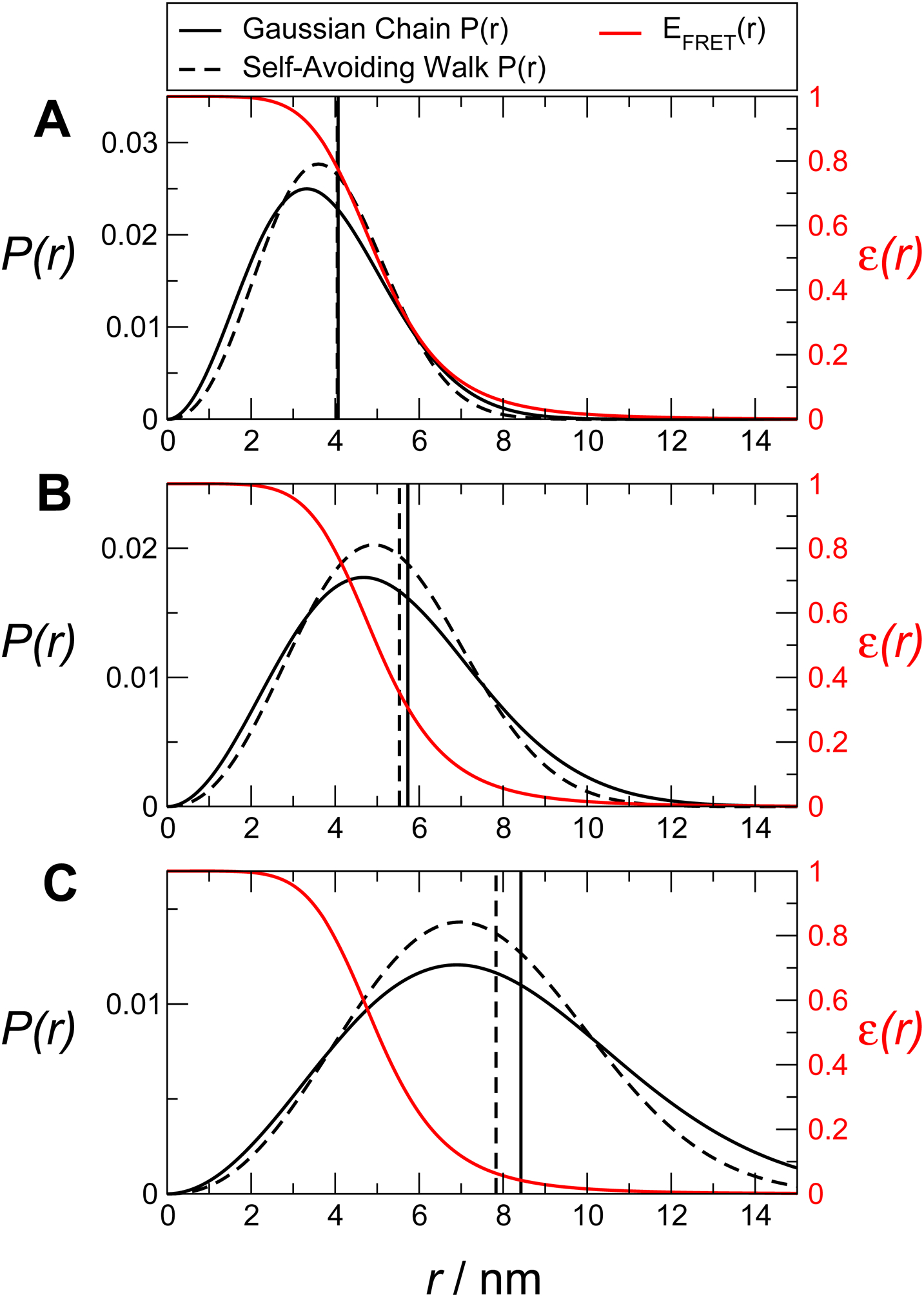
Distributions with mean efficiencies of 〈ε〉 = 0.75, 0.5, and 0.25 are shown in A, B, and C, respectively. In each case, the P(r) for a Gaussian chain and a self-avoiding walk corresponding to the same FRET efficiency are shown. The variances of the corresponding transfer efficiency distributions, σ², for the Gaussian chain and self-avoiding walk, respectively, are 0.08 and 0.07 in A, 0.13 and 0.11 in B, and 0.10 and 0.09 in C.

To overcome these difficulties, we recently proposed a semi-empirical approach, referred to as SAW-ν, in which the distance distribution is described via Eq. 9, but the exponent ν is treated as an adjustable parameter, rather than being fixed to 0.6 (Zheng et al., 2018). Consequently, two parameters, ν and R, must be determined, rather than one (R) for the GC or SAW. We have found that these parameters could not be reliably determined from the combination of 〈ε〉 and σ² readily available from FRET experiments (Zheng et al., 2018), because these parameters are highly correlated and σ² does not discriminate sufficiently between distributions, as discussed above. Instead, we use an approximate scaling law for the end-to-end distance in proteins to relate R to ν,

$$R=b{N}^{\nu },$$ (10)

in which the prefactor b is approximately 0.55 nm for proteins with well-mixed sequences (Hofmann et al., 2012) (for some low-complexity sequences or stiff homopolymers such as polyproline (Fig. 4A), a different prefactor may be required). This additional relation makes it possible to solve for the single free parameter characterizing the distribution, i.e., ν. In order to convert R² to $R_g^2$, we employ the approximate relation (Witten & Schäfer, 1978)

$$\frac{R^2}{R_g^2}=\frac{2(\gamma +2\nu )(\gamma +2\nu +1)}{\gamma (\gamma +1)}.$$ (11)

The SAW-ν model is thus able to interpolate between different forms of P(r), characterized by the scaling exponent ν. The quality of the fit can be tested against molecular simulation models, in which varying the temperature modulates the effective solvent quality, represented by ν. In Fig. 6, we apply the model to synthetic values of ε calculated from a simulation of a homopeptide (poly-Val) chain of length 100, at different temperatures (Fig. 6A). We can then use different models to attempt to reconstruct P(r) from the knowledge of the efficiencies only. Since we have data at multiple temperatures, we can see how well each model performs as a function of temperature, with each temperature corresponding to a different effective solvent quality.

Figure 6. Ability of polymer models to recover ensemble properties from simulation data.

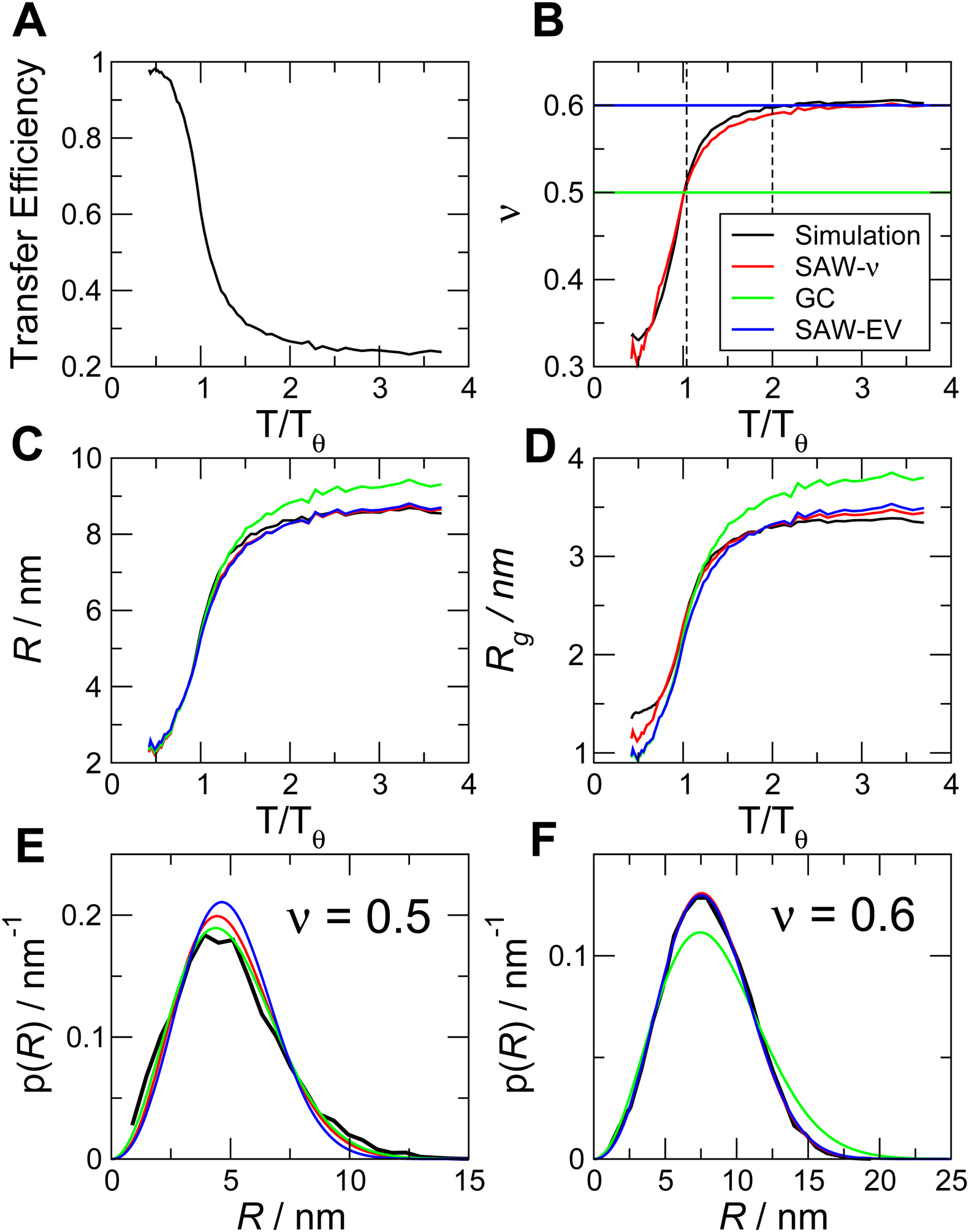
(A) Mean transfer efficiency computed from simulations of a simple homopolymer (Val₁₀₀), as a function of simulation temperature. (B) Scaling exponent ν computed directly from internal distance scaling (Borgia et al., 2016) in the simulation, and from the SAW-ν model (Zheng et al., 2018). Fixed ν implicit in Gaussian chain and SAW-EV models shown for reference (horizontal lines). Broken vertical lines indicate temperatures corresponding to ν ≈ 0.5 and ν ≈ 0.6 in (E) and (F). (C) End-to-end distance, R, and (D) radius of gyration, R_g, as a function of temperature, as calculated directly from the simulation, and as inferred from each polymer model (see legend in B). (E, F) P(r) at ν ≈ 0.5 and ν ≈ 0.6 respectively, as calculated directly from the simulation and as determined from fitting polymer models to the FRET efficiencies in (A).

We see that the SAW-ν can recover the scaling exponent ν computed directly from the protein coordinates in the simulations (Fig. 6B), while the Gaussian chain, or a self-avoiding walk with fixed ν=0.6 (SAW-EV) of course cannot capture this variation. Both SAW-ν and SAW-EV do a reasonable job of recovering the average end-to-end distance and radius of gyration (Fig. 6C, D). As noted above, the Gaussian chain tends to overestimate these quantities from the mean transfer efficiency when the chain is expanded. Looking in more detail at the distributions of end-to-end distance for simulations near the theta state (ν=0.5, Fig. 6E) and near the good solvent limit (ν=0.6, Fig. 6F), the Gaussian chain captures p(r) where ν=0.5, but is a poor approximation to the true distribution at ν=0.6. On the other hand, the SAW-EV model captures p(r) where ν = 0.6, but performs worst in capturing p(r) where ν = 0.5. These results simply reflect the relative strengths of each model discussed above. The SAW-ν model is able to fit both of these extreme scenarios similarly well. In summary, in the absence of additional information about the IDP of interest, the SAW-ν model is a good choice for approximating the underlying distance distributions.

Finally, to relate the experimentally observed average inter-dye distance to the distance between the two labeled residues, we need to account for the length of the dyes and linkers in this framework of analytical polymer models. The most common approach is to simply treat the dyes and linkers as part of the polymer chain and consider them equivalent to a suitably chosen number of amino acid residues. With the scaling exponent of the specific model used for the analysis (i.e., ν = 0.5 for GC, 0.6 for SAW-EV, or the respective value obtained with SAW-ν), the residue-residue distance is then estimated by rescaling the inter-dye distance via Eq. 10 and N=N_aa+L, where N is the sequence length of the interdye segment, comprising both the number of peptide bonds, N_aa, and the contribution from both dye linkers, L. The appropriate vale of L can be estimated, e.g., based on atomistic simulations (but the force field may need to be adjusted to prevent unrealistic dye sticking (R. B. Best, Hofmann, Nettels, & Schuler, 2015)). An experimental alternative is to infer it from a global analysis of a set of measurements of the same unfolded protein labeled at different sites, so that N_aa is known and different in every variant, but L is the same for all and can be treated as a fit parameter. For the Alexa 488/594 maleimide dye pair, e.g., such an analysis yielded L = 9 ± 2, corresponding to four or five residues per dye and linker (Aznauryan et al., 2016).

(ii) Combining experiment with simulations using Bayesian inference

An alternative to analytical polymer models for generating a distance distribution, P(r), is the use of molecular simulations. The advantage of such simulations is that, in addition to providing P(r), they also yield an ensemble of conformations, which we will denote {x_i}, that can be further analyzed. The protocol for running the simulations themselves is beyond the scope of this chapter to describe, but really any type of molecular representation can be used (e.g. from one bead per residue to all-atom), as long as the distance r in question can be computed from each conformation x_i. For the purposes of this section, we are thinking of simulations in which all atoms of the protein are explicitly represented. Such an ensemble allows additional details beyond P(r) to be determined, such as local secondary structure and the types of contacts that are formed most frequently. In an ideal world, a highly accurate, predictive simulation model would be used and the FRET data would merely be a check on the results. However, that level of accuracy is rarely achieved in practice, and the mean efficiency computed from the simulations will be somewhat different from experiment (Robert B. Best, Zheng, & Mittal, 2014). If the simulation model is a reasonably good approximation, and only a small shift in the distribution of configurations is needed, one might imagine reweighting the observed conformations x_i, each by a corresponding weight w_i, to give a reweighted efficiency

$${\langle \epsilon \rangle }_{\text{rw}}\left(\left\{w_i\right\}\right)=\sum _i{w}_i\epsilon (x_i)/\sum _i{w}_i.$$ (12)

In this expression, ε(x_i) is the FRET efficiency computed for conformation x_i. This can be optimized to match experiment by minimizing the χ² function, defined as

$${\chi }^2\left(\left\{w_i\right\}\right)=\sum _{k = 1}^{N_{obs}}\frac{{\left({\langle \epsilon \rangle }_{\text{rw}}\left(k;\left\{w_i\right\}\right)-{\langle \epsilon \rangle }_{expt}\left(k\right)\right)}^2}{\delta {\epsilon }^2\left(\text{k}\right)}.$$ (13)

Here, we describe the most general situation, in which several (N_obs) FRET efficiency observations are available, with the mean efficiency and experimental uncertainty of observation k (arising mostly from systematic calibration errors) given by 〈ε〉_expt(k) and δε(k), respectively. Multiple observed 〈ε〉expt(k) may come from different labeling positions of the protein (Borgia et al., 2016; Hoffmann et al., 2007), or from three-color FRET (Gambin & Deniz, 2010), but the procedure is still applicable even if only one observation is available. In the language of Bayesian statistics, minimizing χ² corresponds to maximizing the log-likelihood of the observed efficiencies, with a prior distribution given by the molecular simulation.

An obvious problem, considering the large and diverse ensemble of structures sampled in a typical simulation of a disordered protein, is that the solution {w_i} minimizing χ² is highly underdetermined by the data (Hummer & Koefinger, 2015). This difficulty may be overcome by requiring that the weights deviate minimally from the original (uniform) weights from the simulation. One way of achieving this is to introduce an additional term to the optimization function, penalizing sets of weights which differ from being uniform, and yielding the modified target function (Hummer & Koefinger, 2015)

$$\text{G}\left(\left\{w_i\right\}\right)={\chi }^2\left(\left\{w_i\right\}\right)-KS\left(\left\{w_i\right\}\right).$$ (14)

where the deviation from uniform weights is measured by the entropy of the weight set, $S={\sum }_i{w}_i\mathit{\text{ln\hspace{0.17em}}}{w}_i$. The factor K controls the relative importance of the penalty (or regularization) term. It is chosen to be as large as possible, thus keeping the weights as uniform as possible, without causing a large increase in χ². The weights are chosen using a Monte Carlo (MC) simulation, in which attempts to vary weights are accepted according to a Metropolis criterion (Borgia et al., 2016; Hummer & Koefinger, 2015). These simulations are run until χ² reaches a stable value. We note here that a similar formalism (Leung et al., 2016) was developed starting from the principal of maximum entropy (Jaynes, 1957), and has also been applied to refinement of disordered protein ensembles (Fuertes et al., 2017; Leung et al., 2016). Outside of the context of single-molecule FRET, a number of methods have been developed for ensemble refinement of proteins against experiment, as recently summarized in an excellent review (Bonomi, Heller, Camilloni, & Vendruscolo, 2017).

In Fig. 7, we show a practical example of this procedure, applied to FRET data from the intrinsically disordered protein ACTR as a function of denaturant concentration (Borgia et al., 2016). This data set includes FRET efficiencies for 3 different pairs of labeling positions of the protein under each set of conditions, which are combined in the ensemble fit (shown in Fig. 7A). In Fig. 7B, we show a plot of χ² vs S at each denaturant concentration. Different points on each curve correspond to different weight factors K. These curves show a plateau region at low χ² and low entropy, corresponding to smaller K. As K is increased, the entropy is increased, corresponding to more uniform sets of {w_i}, but this initially has little effect on χ², because there are many sets of {w_i} which can achieve this low χ². If K is increased too far, keeping the weights uniform becomes more important than reducing χ², and there is a sharp increase in χ². We chose the value of K immediately before this increase, as it corresponds to the highest entropy solution that is still able to fit the data (Borgia et al., 2016; Hummer & Koefinger, 2015; Mantsyzov et al., 2014). In 7A, we compare the experimentally observed efficiencies with the fits from the model with this optimal choice of K, and in Fig. 7C,D we show the average end-to-end distance, R, and R_g.

Figure 7. Bayesian ensemble reweighting of simulations of unfolded R17.

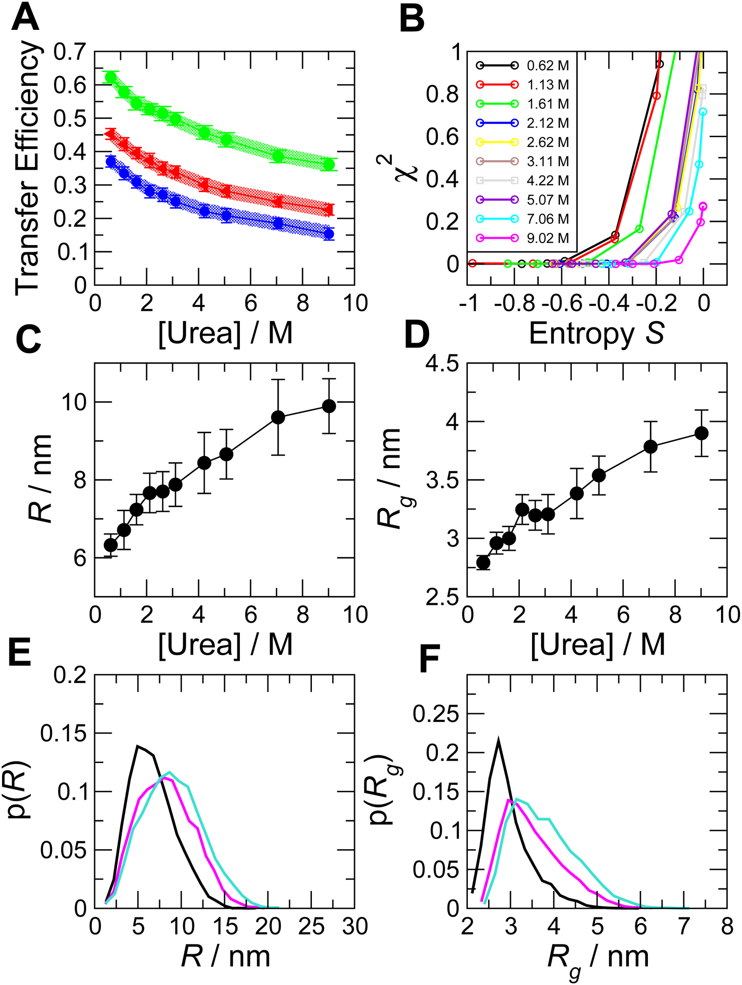
(A) FRET efficiency data versus denaturant concentration. Shaded regions show experimental confidence intervals (standard error), symbols and error bars show the values calculated from the reweighted ensemble. (B) Variation of χ² and S as the control parameter K is varied. Each curve corresponds to a given denaturant concentration (see legend) and each point to a particular value of K. Root mean square (C) distance, R, and (D) radius of gyration, R_g, are recovered as a function of denaturant. In (E) and (F) we show, respectively, examples of distribution functions for r and r_g (color code is: black, 1.13 M urea; magenta, 5.07 M urea; cyan, 9.02 M urea).

The penalty for non-uniform weights helps to avoid the solution being dominated by a few large weights w_i with the remainder being small. Nonetheless, a reweighting procedure of this sort always works best when there is good “overlap” between the initial ensemble of structures generated by the simulation and the final solution (i.e. weights are all approximately uniform)(Hummer & Koefinger, 2015). For example, if the initial distribution of conformations from simulation consisted almost entirely of compact structures, the only way to match experimental data reflecting an expanded distribution of conformations would be to have non-zero weights only for those few (if any) structures that are more expanded. Clearly this is undesirable when the underlying ensemble is expected to be a smooth distribution of diverse structures, not a few outliers, and this would be reflected in a lower entropy for the weights. One intuitive way of assessing this is to plot the distributions of various properties (e.g. R, R_g) from the initial, unweighted ensemble and also from the reweighted ensemble – it should not look like the reweighting is picking out only the tails of the distribution, and the reweighted distributions should (generally) look smooth, as illustrated for R and R_g in the example of ACTR introduced above (Fig. 7E,F). Another objective procedure is to compute the partition function for the weights, i.e. $Z=\left({\sum }_{i=1}^{N_s}{w}_i\right)/max\left[\left\{w_i\right\}\right]$, where N_S is the number of structures in the simulation ensemble. With this definition, the value of Z measures the number of structures contributing to the average. A good rule of thumb is that Z/N_S should be at least 0.2. In practice, there is no guarantee that a standard force field will have such a good overlap, therefore it is often helpful to generate a range of ensembles, for example at different simulation temperatures, and pick the temperature which yields the highest entropy fit or best overlap with the experimental data as the starting point for reweighting (Robert B. Best et al., 2018; Borgia et al., 2016).

An attractive feature of ensemble reweighting is that it is applicable to other types of experimental data besides FRET, as long as they can be computed from each structure in the ensemble. For example, we have recently applied it to joint refinement of unfolded state ensembles against FRET and SAXS data (Robert B. Best et al., 2018; Borgia et al., 2016). The main drawback is clearly that the procedure requires running a simulation of the system of interest, often several simulations under different conditions, in order to find one that overlaps well with the experimental data. In addition, some care is required in the reweighting procedure to avoid overfitting to a few structures. Therefore, if the protein in question can be described as a disordered chain, using a method such as SAW-ν to fit the data directly is a much easier alternative, but it cannot capture aspects such as secondary structure formation or other residue-specific interactions. Another advantage of detailed molecular simulations is that the fluorophores can be included explicitly if a suitable force field parametrization is available (R. B. Best et al., 2015; Zheng et al., 2016). Alternatively, rotamer libraries of fluorophores can be used to add the dyes after the simulation, albeit at the expense of information about their dynamics (Fuertes et al., 2017; Grotz et al., 2018).

(iii) Optimizing simulation parameters for simplified models

An alternative philosophy to the Bayesian reweighting scheme described above is a minimalist model. Rather than taking the view that atomistic simulations are a reasonable approximation needing only small improvements, one includes in the model only those features that are required to reproduce the experimental data, together with basic assumptions about protein structure that can be expected to be valid, such as covalent bonding between residues, and the size of a given residue type (Kim & Hummer, 2008; Tozzini, 2005). Such simplified models can potentially highlight which physical properties are most important for determining the observed conformational ensemble (i.e., properties that must be included in the model). The resulting model is naturally going to be quite coarse-grained, with little structural detail. An advantage, however, is that simulations of such models are much cheaper and faster to perform, and the energy landscape of the system is of lower dimensionality and smoother than those associated with all-atom simulations. Consequently, it is much easier to sample the system sufficiently to ensure that the results are independent of initial conditions (i.e. “converged” results), which is required for this method (it is desirable for Bayesian reweighting, but not absolutely essential in practice).

A typical minimalist model would represent each residue by a bead centered on its alpha carbon, with an energy function or force field, V_ff, of the form:

$$V_{ff}=V_{\mathit{\text{bonded}}}+\sum _{i<j}\frac{q_i{q}_j}{4\pi {ϵ}_{0}D}exp\left[-\frac{d_{ij}}{{\lambda }_D}\right]+\sum _{i<j}4e_{ij}\left({\left(\frac{s_{ij}}{r_{ij}}\right)}^{12}-{\left(\frac{s_{ij}}{r_{ij}}\right)}^6\right).$$ (15)

The first part of the energy, V_bonded, includes typical force field terms describing covalent bonding of the chain of residues, i.e. harmonic bond terms (or constraints), harmonic angle terms, and dihedral angle terms. These terms are described in more detail elsewhere (Borgia et al., 2018), and being transferable between different proteins, they would not generally be subject to optimization to fit experiment. The second term describes electrostatics in terms of a Debye-Hückel screening potential, with q_i being the charge on atom i, ϵ₀ the permittivity of free space, D the dielectric constant and λ_D the screening length. Being a physically-derived term, this is also not subject to optimization and is defined by the experimental ionic strength. The last term is the contact potential describing short-range interactions between the beads, here given in terms of a Lennard-Jones potential with contact distances s_ij between beads i and j and optimal interaction energies e_ij; r_ij is the distance between the beads. This is where the flexibility lies for fitting to experimental data. Although among the combinations of s_ij and e_ij there is in principle a large number of parameters, this can be greatly reduced. Firstly, the contact distances s_ij can be estimated from the known average volumes of different residue types in crystal structures (Kim & Hummer, 2008). The energies e_ij can be based on a standard contact potential for amino acids, such as the Miyazawa-Jernigan potential (Miyazawa & Jernigan, 1996). The simplest type of optimization would involve a global shifting and/or scaling of e_ij in the simulation in order to match the experimental transfer efficiency data. The optimal parameters can be obtained by a parameter search, most simply using a binary search in parameter space. Alternatively, a more sophisticated gradient-based parameter optimization could be used, as has recently been proposed for general force field refinement (Wang, Martinez, & Pande, 2014). The simplicity of the model allows multiple simulations with different parameters during optimization. A coarse-grained representation of the fluorophores and linkers can also be included in the model to assess their effect on the observed transfer efficiencies (Borgia et al., 2018).

Having given this very general outline of the form of the coarse-grained models used, we will illustrate the concept with the example of the binding of two highly charged proteins, prothymosin-α (ProTα) and histone H1 (H1) (Borgia et al., 2018). These are both intrinsically disordered proteins, except for the presence of a small folded domain in H1. The model used is similar to that given in Eq. 15 above, except for an extra term for the folded H1 domain, which is described in more detail by (Borgia et al., 2018); its purpose in this example is only to keep the domain folded throughout the simulation. The contact potential adopted is extremely simple, being just a single, common e_ij for all protein residue pairs, optimized against the single-molecule FRET data; more sophisticated potentials did not show better agreement with experiment. FRET efficiencies were measured for 28 inter- and intramolecular labeling pairs. Remarkably, it was possible to fit virtually all of the experimental FRET efficiencies, and in particular their pattern along the protein sequences (Fig. 8). From the resulting ensemble, we can compute the average distances between residue pairs, as well as distance distributions between any pair of residues of interest, some examples of which are shown also in Fig. 8. Lastly, one can go beyond distributions to characterize the ensemble of structures, a few of which are shown in Fig. 8. In this case, the simplicity of the energy function revealed that electrostatic interactions were the key factor in distinguishing the involvement of different regions of the protein sequence in the structure of the complex.

Figure 8: Fitting a coarse-grained model to experimental FRET efficiencies.

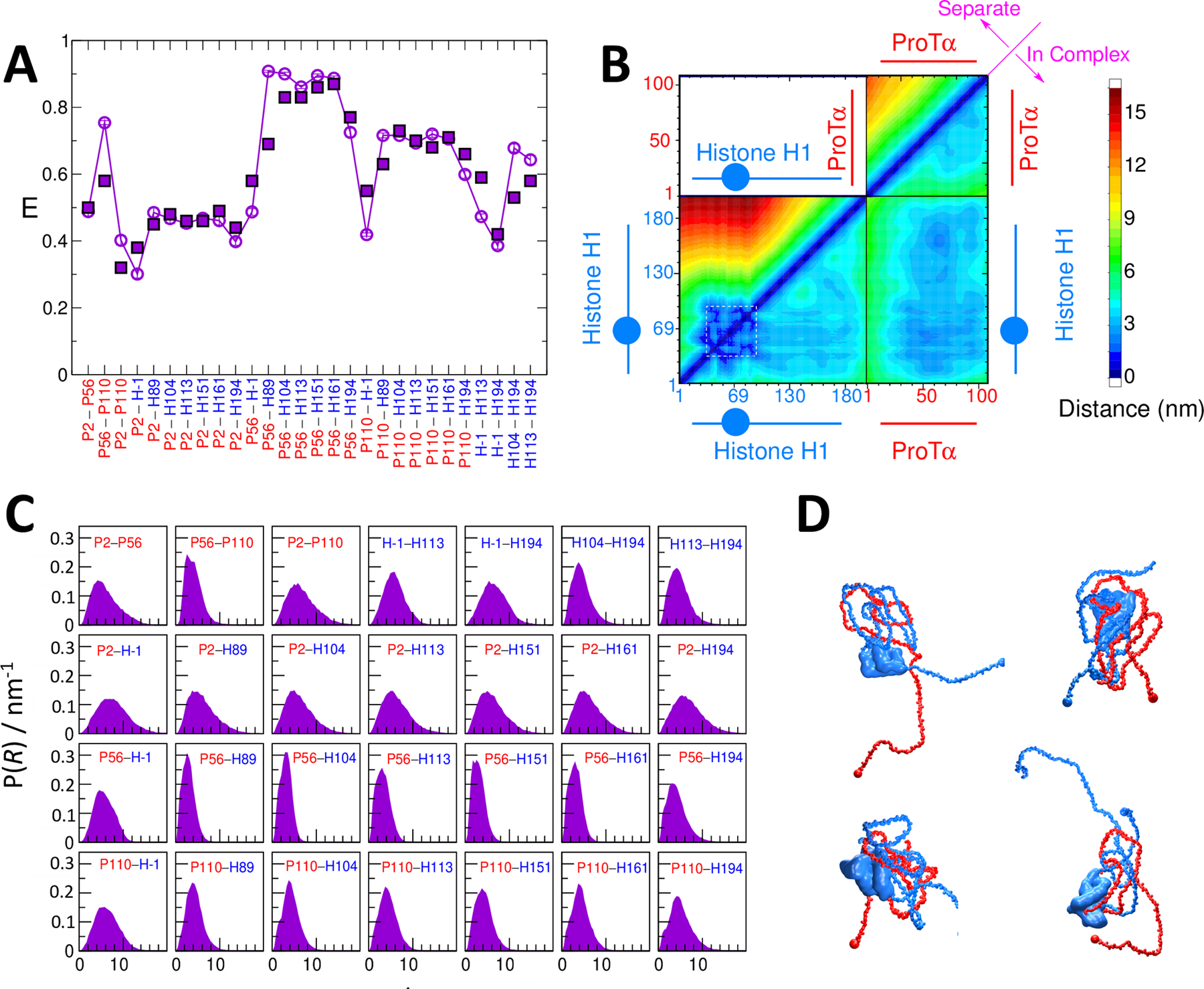
(A) Experimental (solid symbols) transfer efficiency data for inter- and intramolecular labeling pairs in the complex between ProTα and H1 (red: ProTα residue; blue: H1 residue). Empty symbols show results from the fitted model. (B) Average inter- and intramolecular pair distances between the two proteins. Blue circle in schematic of H1 represents the folded domain. (C) Pair distance distributions for labeled residue pairs from simulations with optimized energy function. (D) Example structures of ProTα-H1 complex.

Conclusions

Quantifying distances and distance distributions in IDPs with single-molecule FRET requires two key steps, which we have described here: (1) obtaining accurate transfer efficiencies, which rely on careful instrument calibration, and (2) extracting information about the structurally diverse ensemble of conformations based on a suitable model. Once accurate transfer efficiencies are available (ideally from multiple labeling positions), the simplest approach for inferring intramolecular distance distributions is the use of analytical polymer models, such as the SAW-ν model (Eq. 9), which often provides a good approximation. For a more detailed description that considers specific interactions, residual structure, or involves the complex of an IDP with a binding partner, the methods of choice are reweighting of molecular simulations or fitting of coarse-grained models to experimental data. These approaches further enable the direct integration with additional experimental results that afford complementary information, e.g. from NMR or scattering experiments. The resulting distance distributions can also be combined with nanosecond fluorescence correlation spectroscopy for quantifying intra- and interchain dynamics (Schuler, 2018). Single-molecule FRET thus increasingly contributes to our understanding of the structural, dynamic, and functional properties of IDPs.

References:

- Aznauryan M, Delgado L, Soranno A, Nettels D, Huang JR, Labhardt AM, et al. (2016). Comprehensive structural and dynamical view of an unfolded protein from the combination of single-molecule FRET, NMR, and SAXS. Proc. Natl. Acad. Sci. USA, 113(37), E5389–5398. doi: 10.1073/pnas.1607193113 [DOI] [PMC free article] [PubMed] [Google Scholar]
- Best R, Merchant K, Gopich IV, Schuler B, Bax A, & Eaton WA (2007). Effect of flexibility and cis residues in single molecule FRET studies of polyproline. Proc. Natl. Acad. Sci. USA, 104(48), 18964–18969 [DOI] [PMC free article] [PubMed] [Google Scholar]
- Best RB, Hofmann H, Nettels D, & Schuler B (2015). Quantitative Interpretation of FRET Experiments via Molecular Simulation: Force Field and Validation. Biophys J, 108(11), 2721–2731. doi: 10.1016/j.bpj.2015.04.038 [DOI] [PMC free article] [PubMed] [Google Scholar]
- Best RB, Zheng W, Borgia A, Buholzer K, Borgia MB, Hofmann H, et al. (2018). Comment on “Innovative scattering analysis shows that hydrophobic disordered proteins are expanded in water”. Science, 361, eaar7101 [DOI] [PMC free article] [PubMed] [Google Scholar]
- Best RB, Zheng W, & Mittal J (2014). Balanced protein-water interactions improve properties of disordered proteins and non-specific protein association. J. Chem. Theor. Comput, 10, 5113–5124 [DOI] [PMC free article] [PubMed] [Google Scholar]
- Bonomi M, Heller GT, Camilloni C, & Vendruscolo M (2017). Principles of protein structural ensemble determination. Curr Opin Struct Biol, 42, 106–116. doi: 10.1016/j.sbi.2016.12.004 [DOI] [PubMed] [Google Scholar]
- Borgia A, Borgia MB, Bugge K, Kissling VM, Heidarsson PO, Fernandes CB, et al. (2018). Extreme disorder in an ultrahigh-affinity protein complex. Nature, 555(7694), 61–66. doi: 10.1038/nature25762 [DOI] [PMC free article] [PubMed] [Google Scholar]
- Borgia A, Zheng W, Buholzer K, Borgia MB, Schuler A, Hofmann H, et al. (2016). Consistent View of Polypeptide Chain Expansion in Chemical Denaturants from Multiple Experimental Methods. J Am Chem Soc, 138(36), 11714–11726. doi: 10.1021/jacs.6b05917 [DOI] [PMC free article] [PubMed] [Google Scholar]
- Chung HS, Louis JM, & Gopich IV (2016). Analysis of Fluorescence Lifetime and Energy Transfer Efficiency in Single-Molecule Photon Trajectories of Fast-Folding Proteins. J Phys Chem B, 120(4), 680–699. doi: 10.1021/acs.jpcb.5b11351 [DOI] [PMC free article] [PubMed] [Google Scholar]
- Das RK, & Pappu RV (2013). Conformations of intrinsically disordered proteins are influenced by linear sequence distributions of oppositely charged residues. Proc Natl Acad Sci U S A, 110(33), 13392–13397. doi: 10.1073/pnas.1304749110 [DOI] [PMC free article] [PubMed] [Google Scholar]
- Deniz AA, Dahan M, Grunwell JR, Ha T, Faulhaber AE, Chemla DS, et al. (1999). Single-pair fluorescence resonance energy transfer on freely diffusing molecules: observation of Forster distance dependence and subpopulations. Proc Natl Acad Sci U S A, 96(7), 3670–3675 [DOI] [PMC free article] [PubMed] [Google Scholar]
- Deniz AA, Laurence TA, Dahan M, Chemla DS, Schultz PG, & Weiss S (2001). Ratiometric single-molecule studies of freely diffusing biomolecules. Annu. Rev. Phys. Chem, 52, 233–253 [DOI] [PubMed] [Google Scholar]
- Doose S, Neuweiler H, & Sauer M (2005). A close look at fluorescence quenching of organic dyes by tryptophan. Chemphyschem, 6(11), 2277–2285 [DOI] [PubMed] [Google Scholar]
- Dunker AK, Lawson JD, Brown CJ, Williams RM, Romero P, Oh JS, et al. (2001). Intrinsically disordered protein. J Mol Graph Model, 19(1), 26–59 [DOI] [PubMed] [Google Scholar]
- Dyson HJ, & Wright PE (2005). Intrinsically unstructured proteins and their functions. Nat Rev Mol Cell Biol, 6(3), 197–208. doi: 10.1038/nrm1589 [DOI] [PubMed] [Google Scholar]
- Ferreon AC, Moran CR, Gambin Y, & Deniz AA (2010). Single-molecule fluorescence studies of intrinsically disordered proteins. Methods Enzymol, 472, 179–204. doi: 10.1016/S0076-6879(10)72010-3 [DOI] [PubMed] [Google Scholar]
- Fischer E (1902). Nobel Lecture-Syntheses in the Purine and Sugar Group. Retrieved 29, May, 2018, from https://www.nobelprize.org/nobel_prizes/chemistry/laureates/1902/fischer-lecture.pdf
- Forman-Kay JD, & Mittag T (2013). From sequence and forces to structure, function, and evolution of intrinsically disordered proteins. Structure, 21(9), 1492–1499. doi: 10.1016/j.str.2013.08.001 [DOI] [PMC free article] [PubMed] [Google Scholar]
- Förster T (1948). Zwischenmolekulare Energiewanderung Und Fluoreszenz. Annalen der Physik, 2(1–2), 55–75 [Google Scholar]
- Fuertes G, Banterlea N, Ruff KM, Chowdhury A, Mercadante D, Koehler C, et al. (2017). Decoupling of size and shape fluctuations in heteropolymeric sequences reconciles discrepancies in SAXS vs. FRET measurements. Proceedings of the National Academy of Sciences of the United States of America, 114(31), E6342–E6351. doi: 10.1073/pnas.1704692114 [DOI] [PMC free article] [PubMed] [Google Scholar]
- Gambin Y, & Deniz AA (2010). Multicolor single-molecule FRET to explore protein folding and binding. Mol Biosyst, 6(9), 1540–1547. doi: 10.1039/c003024d [DOI] [PMC free article] [PubMed] [Google Scholar]
- Gibbs EB, & Showalter SA (2015). Quantitative biophysical characterization of intrinsically disordered proteins. Biochemistry, 54(6), 1314–1326. doi: 10.1021/bi501460a [DOI] [PubMed] [Google Scholar]
- Gomes GN, & Gradinaru CC (2017). Insights into the conformations and dynamics of intrinsically disordered proteins using single-molecule fluorescence. Biochim Biophys Acta, 1865(11 Pt B), 1696–1706. doi: 10.1016/j.bbapap.2017.06.008 [DOI] [PubMed] [Google Scholar]
- Gopich IV, & Szabo A (2012). Theory of the energy transfer efficiency and fluorescence lifetime distribution in single-molecule FRET. Proc Natl Acad Sci U S A, 109(20), 7747–7752. doi: 10.1073/pnas.1205120109 [DOI] [PMC free article] [PubMed] [Google Scholar]
- Grotz KK, Nüesch M, Holmstrom E, Heinz M, Stelzl LS, Schuler B, et al. (2018). Dispersion Correction Alleviates Dye Stacking of Single-Stranded DNA and RNA in Simulations of Single-Molecule Fluorescence Experiments. J. Phys. Chem. B, under revision [DOI] [PubMed] [Google Scholar]
- Gust A, Zander A, Gietl A, Holzmeister P, Schulz S, Lalkens B, et al. (2014). A starting point for fluorescence-based single-molecule measurements in biomolecular research. Molecules, 19(10), 15824–15865. doi: 10.3390/molecules191015824 [DOI] [PMC free article] [PubMed] [Google Scholar]
- Ha T, & Tinnefeld P (2012). Photophysics of fluorescent probes for single-molecule biophysics and super-resolution imaging. Annu Rev Phys Chem, 63, 595–617. doi: 10.1146/annurev-physchem-032210-103340 [DOI] [PMC free article] [PubMed] [Google Scholar]
- Haenni D, Zosel F, Reymond L, Nettels D, & Schuler B (2013). Intramolecular distances and dynamics from the combined photon statistics of single-molecule FRET and photoinduced electron transfer. J Phys Chem B, 117(42), 13015–13028. doi: 10.1021/jp402352s [DOI] [PubMed] [Google Scholar]
- Hellenkamp B, Schmid S, Doroshenko O, Opanasyuk O, Kühnemuth R, Adariani SR, et al. (2018). Precision and accuracy of single-molecule FRET measurements - a worldwide benchmark study. Nature Methods, 15(15), 669–676 [DOI] [PMC free article] [PubMed] [Google Scholar]
- Hellenkamp B, Wortmann P, Kandzia F, Zacharias M, & Hugel T (2017). Multidomain structure and correlated dynamics determined by self-consistent FRET networks. Nat Methods, 14(2), 174–180. doi: 10.1038/nmeth.4081 [DOI] [PMC free article] [PubMed] [Google Scholar]
- Hoffmann A, Kane A, Nettels D, Hertzog DE, Baumgärtel P, Lengefeld J, et al. (2007). Mapping protein collapse with single-molecule fluorescence and kinetic synchrotron radiation circular dichroism spectroscopy. Proc. Natl. Acad. Sci. USA, 104(1), 105–110 [DOI] [PMC free article] [PubMed] [Google Scholar]
- Hofmann H, Soranno A, Borgia A, Gast K, Nettels D, & Schuler B (2012). Polymer scaling laws of unfolded and intrinsically disordered proteins quantified with single-molecule spectroscopy. Proc Natl Acad Sci U S A, 109(40), 16155–16160. doi: 10.1073/pnas.1207719109 [DOI] [PMC free article] [PubMed] [Google Scholar]
- Hummer G, & Koefinger J (2015). Bayesian ensemble refinement by replica simulations and reweighting. Journal of Chemical Physics, 143(24). doi:Artn 243150 10.1063/1.4937786 [DOI] [PubMed] [Google Scholar]
- Jaynes ET (1957). Information theory and statistical mechanics. Phys. Rev , 106, 620–630 [Google Scholar]
- Kalinin S, Peulen T, Sindbert S, Rothwell PJ, Berger S, Restle T, et al. (2012). A toolkit and benchmark study for FRET-restrained high-precision structural modeling. Nat Methods, 9(12), 1218–1225. doi: 10.1038/nmeth.2222 [DOI] [PubMed] [Google Scholar]
- Kalinin S, Valeri A, Antonik M, Felekyan S, & Seidel CA (2010). Detection of structural dynamics by FRET: a photon distribution and fluorescence lifetime analysis of systems with multiple states. [Research Support, Non-U.S. Gov’t]. J. Phys. Chem. B, 114(23), 7983–7995. doi: 10.1021/jp102156t [DOI] [PubMed] [Google Scholar]
- Kapanidis AN, Laurence TA, Lee NK, Margeat E, Kong X, & Weiss S (2005). Alternating-laser excitation of single molecules. Acc Chem Res, 38(7), 523–533. doi: 10.1021/ar0401348 [DOI] [PubMed] [Google Scholar]
- Kapanidis AN, Lee NK, Laurence TA, Doose S, Margeat E, & Weiss S (2004). Fluorescence-aided molecule sorting: analysis of structure and interactions by alternating-laser excitation of single molecules. Proc Natl Acad Sci U S A, 101(24), 8936–8941. doi: 10.1073/pnas.0401690101 [DOI] [PMC free article] [PubMed] [Google Scholar]
- Kikhney AG, & Svergun DI (2015). A practical guide to small angle X-ray scattering (SAXS) of flexible and intrinsically disordered proteins. FEBS Lett, 589(19 Pt A), 2570–2577. doi: 10.1016/j.febslet.2015.08.027 [DOI] [PubMed] [Google Scholar]
- Kim YC, & Hummer G (2008). Coarse-grained models for simulations of multiprotein complexes: application to ubiquitin binding. J. Mol. Biol, 375, 1416–1433 [DOI] [PMC free article] [PubMed] [Google Scholar]
- König I, Zarrine-Afsar A, Aznauryan M, Soranno A, Wunderlich B, Dingfelder F, et al. (2015). Single-molecule spectroscopy of protein conformational dynamics in live eukaryotic cells. Nat Methods, 12(8), 773–779. doi: 10.1038/nmeth.3475 [DOI] [PubMed] [Google Scholar]
- Konrat R (2014). NMR contributions to structural dynamics studies of intrinsically disordered proteins. J Magn Reson, 241, 74–85. doi: 10.1016/j.jmr.2013.11.011 [DOI] [PMC free article] [PubMed] [Google Scholar]
- Kretschy N, Sack M, & Somoza MM (2016). Sequence-Dependent Fluorescence of Cy3- and Cy5-Labeled Double-Stranded DNA. Bioconjug Chem, 27(3), 840–848. doi: 10.1021/acs.bioconjchem.6b00053 [DOI] [PMC free article] [PubMed] [Google Scholar]
- Kudryavtsev V, Sikor M, Kalinin S, Mokranjac D, Seidel CA, & Lamb DC (2012). Combining MFD and PIE for accurate single-pair Forster resonance energy transfer measurements. Chemphyschem, 13(4), 1060–1078. doi: 10.1002/cphc.201100822 [DOI] [PubMed] [Google Scholar]
- Le Guillou JC, & Zinn-Justin J (1977). Critical Exponents for N-Vector Model in 3 Dimensions from Field-Theory. Physical Review Letters, 39(2), 95–98. doi:Doi 10.1103/Physrevlett.39.95 [DOI] [Google Scholar]
- Lee NK, Kapanidis AN, Wang Y, Michalet X, Mukhopadhyay J, Ebright RH, et al. (2005). Accurate FRET measurements within single diffusing biomolecules using alternating-laser excitation. Biophys J, 88(4), 2939–2953. doi: 10.1529/biophysj.104.054114 [DOI] [PMC free article] [PubMed] [Google Scholar]
- Leung HTA, Bignucolo O, Aregger R, Dames SA, Mazur A, Bernèche S, et al. (2016). A rigorous and efficient method to reweight very large conformational ensembles using average experimental data and to determine their relative information content. J. Chem. Theor. Comput, 12, 383–394 [DOI] [PubMed] [Google Scholar]
- Mantsyzov AB, Maltsev AS, Ying J, Shen Y, Hummer G, & Bax A (2014). A maximum entropy approach to the study of residue-specific backbone angle distributions in alpha-synuclein, an intrinsically disordered protein. Protein Sci, 23, 1275–1290 [DOI] [PMC free article] [PubMed] [Google Scholar]
- Miyazawa S, & Jernigan RL (1996). Residue-residue potentials with a favourable contact pair term and an unfavourable high packing density term, for simulation and threading. J. Mol. Biol, 256, 623–644 [DOI] [PubMed] [Google Scholar]
- Muller BK, Zaychikov E, Brauchle C, & Lamb DC (2005). Pulsed interleaved excitation. Biophys J, 89(5), 3508–3522. doi: 10.1529/biophysj.105.064766 [DOI] [PMC free article] [PubMed] [Google Scholar]
- Muschielok A, Andrecka J, Jawhari A, Bruckner F, Cramer P, & Michaelis J (2008). A nano-positioning system for macromolecular structural analysis. Nat Methods, 5(11), 965–971. doi: 10.1038/nmeth.1259 [DOI] [PubMed] [Google Scholar]
- O’Brien EP, Morrison G, Brooks BR, & Thirumalai D (2009). How accurate are polymer models in the analysis of Forster resonance energy transfer experiments on proteins? J Chem Phys, 130(12), 124903. doi: 10.1063/1.3082151 [DOI] [PMC free article] [PubMed] [Google Scholar]
- Oates ME, Romero P, Ishida T, Ghalwash M, Mizianty MJ, Xue B, et al. (2013). D(2)P(2): database of disordered protein predictions. Nucleic Acids Res, 41(Database issue), D508–516. doi: 10.1093/nar/gks1226 [DOI] [PMC free article] [PubMed] [Google Scholar]
- Oldfield CJ, & Dunker AK (2014). Intrinsically disordered proteins and intrinsically disordered protein regions. Annu. Rev. Biochem, 83, 553–584 [DOI] [PubMed] [Google Scholar]
- Riback JA, Bowman MA, Zmyslowski AM, Knoverek CR, Jumper JM, Hinshaw JR, et al. (2017). Innovative scattering analysis shows that hydrophobic disordered proteins are expanded in water. Science, 358(6360), 238–241. doi: 10.1126/science.aan5774 [DOI] [PMC free article] [PubMed] [Google Scholar]
- Sanborn ME, Connolly BK, Gurunathan K, & Levitus M (2007). Fluorescence properties and photophysics of the sulfoindocyanine Cy3 linked covalently to DNA. J Phys Chem B, 111(37), 11064–11074. doi: 10.1021/jp072912u [DOI] [PubMed] [Google Scholar]
- Schäfer L (1999). Excluded Volume Effects in Polymer Solutions as Explained by the Renormalization Group. Berlin: Springer. [Google Scholar]
- Schuler B (2007). Application of single molecule Forster resonance energy transfer to protein folding. Methods Mol Biol, 350, 115–138 [DOI] [PubMed] [Google Scholar]
- Schuler B (2018). Perspective: Chain dynamics of unfolded and intrinsically disordered proteins from nanosecond fluorescence correlation spectroscopy combined with single-molecule FRET. J. Chem. Phys, 149(1), 010901. [DOI] [PubMed] [Google Scholar]
- Schuler B, & Hofmann H (2013). Single-molecule spectroscopy of protein folding dynamics--expanding scope and timescales. Curr Opin Struct Biol, 23(1), 36–47. doi: 10.1016/j.sbi.2012.10.008 [DOI] [PubMed] [Google Scholar]
- Schuler B, Lipman EA, Steinbach PJ, Kumke M, & Eaton WA (2005). Polyproline and the “spectroscopic ruler” revisited with single molecule fluorescence. Proc. Natl. Acad. Sci. USA, 102, 2754–2759 [DOI] [PMC free article] [PubMed] [Google Scholar]
- Schuler B, Soranno A, Hofmann H, & Nettels D (2016). Single-Molecule FRET Spectroscopy and the Polymer Physics of Unfolded and Intrinsically Disordered Proteins. Annu Rev Biophys, 45, 207–231. doi: 10.1146/annurev-biophys-062215-010915 [DOI] [PubMed] [Google Scholar]
- Sisamakis E, Valeri A, Kalinin S, Rothwell PJ, & Seidel CAM (2010). Accurate Single-Molecule FRET Studies Using Multiparameter Fluorescence Detection. Methods Enzymol, 475, 455–514 [DOI] [PubMed] [Google Scholar]
- Song J, Gomes G-N, Gradinaru C, & Chan HS (2015). An adequate account of excluded volume Is necessary to infer compactness and asphericity of disordered proteins by Förster resonance energy transfer. J. Phys. Chem. B, 119, 15191–15202 [DOI] [PubMed] [Google Scholar]
- Stryer L (1978). Fluorescence energy transfer as a spectroscopic ruler. Annu Rev Biochem, 47, 819–846. doi: 10.1146/annurev.bi.47.070178.004131 [DOI] [PubMed] [Google Scholar]
- Stryer L, & Haugland RP (1967). Energy transfer: a spectroscopic ruler. Proc Natl Acad Sci U S A, 58(2), 719–726 [DOI] [PMC free article] [PubMed] [Google Scholar]
- Sustarsic M, & Kapanidis AN (2015). Taking the ruler to the jungle: single-molecule FRET for understanding biomolecular structure and dynamics in live cells. Curr Opin Struct Biol, 34, 52–59. doi: 10.1016/j.sbi.2015.07.001 [DOI] [PubMed] [Google Scholar]
- Tompa P (2005). The interplay between structure and function in intrinsically unstructured proteins. FEBS Lett, 579(15), 3346–3354. doi: 10.1016/j.febslet.2005.03.072 [DOI] [PubMed] [Google Scholar]
- Tozzini V (2005). Coarse-grained models for proteins. Curr. Opin. Struct. Biol, 15, 144–150 [DOI] [PubMed] [Google Scholar]
- Uversky V. N. a. D. AK (Ed.). (2012). Intrinsically Disordered Protein Analysis (Vol. 896). New York: Springer. [Google Scholar]
- van der Lee R, Buljan M, Lang B, Weatheritt RJ, Daughdrill GW, Dunker AK, et al. (2014). Classification of intrinsically disordered regions and proteins. Chem Rev, 114(13), 6589–6631. doi: 10.1021/cr400525m [DOI] [PMC free article] [PubMed] [Google Scholar]
- Van Der Meer BW, Coker G III, Chen SYS (1994). Resonance energy transfer: theory and data. New York: VCH Publishers, Inc. [Google Scholar]
- Wahl M, Koberling F, Patting M, Rahn H, & Erdmann R (2004). Time-resolved confocal fluorescence imaging and spectrocopy system with single molecule sensitivity and sub-micrometer resolution. Curr. Pharm. Biotechnol, 5(3), 299–308 [DOI] [PubMed] [Google Scholar]
- Wang L-P, Martinez TJ, & Pande VS (2014). Building force fields: an automatic, systematic and reproducible approach. J. Chem. Theor. Comput, 5, 1885–1891 [DOI] [PMC free article] [PubMed] [Google Scholar]
- Witten TA, & Schäfer L (1978). Two critical ratios in polymer solutions. J. Phys. A, 11(9), 1843–1854 [Google Scholar]
- Wright PE, & Dyson HJ (2015). Intrinsically disordered proteins in cellular signalling and regulation. Nat. Rev. Mol. Cell Biol, 16, 18–29 [DOI] [PMC free article] [PubMed] [Google Scholar]
- Yoo TY, Meisberger SP, Hinshaw J, Pollack L, Haran G, Sosnick TR, et al. (2012). Small-angle X-ray scattering and single-molecule FRET spectroscopy produce highly divergent views of the low-denaturant unfolded state. J. Mol. Biol, 418, 226–236 [DOI] [PMC free article] [PubMed] [Google Scholar]
- Zheng W, & Best RB (2018). An extended Guinier analysis for intrinsically disordered proteins. J. Mol. Biol, 430, 2540–2553 [DOI] [PMC free article] [PubMed] [Google Scholar]
- Zheng W, Borgia A, Buholzer K, Grishaev A, Schuler B, & Best RB (2016). Probing the Action of Chemical Denaturant on an Intrinsically Disordered Protein by Simulation and Experiment. J. Am. Chem. Soc, 138(36), 11702–11713. doi: 10.1021/jacs.6b05443 [DOI] [PMC free article] [PubMed] [Google Scholar]
- Zheng W, Zerze GH, Borgia A, Mittal J, Schuler B, & Best RB (2018). Inferring properties of disordered chains from FRET transfer efficiencies. J Chem Phys, 148(12), 123329. doi: 10.1063/1.5006954 [DOI] [PMC free article] [PubMed] [Google Scholar]
- Zosel F, Haenni D, Soranno A, Nettels D, & Schuler B (2017). Combining short- and long-range fluorescence reporters with simulations to explore the intramolecular dynamics of an intrinsically disordered protein. J Chem Phys, 147(15), 152708. doi: 10.1063/1.4992800 [DOI] [PubMed] [Google Scholar]
- Zosel F, Holla A, & Schuler B (2018). Labeling of proteins for single-molecule fluorescence spectroscopy. Methods in Molecular Biology, (in Press) [DOI] [PubMed] [Google Scholar]