A genetic algorithm for identifying spatially-varying environmental drivers in a malaria time series model

Abstract

Time series models of malaria cases can be applied to forecast epidemics and support proactive interventions. Mosquito life history and parasite development are sensitive to environmental factors such as temperature and precipitation, and these variables are often used as predictors in malaria models. However, malaria-environment relationships can vary with ecological and social context. We used a genetic algorithm to optimize a spatiotemporal malaria model by aggregating locations into clusters with similar environmental sensitivities. We tested the algorithm in the Amhara Region of Ethiopia using seven years of weekly Plasmodium falciparum data from 47 districts and remotely-sensed land surface temperature, precipitation, and spectral indices as predictors. The best model identified six clusters, and the districts in each cluster had distinctive responses to the environmental predictors. We conclude that spatial stratification can improve the fit of environmentally-driven disease models, and genetic algorithms provide a practical and effective approach for identifying these clusters.

1. Introduction

Mosquito-borne diseases are a persistent global threat with significant implications for human health. Epidemics of mosquito-borne diseases have spread explosively, creating a public health crisis that places an estimated 3.9 billion people living within 120 different countries at risk (Brady et al. 2012; Wilder-Smith et al. 2017). Entrenched diseases such as malaria are the focus of continuing efforts toward control and elimination (Alonso and Noor 2017). Forecasting future epidemics is desirable so that limited resources for prevention and control can be allocated efficiently before the peaks of outbreaks (Thomson and Connor 2001). However, developing robust and effective forecasting models is difficult because of the complexities of mosquito ecology and disease transmission cycles. Here, we address this challenge with a novel approach that uses an evolutionary algorithm to optimize a spatiotemporal malaria model by partitioning observed locations into clusters, each of which represents a different transmission environment with a unique set of environmental sensitivities captured by the model.

It is well established that environmental factors, including temperature, humidity, and rainfall, are important determinants of malaria risk (Stresman 2010). These variables influence multiple aspects of mosquito life history and parasite development, including larval habitats, mosquito fecundity, growth rates, mortality, and Plasmodium parasite development rates within the mosquito vector. Although malaria transmission is a complex, nonlinear system, it is often approximated with statistical models in which time series of epidemiological outcomes, such as incidence of malaria cases, are predicted as lagged functions of one or more meteorological variables (Lowe, Chirombo, and Tompkins 2013; Midekisa et al. 2012; Zinszer et al. 2015). This approach can be effective when there are sufficient long-term data to characterize seasonal and interannual variability in the epidemiological and environmental variables. Malaria case data are routinely collected through disease surveillance programs and are typically aggregated by health facility or geographic district. Environmental monitoring data can be obtained from nearby meteorological stations or by summarizing satellite remote sensing data for the locations where epidemiological data were collected.

An important issue with statistical modeling of malaria time series is spatial non-stationarity. Because the underlying environmental and social contexts of malaria vary geographically, the influences of meteorological variables like temperature and precipitation are often inconsistent from location to location (Stresman 2010). For example, in Ethiopia, precipitation is an important driving variable in dry regions where availability of breeding habitats is the critical constraint, whereas temperature is often the limiting factor at high elevations where cool temperatures limit mosquito and parasite development rates (Midekisa et al. 2015; Teklehaimanot et al. 2004). Associations between remotely-sensed vegetation greenness and malaria cases were found to be strongest in the driest and most epidemic-prone parts of Eritrea (Ceccato et al. 2012). Similarly, climate variables were most effective at predicting malaria outbreaks in high-elevation, epidemic-prone areas in Malawi (Lowe, Chirombo, and Tompkins 2013). In the Brazilian Amazon, precipitation was related positively to malaria cases in upland regions and negatively in wetland regions (Olson et al. 2009).

Simply lumping multiple locations together into a global model with a single set of environmental parameters will not capture the range of local environmental sensitivities and will result in poor model fit. At the other extreme, fitting individual models for every location can lead to overfitting, particularly if the time series are short and the data are noisy. We propose that a more effective approach is to identify clusters of districts that share similar relationships with environmental conditions. One way to identify these clusters is to use a priori stratifications based on covariates such as elevation ranges or ecological zones (Midekisa et al. 2015), with the assumption that locations with similar environmental characteristics will have similar disease trends. Alternatively, the time series data themselves can be analyzed to identify clusters with similar temporal patterns without any reference to explanatory variables (Ceccato et al. 2007; Li and Ngom 2013; Liao 2005); e.g. by clustering based on the Fourier spectra of time series to detect similar cyclical patterns (Geerken, Zaitchik, and Evans 2005). However, to ensure that districts in a cluster share responses to changing environmental conditions, selection of covariates and clustering based on malaria responses to those covariates must occur simultaneously.

Here, we present a new modeling approach that combines standard time series techniques with an evolutionary algorithm to identify an optimal clustering of districts for environmental modeling of malaria risk. Evolutionary algorithms (EAs) are computational methods that use the principles of natural selection to solve optimization problems that are otherwise computationally intractable (Whitley 2001). While many variations exist, here we consider a basic genetic algorithm (GA) to solve the problem of assembling districts into clusters based on their responses to the environment. A GA is a specific type of EA that simulates evolution in a series of generations of individuals, each of which has its own genetic code similar to DNA. In our approach the “individuals” are basic statistical models with different parameter estimates and the “genetic code” indicates how the districts are assigned to various clusters. Our approach incorporates distributed lag effects that estimate the delayed influences of environmental variation over a range of time scales and a flexible trend component to account for the influences of non-environmental factors such as malaria interventions.

We evaluated this approach using seven years of weekly malaria surveillance and daily environmental monitoring data collected for 47 districts in the Amhara Region of Ethiopia, a mountainous area where malaria was historically common and large-scale regional outbreaks caused substantial morbidity and mortality. The region is now undergoing large-scale interventions aimed at malaria control and elimination. The purpose of this study was to generate a set of spatially stratified time series models for malaria by placing the districts into clusters within which malaria cases have similar associations with environmental predictors. This objective required the development of a new GA-based modeling approach because it is fundamentally different from standard clustering techniques. GAs have been shown to outperform traditional methods of clustering (Falkenauer 1998; Maulik and Bandyopadhyay 2000), but here classical clustering methods are not even possible, as we must also simultaneously select environmental covariates. For example, SaTScan (Kulldorff et al. 2007) and related cluster-detection methods aim at highlighting spatial and temporal clusters of high relative risk of a disease, but do not consider environmental covariates except as control variables. Time series clustering methods can identify clusters with similar temporal patterns that are likely to have similar environmental drivers, but do not directly consider the underlying environmental relationships (Vlachos et al. 2003).

We therefore used the GA to generate a set of spatially stratified time series models for malaria and assessed the fit of these models to the historical dataset. We also gained insights into climate-malaria relationship by exploring the geographic distribution of the resulting clusters and the lagged relationships with environmental predictors in the different clusters.

2. Methods

2.1. Study area and malaria morbidity data

The Amhara Region is in the north of Ethiopia and has a population of more than 20 million persons (Figure 1). The area’s terrain and climate are heterogeneous, with lowlands to the northwest and mountainous regions reaching 4500 m above sea level. Patterns of rainfall and temperature vary substantially throughout the region; temperature is highest in the lowlands and decreases with elevation, whereas precipitation is highest in the western part of the region and decreases to the east. Human malaria cases include infections by both Plasmodium falciparum and P. vivax, and typically peak in September-December with secondary peaks in May-June (Wimberly et al. 2012). Outbreaks above the usual seasonal pattern do occur and are often attributable to unusual weather events (Abeku et al. 2003; Midekisa et al. 2012; Midekisa et al. 2015; Teklehaimanot et al. 2004). Anticipation of these seasonal patterns and deviations is the major purpose of our models.

Figure 1:

The Amhara region of Ethiopia (top left, grey) in context. The region is partitioned into 162 districts with a variety of population densities (top, right, WorldPop estimate for 2015) and temperature (bottom, left), precipitation (bottom, right) annual averages (2013–2018), with 47 reporting malaria data (thicker outline). The areas surrounding the central Lake Tana (blue) typically have the highest incidence and largest outbreaks.

The region is split into 162 administrative woredas (districts), each typically describing a region around one or two population centers, and modeling risk in a district is likely an approximation of risk in the district’s largest population center (Figure 1). The Amhara Regional Health Bureau provided surveillance data from 47 districts, which were selected to encompass the range of environmental conditions and include the most malaria-prone districts in the region. These districts did not fall along any single environmental gradient, as mean annual temperatures and total precipitation by district related only loosely during the period of study (Spearman ρ = –0.20).

Malaria data were obtained through a data-sharing agreement with the Amhara National Regional Health Bureau, and data access was facilitated by the Health, Development and Anti-Malaria Association (http://www.hdama.org).The malaria surveillance data were uploaded, cleaned, and processed using the EPIDEMIA system (Merkord et al. 2017), a web-based system that supports surveillance and environmental forecasting of malaria. More than 98% of the malaria cases were confirmed by rapid diagnostic test or microscopy. Both P. falciparum and P. vivax malaria are common throughout the region. In this study, we focused on P. falciparum cases because they are more common and have the greatest impact on public health. The data contained 1,328,242 reported human cases of P. falciparum malaria from July 15th 2012 to July 9th 2019. All participating woredas reported data every week in that period, but one week was removed from the set due to uncharacteristically low counts directly attributable to civil unrest.

2.2. Environmental data

Daily environmental data (Table 1) were obtained for each participating district from three remotely-sensed environmental data sets: IMERG precipitation, MODIS land surface temperature (LST), and MODIS nadir bidirectional reflectance distribution function adjusted reflectance (NBAR) (Liu et al. 2015). IMERG provided hourly gridded rainfall estimates from satellites in the Global Precipitation Mission (GPM) constellation (Schwaller and Morris 2011), which were summarized into daily measurements of precipitation for each district (Huffman et al. 2007). The Terra land surface temperature (LST) data provided daily gridded measurements of daytime and nighttime land surface temperature (Wan 2008), which were summarized to provide minimum, maximum, and mean surface temperatures for each day and district. The MODIS NBAR product provided daily reflectance values for the MODIS visible to shortwave infrared bands, which were used to calculate spectral indices (Jiang et al. 2008). The normalized difference vegetation index (NDVI) and the soil-adjusted vegetation index (SAVI) are sensitive to the amount of green vegetation on the land surface (Huete 1988; Tucker 1979). Two versions of the normalized difference water index (NDWI5 and NDWI6) are sensitive to water content in vegetation and at the soil surface (Chen, Huang, and Jackson 2005; Gao 1996).

Table 1:

Environmental covariates used in the malaria model.

Covariate	Abbreviation	Source	Reference
Daily rainfall temporal composite	PMMC	IMERG	(Huffman et al. 2007)
Land surface temperature (daytime)	LSTD	Terra MODIS	(Wan 2008)
Land surface temperature (nighttime)	LSTN	Terra MODIS	(Wan 2008)
Land surface temperature (mean)	LSTM	Terra MODIS	(Wan 2008)
Enhanced vegetation index	EVI	MODIS NBAR	(Jiang et al. 2008)
Normalized difference vegetation index	NDVI	MODIS NBAR	(Tucker 1979)
Normalized difference water index 5	NDWI5	MODIS NBAR	(Gao 1996)
Normalized difference water index 6	NDWI6	MODIS NBAR	(Chen, Huang, and Jackson 2005)
Soil-adjusted vegetation index	SAVI	MODIS NBAR	(Huete 1988)

2.3. The basic model

The basic model of malaria cases, the “individual” on which the genetic algorithm acted, was a generalized linear model of the number of cases per district per week with negative binomial distribution and log link to covariates. Control efforts in some districts (d = 1,…,47) have reduced incidence over time, so each district had its own long-term trends in cases modeled by a quadratic function of date (t); there was also a constant term per district, and population offset was absorbed into these district-specific constants.

Up to three variables from the environmental data set (ENV1, ENV2, ENV3) were used as covariates. We chose a limit of three covariates a priori because there were three major classes of covariates considered (temperature, precipitation, and spectral indices) and because correlations among predictors made it likely that four or more would be overfitting. The first three components of a principal component analysis on the daily environmental data in 2013–2018 explained 97.3% of the set’s original variance. The basic model had the option to use fewer than three covariates (e.g. by choosing mean temperature three times, in which case ENV2 and ENV3 were dropped as predictors). We chose to consider all possible combinations of three covariates, rather than insisting each class of covariate should be represented once in the model. The best basic model found below did rely on one temperature, precipitation, and spectral index each, and this model might have been discovered more quickly if the covariates had been constrained by class (e.g. any model with three separate temperature indices did not warrant serious consideration), but choosing covariates without regard to their source was the most flexible option and in the end validated, rather than resulted from, our assumptions about the predictors.

The environmental effects were modeled as distributed lags (DLs), beginning the first day of the current week and extending to 180 days into the past. Distributed lags reduce the dimensionality of lagged data, akin to a priori summaries a modeler might choose (e.g. average temperature one to two months ago) without having to automatically select appropriate summaries (Almon 1965). The basis for the DLs was a family of third-degree b-splines with intercept, with knots at 0, 60, 120, and 180 days (created using the splines::bs function in R) (De Boor et al. 1978). This specification resulted in seven basis functions {b₁(l), …,b₇(l)} depending on lag l ∈ {0,…,180}. For example if PRCP(d,l) was the precipitation in district d at lag l and precipitation was the second covariate in the model, then there were seven distributed lag summary statistics {ENV(2,1,d),…,ENV(2,7,d)} given by $ENV(2,i,d)={\sum }_{l=0}^{180}{b}_i(l)PRCP(d,l)$. These seven summaries entered as predictors in the model, rather than the 181 original precipitation measures.

The basic model for human malaria cases (Y) in district d in cluster c during a week beginning on date t was therefore given by

$$\log \text{E}[Y]={\beta }_{0d}+{\beta }_{1d}t+{\beta }_{2d}{t}^2+\sum _{i=1}^3\sum _{b=1}^7{\gamma }_{ibc}ENV(i,b,d)$$

where β, γ are coefficients to estimate and ENV(i,b,d) is the b-th distributed lag summary for the i-th environmental covariate in district d. Hence, the long-term trend varied by district, but the responses to environmental conditions for all districts d in cluster c were identical (γ_ibc is shared by all districts in cluster c), even if the environmental conditions themselves, ENV(i,b,d)), differed among those districts.

The effect of a lagged covariate was calculated by estimating exp $({\sum }_{b=1}^7{\gamma }_{ibc}ENV(i,b,d))-1$ when the i-th covariate was increased by one standard deviation at different lags. This standardized measure represents the proportional change in expected cases, if that covariate had increased by one standard deviation at some point in the past; e.g. if temperatures had been warmer than usual by some reasonable amount 21 days ago, how would risk today compare?

After the best model was selected by the genetic algorithm, a second, simplified model was calculated with only the first three, long-term terms (i.e.,${\gamma }_{ibc}\stackrel{\text{def}}{=}0$) and mean residuals per date by cluster were calculated to show the short-term variations in risk the environmental covariates in the best basic model were purported to explain.

2.4. The genetic algorithm

2.4.1. Specifying the parameters of the basic model

A genetic algorithm here is defined as a series of basic models split into generations, each of which creates the next generation of basic models by first ranking the models by goodness of fit and randomly choosing a subset to reproduce in the next generation (selection), and finally modifying those models to introduce variation (mutation). This scheme mimics natural selection and we will use language drawn from the biological sciences throughout. In this application, we considered generations of 500 basic models each and allowed the algorithm to run for 750 generations, at which point the GA was considered to have converged. The genetic code of each basic model includes cluster membership of each district and the three meteorological covariates that are specified. The basic models can range from one, homogeneous cluster to complete heterogeneity with 47 clusters.

For convenience, we will write examples as if there were only 4 districts to be clustered. For example, the model code [ABCA, EVI, LSTD, PMMC] specifies a model with three clusters (A, B, C) and indicates that the underlined districts 1 and 4 are both are in cluster A. In the model, these two districts respond identically to environmental covariates, but they differ from the districts in clusters B and C. The covariates that follow indicate that the enhanced vegetation index (EVI), daytime land surface temperature (LSTD), and daily rainfall temporal composite (PMMC) were used by this model to inform estimates.

2.4.2. Fitting each model

Each basic model was fitted on the observed malaria data with the glm function with the negative.binomial family from the MASS library (Venables, Ripley, and Isbn 2002). Model fit was measured with the Akaike information criterion (AIC), a likelihood metric that penalizes by model complexity (Burnham and Anderson 2002). Some models in a generation outperformed others; it might happen, for example, that malaria cases in districts 1 and 4 did not follow the same yearly pattern, in which case [ABCA, EVI, LSTD, PMMC] yielded a poor model, and [ABCB, EVI, LSTD, PMMC] would have had a better fit. Alternatively, perhaps the second covariate was uninformative, in which case [ABCA, EVI, LSTM, PMMC] might have had a better fit. Therefore, all the models in a generation were ranked by AIC in ascending order, with the best (lowest AIC) model having score 1 and the worst (highest AIC) model having score 500.

2.4.3. Producing the next generation

To create the next generation, we used probabilistic selection of individual basic models and mutation to simulate asexual reproduction. In the selection step, individual basic models from the previous generation were sampled with probability of selection proportional to the inverse of their rank, with replacement. The best, rank 1 model was thus fifty times as likely to be chosen as the rank 50 model. This rank-based selection was chosen primarily to simplify the problem of model selection, but also to allow poorly-performing models to persist so that the space of models is thoroughly explored (Goldberg and Deb 1991); the worst model in a generation would still have a 13.7% chance of appearing at least once in the next generation of 500 models.

In the mutation step, a selected model underwent one of four operations: merge (25% chance), split (25%), randomizing environmental covariates (25%), and cluster reassignments (25%). In a merge, two randomly-selected clusters were merged; e.g. B might be merged with A, in which case [ABCA] became [AACA]. In a split, a cluster was split into two, so that [ABCA] might become [ABCD]. In cluster reassignments, each district had a 5% chance to move to another cluster, so that [ABCA] might become [AACC]. In randomizing the environmental covariates, a new set of environmental covariates was chosen randomly, so that [EVI, LSTD, PMMC] might become [LSTM, SAVI, LSTM]. Variables might be repeated twice or thrice, in which case the resulting model only depended on two or one environmental covariates.

2.5. Implementation and evaluation

A set of 500 basic models was initialized with all 47 districts in one cluster and environmental covariates chosen uniformly with replacement from the nine available. All analyses were performed in R version x64 (RCoreTeam 2018). The glm function was used with negative.binomial family to fit models to all data (Venables, Ripley, and Isbn 2002). Since many similar models were to be evaluated, model fitting was run in parallel with the clusterApplyLB function on 18 of the physical cores on a Windows server with 2.6 GHz processors. Models were evaluated by their AICs, and the GA was allowed to run until no improvements were observed in mean AIC and minimum AIC in the last 50 generations.

3. Results

3.1. Results from the genetic algorithm

The algorithm was allowed to run for 750 generations, after which it was considered to have converged (Appendix figures 1 and 2). The best (lowest AIC) model had 6 clusters, 75% of models in the GA had between 5 and 7 clusters, and all models had between 1 and 11 clusters. The best model had LSTM, PMMC, NDWI6 as its covariates; these appeared in 84%, 83%, and 85% of models, respectively. All other variables appeared far less often. If variables were all equivalently predictive, we would expect that a variable would appear in approximately only $1-{\left(1-1/9\right)}^3\approx 30\%$ of models. Hence, there was selection pressure towards a model with six clusters and these three environmental covariates.

3.2. Examining the best model

The best model of P. falciparum malaria in 750 generations of the GA significantly outperformed the best model with just one cluster (ΔAIC = −4275) and the average AIC across all models (ΔAIC = −846). There is a large family of nearly-equivalent models with similar AICs, but this single model was selected for further evaluation. There was a strong linear association between the model predictions and the observations (Fig 2).

Figure 2:

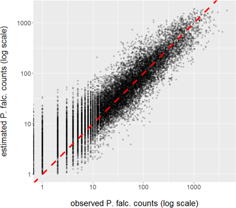
Observed cases of P. falciparum malaria, by district and week, vs. counts estimated by the best model from the GA. The red, dashed line indicates the points at which observed is exactly the estimated value.

When evaluated on the original scale of the data (cases per district per week), the model had mean absolute error (MAE) 43 cases, root mean square error (RMSE) 114 cases, R-squared of observed versus predicted 0.825, and Spearman correlation of observed versus predicted 0.917. This model’s performance varies by cluster (Table 2), with MAE ranging from 12–77, RMSE ranging from 21–168, R2 ranging from 0.70–0.90, and Spearman correlation ranging from 0.83–0.93.

Table 2:

Error statistics for the best model selected by genetic algorithm, trained on all available data, evaluated per cluster.

cluster	MAE	RMSE	R2	Spearman
A	31	103	0.901	0.902
B	44	114	0.825	0.934
C	74	154	0.786	0.865
D	77	168	0.704	0.902
E	12	21	0.787	0.825
F	30	55	0.883	0.901

The six clusters of the model, displayed in Figure 3, tended to cohere spatially. It should be noted that the spatial configuration of districts was not explicitly considered by the GA, and clustering is determined solely by observed responses to covariates; this result implies that nearby districts do tend to respond similarly to environmental drivers of human malaria cases. However, some areas, particularly the lowland districts on the shores of Lake Tana, contained adjacent districts belonging to different clusters.

Figure 3:

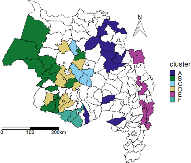
The clusters assigned by the best model of P. falciparum malaria in 750 generations of the genetic algorithm described above. Districts in white did not report data and were not modeled. Districts in the same cluster had the same estimated responses to environmental covariates, even if the districts did not share the same long-term trends.

After removing the long-term trend from every district with the simplified model using only the first three, long-term terms of the basic model (i.e. γ_cib = 0), differences among the clusters were clearer (Figure 4). There were a variety of behaviors, coherent within each cluster but differing among clusters. For example, clusters C and D both exhibited distinctive early season malaria peaks in 2013 and 2016. In addition, a large malaria outbreak occurred in cluster C in 2014, but was not apparent in cluster D, whereas there was an early season malaria outbreak in cluster D in 2015 that did not occur in cluster C.

Figure 4:

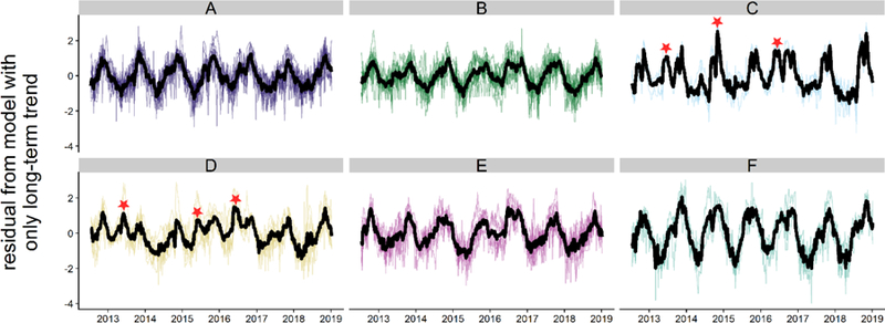
Residuals from the simplified model in which P. falciparum malaria cases depend only on the long-term trend in every district. The mean residual for every cluster is in black, and the differences in these lines are the differences to be explained by environmental covariates in the basic model. Notable deviations from the regular seasonal pattern are marked in the graph and discussed in the text.

The GA was designed to explain these deviations in terms of environmental covariates, and estimated dependence on past environmental conditions did vary among clusters (Figure 5). Temporal variation in malaria depended strongly on precipitation (PMMC), with risk relating positively in all clusters to precipitation at lags of 70 to 120 days. The most unusual cluster C showed particularly strong responses to more recent ( ≈ 45 day lag) PMMC. Cluster D, which also exhibited several outbreaks deviating from the seasonal pattern, correlated positively with PMMC over a wider range of lags from zero to 150 days. Malaria in these two clusters also correlated positively with temperature (LSTM) at lags of 10 to 100 days and negatively with the water index (NDWI6) at lags less than 30 days.

Figure 5:

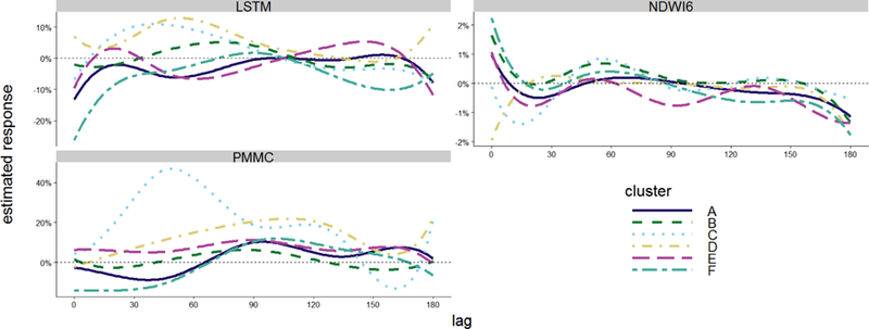
Estimated response of P. falciparum cases to LSTM, NDWI6, and PMMC at different lags. The estimated value gives the expected percentage change in cases for districts in that cluster if the covariate were increased by one standard deviation at some lag before the week in question began. Hence, falling on the dashed line at 0% indicates that changes in the environment at that lag are estimated to be irrelevant to risk today.

Cluster B also exhibited mostly positive lagged relationships with precipitation and temperature, although the response of malaria to these climatic factors was weaker than clusters C and D, and there was also a positive correlation with the water index at the shortest lags. Thus, all the clusters located in the wetter, northwestern part of the Amhara region consistently exhibited positive lagged relationships with temperature and precipitation. In contrast, lagged relationships with temperature and precipitation were more complex with clusters A, E, and F, which were located farther to the east and south. In these generally drier parts of the region, the relationships of malaria with temperature and precipitation tended to vary from negative to positive different lags. These three clusters also exhibited positive associations with the water index at the shortest lags combined with a positive and negative associations at longer lags.

4. Discussion

We used an evolutionary algorithm to simultaneously solve the problems of variable selection and determine the optimal spatial stratification of an environmentally driven time-series model of malaria in the Amhara region of Ethiopia. The algorithm grouped districts into six clusters based on responses to environmental inputs. The districts within each of these six clusters shared a set of distributed lag functions that modeled the delayed effects of temperature and moisture conditions over the past 180 days. The best six-cluster model was superior to alternative models in which the districts were aggregated into smaller or larger numbers of clusters. By applying the genetic algorithm, we were able to identify an optimal set of clusters based on the modeled relationships between malaria and its environmental drivers rather than having to arbitrarily select a stratification a priori based on epidemiological or environmental proxies.

Although the algorithm combined districts without regard to geographic location, the resulting clusters exhibited some degree of spatial patterning. In particular, the clusters located in the northwestern part of the Amhara region exhibited distinctive environmental relationships compared with clusters in the eastern and southern parts of the region. This pattern is consistent with the expectation that nearby locations share similar ecological and social characteristics, so that malaria transmission is likely to respond similarly to changes in environmental conditions. The western parts of Amhara generally receive more precipitation and have a longer rainy season than the eastern parts (Midekisa et al. 2015), and these climatological differences may partially account for the differences in environmental sensitivities across the clusters identified by our model. Other factor such as hydrology, land use, human population density, and levels of seasonal migration likely also contribute to the differences in environmental responses among the clusters. We do also find that some clusters, especially those in the districts surrounding Lake Tana, do not necessarily cohere spatially; partitioning the districts by responses to environmental covariates was not as simple as noting proximity. Further analysis of these clusters can provide additional insights into the geographic factors that explain differences in the environmental epidemiology of malaria throughout the region.

The model’s predictions were generally accurate but varied across the six clusters. Model fit was best in cluster A, which included many of the driest districts in the eastern part of the region, and cluster F, which was a small cluster of three districts on the edge of the Blue Nile escarpment. In contrast, clusters C and D had the least accurate predictions. These clusters are located mainly in lower-elevation areas surrounding Lake Tana where malaria incidence has historically been high and large outbreaks have occurred. The high accuracy in clusters A and F can be attributed to the strong seasonal signal with relatively minor deviations in any given year as shown in Figure 4. In contrast, the more irregular patterns of outbreaks in clusters C and D are more challenging to predict, resulting in a weaker fit to the environmental model.

The genetic algorithm selected one temperature variable (LSTM), one precipitation variable (PMMC), and one spectral water index (NDWI6) as covariates in the best model. Temperature is well-established as an important predictor of mosquito population dynamics and parasite transmission rates, and precipitation is a critical source of water for breeding habitats (Stresman 2010). Remotely-sensed vegetation and water indices have also been shown to serve as indicators of environmental factors that influence malaria transmission (Cohen et al. 2013; Midekisa et al. 2012). The specific malaria responses to these environmental factors varied considerably across cluster, encompassing positive as well as negative responses. This diversity of responses is expected given the non-linear responses of mosquito and parasite life-history traits to temperature (Mordecai et al. 2013), and the potential for precipitation to have either positive or negative effects on mosquito populations (Paaikmans et al. 2007). Abeku et al. found that malaria epidemics occurring at different times at different locations were triggered by different sets of environmental anomalies, and they emphasized that these non-uniform effects need to be accounted for in epidemic early-warning models (Abeku et al. 2003). Imai et al. found that relationships between environmental covariates and malaria incidence in New Guinea even changed direction across regions (Imai et al. 2016).

The genetic algorithm had the options of selecting spatially homogeneous (one cluster) or heterogeneous (forty-seven cluster) models, where all districts responded either identically or independently to environmental variability, but indicated instead that there were six, rather than one or forty-seven, sets of distinctive malaria-environmental relationships in the region. Despite the sensible belief that the truth is between complete homogeneity and heterogeneity, we find that most choices in the literature fall at those extremes and are made a priori. For example, in a model of malaria in Ethiopia by Abeku et al., relationships with some covariates varied for each of the 35 areas studied, while others were common to all (Abeku et al. 2004). In a model of West Nile virus in the United States, relationships were shared by all counties in the contiguous US (Manore et al. 2014). The acknowledgment that a choice has even been made is relatively rare; Jaya et al. present one of the few examples comparing spatially homogeneous to heterogeneous models, noting that spatially-varying models outperformed those with fixed coefficients (Jaya et al. 2016).

The primary strength of the evolutionary approach for model selection and spatial stratification is its flexibility and ease of implementation. All that is typically necessary is a method of ranking models and small set of rules for mutation and reproduction. In this application, we selected a negative binomial model that predicted malaria as distributed lag functions of environmental variables combined with a long-term trend component as the most appropriate given the characteristics of our data. However, the approach could potentially be extended to different types of generalized linear models (e.g. Gaussian, Poisson, or binomial) and to different specifications of the time series model.

However, this flexibility also reveals the algorithm’s primary weakness. No domain-specific knowledge is necessary for this generalized algorithm, so the algorithm is considered “blind” or “weak” and will likely be outperformed by algorithms specifically designed for the problem (Whitley 2001). For example, these data concern an infectious disease, which probably displays spatial autocorrelation in outcome. Dengue for example has been observed to travel in waves, and these are unlikely to be explained solely by referencing environmental covariates (Churakov et al. 2019). Conditional-autoregressive models and models with spatially-varying coefficients could also be considered (Alegana et al. 2013; Arab, Jackson, and Kongoli 2014). A more comprehensive spatial sample would have been necessary to permit such an analyses in the present application. Additionally, the version of the genetic algorithm that we used is relatively simple among its peers. Thus, it could be modified to accelerate convergence or more thoroughly or efficiently explore the space of models (Liao 2005; Pattarin, Paterlini, and Minerva 2004; Rani and Sikka 2012).

4.1. Conclusion

A genetic algorithm proved to be effective for selecting cluster memberships and parameters to develop a parsimonious model of environmentally-driven malaria outbreaks across a heterogeneous region in the highlands of Ethiopia. This method of clustering and prediction is currently being implemented in the Amhara region as part of a regional system integrating disease surveillance with environmental monitoring for malaria early warning (Merkord et al. 2017). In addition to yielding an improved forecasting model, the accompanying stratification of districts with similar environmental sensitivities can be helpful in planning regional malaria control and elimination efforts. Although the model uses environmental data up to the week in question, the strongest effects of temperature and precipitation on risk are for most clusters far enough in the past that increased risk of outbreaks can be detected in advance. Application of insecticides, distribution of insecticide-treated nets, and preventative treatment may be more accurately scheduled, increasing the cost-effectiveness of interventions (White et al. 2011). For example, malaria had strong lagged associations with environmental covariates in clusters C and D, and local outbreaks deviating from the expected season patterns were most pronounced in these areas. Thus, abnormally high temperature and precipitation in these regions would result in a forecast of higher-than-normal malaria cases, triggering the public health system to increase the availability of malaria drugs and other health care services an implement with vector-control measures such as indoor residual spraying, distribution of long-lasting insecticide-treated bed nets (LLINs), and source control to eliminate breeding habitats.

Future work will include examining a larger set of predictors, especially the socioeconomic, human movement, clinical, and land-use variables that have elsewhere shown promise as predictors (Baeza et al. 2017; Thakur and Dharavath 2019; Valle and Lima 2014; Wesolowski et al. 2012). Further extensions of this technique could explore various modifications, including methods to speed up convergence when modeling larger data sets. This spatially-stratified modeling approach could also be extended to other diseases and different types of ecological forecasting problems where spatial non-stationarity is likely to be an important factor, including models of wildfire risk (Chuvieco et al. 2010) and agricultural productivity (Becker-Reshef et al. 2010) as a function of climate data. More generally, we suggest that addressing spatial non-stationarity in environmental relationships is an important consideration when modeling and forecasting environmentally sensitive phenomena. By using a model-based clustering strategy such as the one presented here, it is possible to improve the fit of statistical time series models while also gaining insights into the contextual factors that condition environmental responses.

• Time series of malaria in the Amhara region of Ethiopia can be modeled with remotely-sensed environmental covariates and a long-term trend.

• Responses to climate variations are not uniform over the whole study area and the space needs to be partitioned into separate models.

• A simple genetic algorithm successfully partitioned districts into clusters with homogeneous responses to lagged environmental data.

• The patterns of malaria outbreaks and their sensitivities to environmental variables varied geographically along a precipitation gradient.

Appendix

Appendix Figure 1:

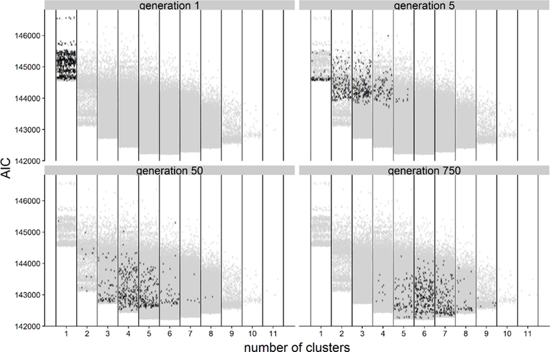
Model performance as a function of generation and number of clusters in the model. Models in the indicated generation are displayed in black. Models from all other generations are displayed in grey for comparison. Points are jittered along the x-axis to assist in visualizing density.

Appendix Figure 2:

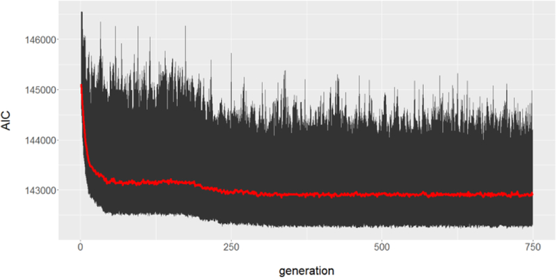
Model performance as a function of generation. The mean of the AIC of all models in a generation is in red, while max/min for that generation are displayed in black.

References

- Abeku TA, DeVlas SJ, Borsboom GJ, Tadege A, Gebreyesus Y, Gebreyohannes H, Alamirew D, Seifu A, Nagelkerke NJ, and Habbema JD 2004. ‘Effects of meteorological factors on epidemic malaria in Ethiopia: a statistical modelling approach based on theoretical reasoning.’, Parasitology, 128: 585–93. [DOI] [PubMed] [Google Scholar]
- Abeku TA, vanOortmarssen GJ, Borsboom G, deVlas SJ, and Habbema JDF 2003. ‘Spatial and temporal variations of malaria epidemic risk in Ethiopia: factors involved and implications’, Acta Tropica, 87: 331–40. [DOI] [PubMed] [Google Scholar]
- Alegana VA, Atkinson PM, Wright JA, Kamwi R, Uusiku P, Katokele S, Snow RW, and Noor AM 2013. ‘Estimation of malaria incidence in northern Namibia in 2009 using Bayesian conditional-autoregressive spatial–temporal models’, Spatial and Spatio-temporal Epidemiology, 7: 24–36. [DOI] [PMC free article] [PubMed] [Google Scholar]
- Almon Shirley. 1965. ‘The distributed lag between capital appropriations and expenditures’, Econometrica: Journal of the Econometric Society: 178–96.
- Alonso P, and Noor AM 2017. ‘The global fight against malaria is at crossroads’, The Lancet, 390: 2532–34. [DOI] [PubMed] [Google Scholar]
- Arab A, Jackson MC, and Kongoli C 2014. ‘Modelling the effects of weather and climate on malaria distributions in West Africa’, Malaria Journal, 13. [DOI] [PMC free article] [PubMed] [Google Scholar]
- Baeza Andres, Santos-Vega Mauricio, Dobson Andrew P, and Pascual Mercedes 2017. ‘The rise and fall of malaria under land-use change in frontier regions’, Nature ecology & evolution, 1: 0108. [DOI] [PubMed] [Google Scholar]
- Becker-Reshef I, Vermote E, Lindeman M, and Justice C 2010. ‘A generalized regression-based model for forecasting winter wheat yields in Kansas and Ukraine using MODIS data’, Remote Sensing of Environment, 114: 1312–23. [Google Scholar]
- Brady OJ, Gething PW, Bhatt S, Messina JP, Brownstein JS, Hoen AG, Moyes CL, Farlow AW, Scott TW, and Hay SI 2012. ‘Refining the Global Spatial Limits of Dengue Virus Transmission by Evidence-Based Consensus’, PLOS Neg Trop Dis [DOI] [PMC free article] [PubMed]
- Burnham KENNETHP, and Anderson DAVfD R 2002. ‘A practical information-theoretic approach’, Model selection and multimodel inference, 2nd ed. Springer, New York. [Google Scholar]
- Ceccato P, Ghebremeskel T, Jaiteh M, Graves PM, Levy M, Ghebreselassie S, Ogbamariam A, Barnston AG, Bell M, delCorral J, Connor SJ, Fesseha I, Brantly EP, and Thomson MC 2007. ‘Malaria stratification, climate, and epidemic early warning in Eritrea’, Am J Trop Med Hyg, 77: 61–68. [PubMed] [Google Scholar]
- Ceccato P, Vancutsem C, Klaver R, Rowland J, and Connor SJ 2012. ‘A Vectorial Capacity Product to Monitor Changing Malaria Transmission Potential in Epidemic Regions of Africa’, J Trop Med [DOI] [PMC free article] [PubMed]
- Chen D, Huang J, and Jackson TJ 2005. ‘Vegetation water content estimation for corn and soybeans using spectral indices derived from MODIS near- and short-wave infrared bands’, Rem Sens Environ, 98: 225–36. [Google Scholar]
- Churakov Mikhail, Villabona-Arenas Christian J, Kraemer Moritz UG, Salje Henrik, and Cauchemez Simon. 2019. ‘Spatio-temporal dynamics of dengue in Brazil: seasonal travelling waves and determinants of regional synchrony’, PLoS neglected tropical diseases, 13: e0007012. [DOI] [PMC free article] [PubMed] [Google Scholar]
- Chuvieco E, Aguado I, Yebra M, Nieto H, Salas J, Martin MP, Vilar L, Martinez J, Martin S, Ibarra P, delaRiva J, Baeza J, Rodriguez F, Molina JR, and Herrera MA Zamora R 2010. ‘Developmnt of a gramework for fire risk assessment using remote sensing and geographic information system tecnologies’, Ecological Modelling, 221: 46–58. [Google Scholar]
- Cohen JM, Dlamini S, Novotny JM, Kandula D, Kunene S, and Tatem AJ 2013. ‘Rapid case-based mapping of seasonal malaria transmission risk for strategic elimination planning in Swaziland’, Malaria Journal, 12. [DOI] [PMC free article] [PubMed] [Google Scholar]
- De Boor Carl, Carl De Boor, Mathématicien Etats-Unis, De Boor Carl, and De Boor Carl 1978. A practical guide to splines (springer-verlag New York; ). [Google Scholar]
- Falkenauer E 1998. Genetic Algorithms and Grouping Problems (John Wiley & Sons, Inc.: New York, NY: ). [Google Scholar]
- Gao BC. 1996. ‘NDWI—a normalized difference water index for remote sensing of vegetation liquid water from space’, Rem Sens Environ, 58: 257–66. [Google Scholar]
- Geerken R, Zaitchik B, and Evans JP 2005. ‘Classifying rangeland vegetation type and coverage from NDVI time series using Fourier Filtered Cycle Similarity’, International Journal of Remote Sensing, 26: 5535–54. [Google Scholar]
- Goldberg David E, and Deb Kalyanmoy 1991. ‘A comparative analysis of selection schemes used in genetic algorithms.’ in, Foundations of genetic algorithms (Elsevier; ). [Google Scholar]
- Huete AR 1988. ‘A soil-adjusted vegetation index (SAVI)’, Remote Sensing of Environment: 295–309.
- Huffman GJ, Bolvin DT, Nelkin EJ, Wolff DB, Adler RF, and Gu G 2007. ‘The TRMM multisatellite precipitation analysis (TMPA): quasi-global, multiyear, combined-sensor precipitation estimates at fine scales’, J Hydrometeorol, 8: 38–55. [Google Scholar]
- Imai C, Cheong HK, Kim H, Honda Y, Eum JH, im CT, Kim JS, Kim Y, Behera SK, Hassan MN, Nealon J, Cuhng H, and Hashizume M 2016. ‘Associations between malaria and local and global climate variability in five regions in Papua New Guinea’, Trop Med and Health, 44. [DOI] [PMC free article] [PubMed] [Google Scholar]
- Jaya I, Abdullah A, Hermawan E, and Ruchjana B 2016. ‘Bayesian Spatial Modeling and Mapping of Dengue Fever: A Case Study of Dengue Feverin the City of Bandung, Indonesia’, Int J Applied Math and Stat, 54. [Google Scholar]
- Jiang Z, Huete AR, Didan K, and Miura T 2008. ‘Development of a two-band enhanced vegetation index without a blue band’, Rem Sens Environ, 112: 3833–45. [Google Scholar]
- Kulldorff Martin, Mostashari Farzad, Duczmal Luiz, Katherine Yih W, Kleinman Ken, and Platt Richard. 2007. ‘Multivariate scan statistics for disease surveillance’, Statistics in medicine, 26: 1824–33. [DOI] [PubMed] [Google Scholar]
- Li Yifeng, and Ngom Alioune. 2013. ‘The non-negative matrix factorization toolbox for biological data mining’, Source code for biology and medicine, 8: 10. [DOI] [PMC free article] [PubMed] [Google Scholar]
- Liao T Warren. 2005. ‘Clustering of time series data—a survey’, Pattern recognition, 38: 1857–74. [Google Scholar]
- Liu Y, Hu J, Snell-Feikema I, VanBemmel MS, Lamsal A, and Wimberly MC 2015. ‘Software to facilitate remote sensing data access for disease early warning systems’, Environmental Modelling & Software, 74: 247–57. [DOI] [PMC free article] [PubMed] [Google Scholar]
- Lowe R, Chirombo J, and Tompkins AM 2013. ‘Relative importance of climatic, geographic and socio-economic determinants of malaria in Malawi’, Malaria Journal, 12. [DOI] [PMC free article] [PubMed] [Google Scholar]
- Manore CA, Davis JK, Christofferson RC, Wesson DM, Hyman JM, and Mores CN 2014. ‘Towards an early warning system for forecasting human West Nile virus incidence’, PLoS Currents, 6. [DOI] [PMC free article] [PubMed] [Google Scholar]
- Maulik U, and Bandyopadhyay S 2000. ‘Genetic algorithm-based clustering technique’, Pattern Recognition, 33: 1455–65. [Google Scholar]
- Merkord CL, Liu Y, Mihretie A, Gebrehiwot T, Awoke W, Bayabil E, Henebry GM, Kassa GT, Lake M, and Wimberly MC 2017. ‘Integrating malaria surveillance with climate data for outbreak detection and forecasting: the EPIDEMIA system’, Malaria Journal, 16. [DOI] [PMC free article] [PubMed] [Google Scholar]
- Midekisa A, Beyene B, Mihretie A, Bayabil E, and Wimberly MC 2015. ‘Seasonal associations of climatic drivers and malaria in the highlands of Ethiopia’, Parasites & Vectors, 8. [DOI] [PMC free article] [PubMed] [Google Scholar]
- Midekisa A, Senay G, Henebry GM, Semuniguse P, and Wimberly MC 2012. ‘Remote sensing-based time series models for malaria early warning in the highlands of Ethiopia’, Malaria Journal, 11. [DOI] [PMC free article] [PubMed] [Google Scholar]
- Mordecai EA, Paaijmans KP, Johnson LR, Balzer C, Ben-Horin T, Moor E, McNally A, Pawar S, Ryan SJ, Smith TC, and Lafferty KD 2013. ‘Optimal temperature for malaria transmission is dramatically lower than previously predicted’, Ecology Letters, 16: 22–30. [DOI] [PubMed] [Google Scholar]
- Olson Sh, Gangnon R, Elguero E, Durieux L, Guegan JF, Foley JA, and Patz JA 2009. ‘Links between Climate, Malaria, and Wetlands in the Amazon Basin’, Emerg Infect Dis, 15: 659–62. [DOI] [PMC free article] [PubMed] [Google Scholar]
- Paaikmans KP, Wandago MO, Githeko AK, and Takken W 2007. ‘Unexpected High Losses of Anopheles gambiae Larvae Due to Rainfall’, PLoS ONE [DOI] [PMC free article] [PubMed]
- Pattarin Francesco, Paterlini Sandra, and Minerva Tommaso. 2004. ‘Clustering financial time series: an application to mutual funds style analysis’, Computational Statistics & Data Analysis, 47: 353–72. [Google Scholar]
- Rani Sangeeta, and Sikka Geeta. 2012. ‘Recent techniques of clustering of time series data: a survey’, International Journal of Computer Applications, 52. [Google Scholar]
- RCoreTeam. 2018. ‘R: A language and environment for statistical computing’, R Foundation for Statistical Computing, Accessed 01 Jan. https://www.r-project.org/. [Google Scholar]
- Schwaller MR, and Morris KR 2011. ‘A ground validation network for the Global Precipitation Measurement Mission’, J Atmo and Ocean Tech, 28. [Google Scholar]
- Stresman GH. 2010. ‘Beyond temperature and precipitation: ecological risk factors that modify malaria transmission’, Acta Tropica, 116: 167–72. [DOI] [PubMed] [Google Scholar]
- Teklehaimanot HD, Lipsitch M, Teklehaimanot A, and Schwartz J 2004. ‘Weather-based prediction of Plasmodium falciparum malaria in epidemic-prone regions of Ethiopia’, Malaria Journal, 3. [DOI] [PMC free article] [PubMed] [Google Scholar]
- Thakur Santosh, and Dharavath Ramesh. 2019. ‘Artificial neural network based prediction of malaria abundances using big data: A knowledge capturing approach’, Clinical Epidemiology and Global Health, 7: 121–26. [Google Scholar]
- Thomson MC, and Connor SJ 2001. ‘The development of Malaria Early Warning Systems for Africa’, Trends in Parasitology, 17: 438–45. [DOI] [PubMed] [Google Scholar]
- Tucker CJ. 1979. ‘Red and photographic infrared linear combinations for monitoring vegetation’, Rem Sens Environ, 8: 127–50. [Google Scholar]
- Valle Denis, and Tucker Lima Joanna M 2014. ‘Large-scale drivers of malaria and priority areas for prevention and control in the Brazilian Amazon region using a novel multi-pathogen geospatial model’, Malaria Journal, 13: 443. [DOI] [PMC free article] [PubMed] [Google Scholar]
- Venables WN, Ripley BD, and Springer Isbn. 2002. ‘Statistics Complements to Modern Applied Statistics with S Fourth edition by’
- Vlachos Michail, Lin Jessica, Keogh Eamonn, and Gunopulos Dimitrios. 2003. “A wavelet-based anytime algorithm for k-means clustering of time series.” In In proc. workshop on clustering high dimensionality data and its applications Citeseer. [Google Scholar]
- Wan Z 2008. ‘New refinements and validation of the MODIS land-surface temperature/emissivity products’, Rem Sens Eviron, 112: 59–74. [Google Scholar]
- Wesolowski Amy, Eagle Nathan, Tatem Andrew J, Smith David L, Noor Abdisalan M, Snow Robert W, and Buckee Caroline O 2012. ‘Quantifying the impact of human mobility on malaria’, Science, 338: 267–70. [DOI] [PMC free article] [PubMed] [Google Scholar]
- White Michael T, Conteh Lesong, Cibulskis Richard, and Ghani Azra C 2011. ‘Costs and cost-effectiveness of malaria control interventions-a systematic review’, Malaria journal, 10: 337. [DOI] [PMC free article] [PubMed] [Google Scholar]
- Whitley D 2001. ‘An overview of evolutionary algorithms: practical issues and common pitfalls’, Informatino and Software Technology, 43: 817–31. [Google Scholar]
- Wilder-Smith A, Gubler DJ, Weaver SC, Monath TP, Heymann DL, and Scott TW 2017. ‘Epidemic arboviral diseases: priorities for research and public health’, The Lancet, 17: 101–06. [DOI] [PubMed] [Google Scholar]
- Wimberly MC, Midekisa A, Semuniguse P, Teka H, Henebry GM, Chuang TW, and Senay GB 2012. ‘Spatial synchrony of malaria outbreaks in a highland region of Ethiopia’, Trop Med & Int Health, 17: 1192–201. [DOI] [PMC free article] [PubMed] [Google Scholar]
- Zinszer K, Kigozi R, Charland K, Dorsey G, Brewer TF, Brownstein JS, Kamya MR, and Buckeridge DL 2015. ‘Forecasting malaria in a highly endemic country using environmental and clinical predictors’, Malaria Journal, 14. [DOI] [PMC free article] [PubMed] [Google Scholar]