Abstract
Objective: In this research, a marker-less ‘smart hallway’ is proposed where stride parameters are computed as a person walks through an institutional hallway. Stride analysis is a viable tool for identifying mobility changes, classifying abnormal gait, estimating fall risk, monitoring progression of rehabilitation programs, and indicating progression of nervous system related disorders. Methods: Smart hallway was build using multiple Intel RealSense D415 depth cameras. A novel algorithm was developed to track a human foot using combined point cloud data obtained from the smart hallway. A method was implemented to separate the left and right leg point cloud data, then find the average foot dimensions. Foot tracking was achieved by fitting a box with average foot dimensions to the foot, with the box’s base on the foot’s bottom plane. A smart hallway with this novel foot tracking algorithm was tested with 22 able-bodied volunteers by comparing marker-less system stride parameters with Vicon motion analysis output. Results: With smart hallway frame rate at approximately 60fps, temporal stride parameter absolute mean differences were less than 30ms. Random noise around the foot’s point cloud was observed, especially during foot strike phases. This caused errors in medial-lateral axis dependent parameters such as step width and foot angle. Anterior-posterior dependent (stride length, step length) absolute mean differences were less than 25mm. Conclusion: This novel marker-less smart hallway approach delivered promising results for stride analysis with small errors for temporal stride parameters, anterior-posterior stride parameters, and reasonable errors for medial-lateral spatial parameters.
Keywords: Foot tracking, Intel RealSense D415, marker-less, smart hallway, stride analysis
I. Introduction
Human stride analysis in clinical settings is often performed with optical marker tracking systems such as Vicon, Optitrack, and Qualisys, requiring expensive setup, specialized human resources, and dedicated laboratory space. Passive or active markers, such as light-emitting diodes, are placed on the body to track limbs for human gait acquisition and characterization [1]. Inertial Measurement Units (IMU) can also be attached to body parts to record inertial motion based [2] kinematic gait data. Affixing external sensors on the human body may cause discomfort to patients and substantially change their natural gait [3]. These systems also require technical expertise for attaching markers and conducting experiments.
Low-cost Kinect depth sensors for gaming showed potential for human gait-related health care applications; such as, fall risk [4]–[6], Parkinson’s disease movement assessment [7], fall detection of people with multiple sclerosis [8], autism disorder identification [9], abnormal gait classification [10], [11], virtual gait training [12], diagnosis, monitoring, and rehabilitation [13]. Depth sensors capture both depth and color images. Depth data contains distances, at each pixel, between the depth sensor and objects in the capturing scene. With this depth information, the real 3D coordinates at each pixel are recorded, with the depth sensor as the origin (i.e., “point cloud”). Most research on depth sensors for human movement analysis involved Microsoft Kinect. Kinect V2 systems can identify and track the majority of human joints by defining joint locations that constitute a human skeleton-model or building a human model from the scene’s point cloud. However, gaps and limitations exist with frame rate [14] and lower body tracking, especially at the ankle and foot [14], [15]. Multiple Kinect V2 sensors can capture longer volumes, with promising results, but ankle tracking farther from the sensor was more inconsistent [16]. Kinect’s machine learning-based skeleton tracking was not reliable, with tracking points sometimes moving outside the body and tracking varying with viewing angle [17]. Given these limitations, approaches that use the whole point cloud could provide better foot tracking results.
Patients, staff, and visitors typically move through similar hallways in hospitals, rehabilitation centers, or long-term care facilities [18]. This space could be utilized in an intelligent way by building a system to perform marker-less stride analysis as patients or residents walk through the hallway. Measuring patients every time they walk through the hallway, without intervention, could help identify changes in their movement status. To capture multiple strides and avoid occlusions while a person is walking, multiple depth sensors would be required. Unlike time-of-flight based Kinect V2 sensor, Stereoscopic infra-red based Intel RealSense D415 depth sensors were shown to be suitable for this application since they did not experience interference when multiple sensors were used simultaneously [19]. Furthermore, these sensors capture data at 60fps, which can provide sufficient data for analyzing temporal related stride parameters.
This research explored depth sensing technology for stride parameter analysis within an institutional hallway environment. The main contributions were developing, prototyping, and validating a novel point-cloud-based marker-less system with an innovative foot tracking algorithm and assessed system performance by comparing stride parameter output with industry standard marker-based motion analysis. Successful implementation of this smart hallway concept would introduce unobtrusive movement status assessment that can guide clinical decision-making, without introducing unsustainable human resource requirements. This would also become the basis for future data analytics applications for predicting changes in dementia, fall risk, or other aging-related conditions.
II. System Setup and Synchronization
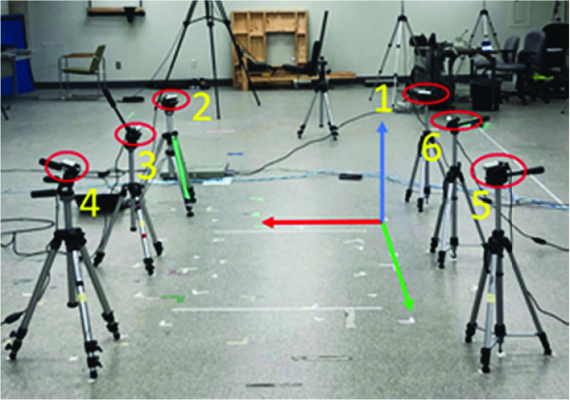
In our previous work [20], a physical setup with six Intel RealSense D415 sensors was configured in the lab to replicate a hallway scenario (Fig. 1). These sensors were placed at 0.8m height from the floor, with 1.4m between adjacent sensors in y-axis (i.e., (1,6), (2,3), (3,4), (5,6)), and 1.8m in x-axis direction (i.e., (1,2), (3,6) and (4,5)). Techniques from this research were used for temporal synchronization (client-server approach) and spatial synchronization (stereo chess board method).
FIGURE 1.
Physical setup of the marker-less system using hallway dimensions (Red: x-axis, Green: y-axis, and Blue: z-axis).
The new smart hallway system captures  pixel depth images and color images at approximately 60fps (frame rate varies slightly because of buffer time for transmitting data through Ethernet after capturing each frame), with a timestamp for each frame, from all the six sensors. To increase accuracy and reduce computation time, a non-zero median filter for every
  pixels was applied to remove “spikes” in the depth data and down-sample to half resolution (
 ) [21].
A. Sensor Parameters
Intrinsic parameters such as focal length ( ) and principal point (
 for Intel RealSense D415 depth and color cameras were obtained from the manufacturer. Two coordinate systems (depth, color) and extrinsic parameters (rotation and translation, to transform data between depth and color coordinate systems) were also obtained. This marker-less six depth sensors setup was spatially synchronized in the color coordinate system, such that the combined output point cloud was in the first sensor’s color coordinate system.
B. Room Coordinate System
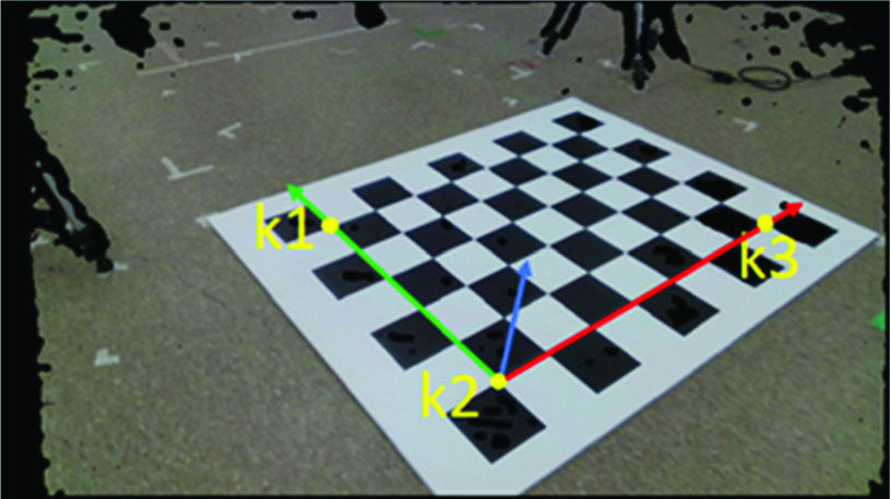
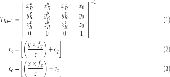
A reference coordinate system on the floor plane (Fig. 1) was designed using a chessboard (Fig. 2), with x-axis in the medial-lateral (ML) walking direction, y-axis parallel to the walking pathway (anterior-posterior; AP), and z-axis outwards to the floor (Vertical; V). This reference coordinate system was labelled as the Room Coordinate System (RCS). Methods from our previous study [20] were used to transform point cloud data from all the sensors into the first sensor’s color coordinate system, then transformed into the RCS by determining a transformation matrix  (1).
(1).
FIGURE 2.
Key points on the chessboard for room coordinate system (Red: x-axis, Green: y-axis, and Blue: z-axis).
A  chessboard was placed on the floor with the horizontal edge parallel to the RCS x-axis and vertical edge parallel to the y-axis. The board’s depth and color images were captured with the first sensor at
  resolution. The depth image was down-sampled to half resolution using median filter. 3D points were calculated from the depth image using depth intrinsic parameters and then the points were transformed into the color coordinate system using extrinsic parameters.
A new color image was constructed using 3D points and corresponding projection pixels onto the captured color image. For a 3D point ( ) in the color coordinate system corresponding to row
  and column
  in the depth image, the projected pixel location (
 ) in the captured color image was found using equations (2) and (3) (color camera’s intrinsic parameters). The red, green, and blue channel values at row
  and column
  in the constructed color image (Fig. 2) were the values at row
  and column
  in the captured color image and the values of pixels corresponding to invalid 3D data (0,0,0) were set to zeroes.
Three key points  and
and  were identified in 100 frames. For each key point, 100 instants of its 3D location were obtained in the color coordinate system. Each dimension value (
 ,
,  ,
,  ) of these 100 3D points was sorted separately and the middle 50 values were averaged.
The RCS origin was at point  , the unit vectors were
  from
from  to
to  ,
,  from
from  to
to  , and
, and  the cross product of
  and
and  with respect to the first sensor color coordinate system, whose origin was at the point (0, 0, 0) and corresponding unit vectors were
  ,
,  , and
, and  , respectively. The transformation matrix from the first sensor to the RCS was obtained using (1).
III. Point Cloud
A point cloud was generated from the six depth sensors. The process involved generating a background depth image from a static scene, subtracting the background information from the depth images, constructing walking human point cloud data for each sensor from the background subtracted depth images, and merging and transforming point clouds from the six sensors to RCS. The combined point cloud was filtered and smoothed to reduce noise.
A. Background Frame
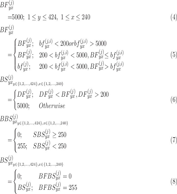
From each sensor, 1000 depth frames of background data (without any objects) were captured. The pixel value at row  , column
  of these background frames was represented as
  for the
  frame of the
  sensor. This system was designed to work in the range of 200mm to 5000mm. All background frame pixels for the
  sensor
  were initialized with 5000 (4), then the pixel value at row
  , column
  was updated with the minimum of
  and
and  , iterating through 1000 frames (
 to 1000) using eq. (5).
B. Background Subtraction
A background subtracted depth image for the  sensor
  was obtained by pixel-wise comparison with the corresponding sensor’s background frame
  [22]. For a depth frame from the
  sensor
  , pixel values less than the background frame’s pixel value, and greater than the minimum value (200 mm), were considered the same value in the
  frame. Other pixel values were assigned the maximum value (5000 mm), as presented in eq. (6), for a pixel in
  row and
  column. For further processing,
  was linearly scaled down to [0, 255] from [0, 5000].
 |
From the scaled-down image  , a Binary Background Subtracted image
  was constructed based on eq. (7).
A connected component filter [23] with 1000 pixels connected area cut-off was applied to the  image and output was a Binary Filtered Background Subtracted image
  . The
. The  image was modified based on the
  , pixel locations with zero value in
  were assigned to zero in
  frame (8). Sample
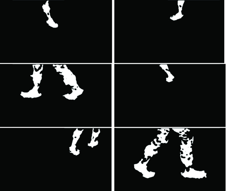
  frames from all sensors are shown in Fig. 3. White pixels in the
  frames were foreground and black pixels were background. Depth data was not captured in the small gaps among foreground pixels.
FIGURE 3.
Background subtracted binary images from six sensors.
C. Point Cloud Construction
3D point cloud points were constructed from each sensor’s background-subtracted depth images and then transformed into the first sensor’s coordinate system [20]. This “combined point cloud” points were transformed into RCS by multiplying with transformation matrix  , obtained from (1).
 |
D. Point Cloud Filtering
The combined point cloud was filtered using a statistical outlier filter [24], smoothed with a moving least-squares technique [25], and then down-sampled with a voxel grid filter [26]. OpenCV libraries [27] were used for 2D image processing and PCL [28] for 3D point cloud processing.
For every 3D point in a point cloud, 100 neighbor points were analyzed to find outliers. Mean and standard deviation of distances of the closest 100 points from each point of interest were found. Points farther than one standard deviation from the point of interest were considered outliers and removed.
Point cloud points were smoothed by fitting a second-order polynomial equation to points within 30 mm of each point of interest in the point cloud. The point cloud was divided into 5mm  mm
mm  mm voxels (3D boxes) and then down-sampled by replacing points in a voxel with the centroid of these points. This method of down-sampling retained the point cloud surface and reduced computation time for point cloud processing.
IV. Leg Segmentation
Since this application tracks a walking person’s foot, point cloud points less than 70 cm from the floor were selected, since the foot and shank are always present in this region. The free parameters presented in the following sections were tuned to fit the foot tracking algorithm to an adult’s (between 5 feet and 6 feet height) leg dimension and also based on the point cloud density obtained from six Intel RealSense D415 sensors. These parameters could be fine-tuned based on the person physical dimensions and point cloud density. This lower leg point cloud was divided into left and right leg points clouds. To segment a current point cloud frame, Euclidean clustering, average leg dimensions (calculated from the point cloud data), and past point cloud frames were used.
A. Euclidean Clustering
Point cloud points were divided into clusters based on the Euclidean distances between points [29]. The clustering tolerance was 50 mm, which implies that the points within 50 mm radial distance from an interested point in the point cloud were clustered together.
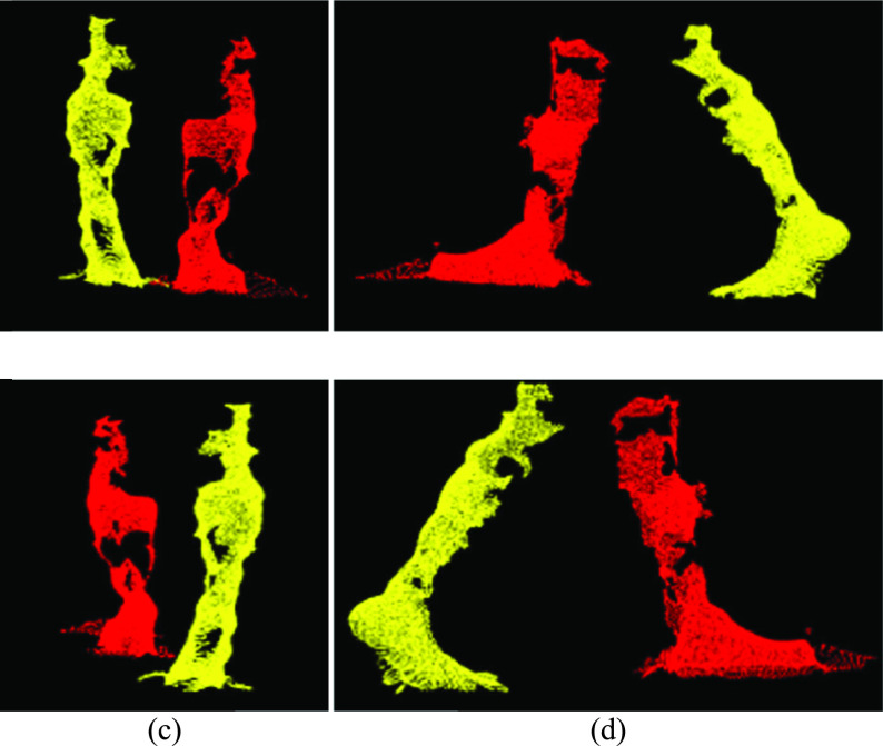
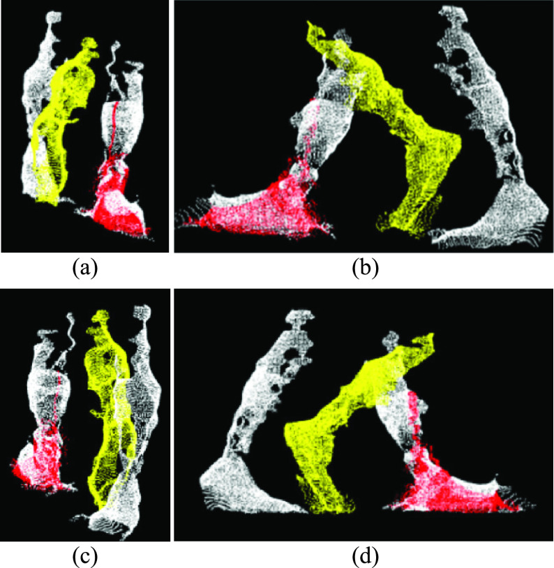
Each cluster was verified using the number of points and cluster volume (i.e., volume of the bounding box around the cluster). Point clouds with two clusters, each with a minimum of 1000 points and cluster volume greater than 75 percent of the average leg volume were considered to contain data from two legs, and each cluster was considered an individual leg (Fig. 4). Point clouds with a single cluster greater than 1000 points and volume between 0.75 to 1.25 times the average volume was considered single leg data.
FIGURE 4.
(a) Front, (b) left, (c) back, and (d) right views of the left (red) and right (yellow) leg points segmented using euclidean clustering.
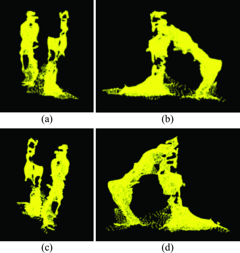
During mid-swing, when both legs are close together, noise between the legs caused the points to group into a single cluster. In these cases, the two legs data were identified as a single cluster (Fig. 5), with cluster volume greater than two times the average leg volume. Therefore, a different approach (“Moving points segmentation”) was used to segment the legs (Section IV-C).
FIGURE 5.
(a) Front, (b) left, (c) back, and (d) right views of a single clustered point cloud with two legs.
Point cloud frames not in one of these three categories (Two valid legs, single leg, two legs as a single cluster) were ignored.
B. Leg Dimensions
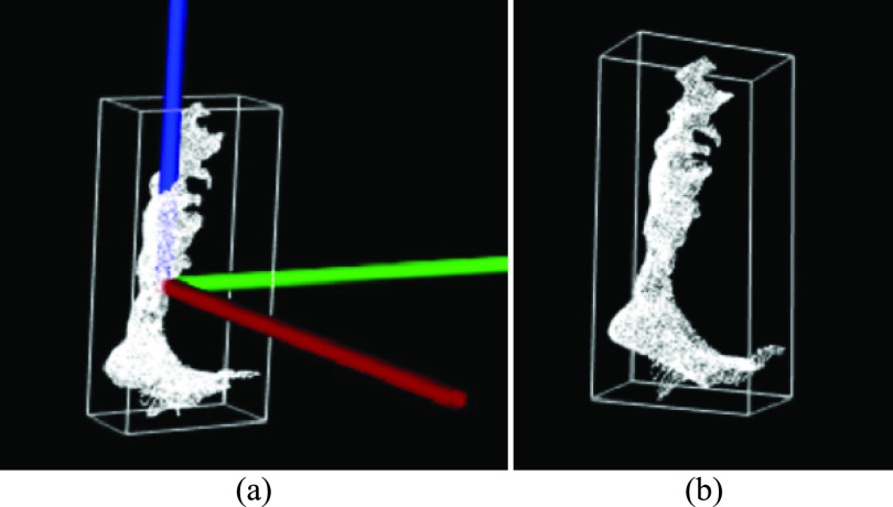
Leg dimensions were calculated from a closest oriented bounding box (OBB, Table 1) around the leg point cloud. Frames with two separate Euclidean clusters (two legs) and each leg with more than 1000 points were considered for calculating average leg dimensions, from 40 valid leg point clouds (Table 2). Dimensions ( ) were calculated using Algorithm I (Table 1) and then sorted before calculating the average of the center 20 elements for each dimension.
TABLE 1. Algorithm I: Oriented Bounding Box Around Point Cloud Data.
| Step | Methodology |
|---|---|
| 1 | Calculate the point cloud’s ( ) centroid ( ) centroid ( ) and normalized covariance matrix ( ) and normalized covariance matrix ( ). For ). For  , each covariance matrix element is divided by the number of points in the point cloud. The covariance matrix, also known as dispersion matrix, contains information on dispersion direction (Eigenvectors) and dispersion magnitude (Eigenvalues). , each covariance matrix element is divided by the number of points in the point cloud. The covariance matrix, also known as dispersion matrix, contains information on dispersion direction (Eigenvectors) and dispersion magnitude (Eigenvalues). |
| 2 | Calculate Eigenvectors ( ) for ) for  . Each vector is an OBB axis, where . Each vector is an OBB axis, where  is replaced with a cross product of is replaced with a cross product of  such that axes obey the right-hand rule. such that axes obey the right-hand rule. |
| 3 | Find an initial  transformation matrix ( transformation matrix ( ) formed using centroid and Eigenvectors as ) formed using centroid and Eigenvectors as 
|
| 4 | Find point cloud  with centroid at origin by transforming with centroid at origin by transforming  . The relation between point . The relation between point  in in  , its corresponding point , its corresponding point  in in  is is  . A transformed . A transformed  is shown in Fig. 7(a). is shown in Fig. 7(a). |
| 5 | Find the minimum ( ) and maximum ( ) and maximum ( ) of each ) of each  dimension. Obtain OBB dimensions from the absolute difference between minimum and maximum values in each dimension. dimension. Obtain OBB dimensions from the absolute difference between minimum and maximum values in each dimension. |
| 6 | Calculate OBB position ( The OBB rotation matrix is The OBB rotation matrix is  . With these dimensions, position, and rotation, an OBB around the leg point cloud can be drawn (Fig. 7(b)). . With these dimensions, position, and rotation, an OBB around the leg point cloud can be drawn (Fig. 7(b)). |
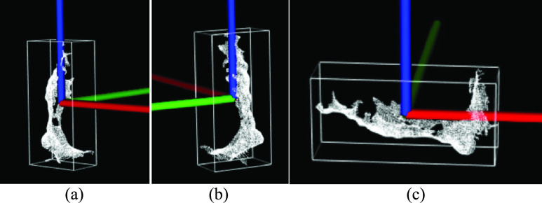
| 7 | Since rotations are not unique,  could be aligned in different ways (Fig. 8). The following steps ensure that foot AP is along the could be aligned in different ways (Fig. 8). The following steps ensure that foot AP is along the  , ML is along the , ML is along the  , and the bottom of the foot is in negative , and the bottom of the foot is in negative  . This aligned point cloud at origin is represented as . This aligned point cloud at origin is represented as  . . |
| 8 | The four closest corners to floor are considered OBB bottom corners. The rest are top corners. Any bottom corner can be considered the reference point. Distances from the reference point to the remaining three bottom corners are calculated. Minimum distance is OBB width ( ), maximum distance is diagonal, and middle distance is OBB length ( ), maximum distance is diagonal, and middle distance is OBB length ( ). The minimum distance from the reference corner to the top corners is the OBB height ( ). The minimum distance from the reference corner to the top corners is the OBB height ( ). ). |
| 9 | From a reference point, calculate a unit vector in the length direction ( ) and a unit vector in the height direction ( ) and a unit vector in the height direction ( ). ). |
| 10 | Calculate the rotation matrix ( ) between a coordinate system with point ) between a coordinate system with point  as the origin, unit vectors as the origin, unit vectors  , and , and  and the other coordinate system with corresponding values and the other coordinate system with corresponding values  and and  . This . This  is the new rotation matrix for the OBB. is the new rotation matrix for the OBB. |
TABLE 2. Algorithm II: Valid Frames to Measure Dimensions.
| Step | Methodology |
|---|---|
| 1 | Calculate  for a leg point cloud ( for a leg point cloud ( ), using Algorithm I (Table 1). ), using Algorithm I (Table 1). |
| 2 | For every point ( ) in ) in  , a corresponding point ( , a corresponding point ( ) in the point cloud ) in the point cloud  is calculated using is calculated using 
|
| 3 | A box with centroid at the origin, height ( ) in the z-axis, width ( ) in the z-axis, width ( ) in the y-axis, and length ( ) in the y-axis, and length ( ) in the x-axis bounds the ) in the x-axis bounds the  . . |
| 4 | Divide this box into 12 horizontal slices along the z-axis, starting from the bottom, with 25 mm height, length ( ), and width ( ), and width ( ). ). |
| 5 | For each slice, calculate minimum ( ) and maximum ( ) and maximum ( ) for each ) for each  dimension using points inside the slice. Calculate the slice volume as dimension using points inside the slice. Calculate the slice volume as  . . |
| 6 | A leg point cloud is considered valid for calculating dimensions if the maximum  was one of the bottom two slices and value greater than 80 percent of was one of the bottom two slices and value greater than 80 percent of  . . |
C. Moving Points Segmentation
For a current point cloud frame ( ) with two legs identified as a single cluster, a reference point cloud (
 ) from the past frames was found using Algorithm III (Table 3).
TABLE 3. Algorithm III: Past Reference Point Cloud Frame.
| Step | Methodology |
|---|---|
| 1 | Project point cloud data ( ) of the ) of the  frame onto the floor plane and calculate centroid on the floor ( frame onto the floor plane and calculate centroid on the floor ( ). ). |
| 2 | Reference frame at  and and  . . |
| 3 | If the number of points in the  frame’s point cloud is less than 1000, go to step 6. frame’s point cloud is less than 1000, go to step 6. |
| 4 | Project point cloud data at  frame onto the floor plane and calculate centroid on the floor ( frame onto the floor plane and calculate centroid on the floor ( ). ). |
| 5 |
 frame is the reference point cloud ( frame is the reference point cloud ( ), if the distance between ), if the distance between  and and  is greater than 100mm else go to the next step. is greater than 100mm else go to the next step. |
| 6 | For  ; if ; if  go to step 3, else ignore the go to step 3, else ignore the  frame. frame. |
From every point in the reference point cloud ( ), points within 20 mm in
  were categorized as the non-moving leg point cloud
  (repeated points were ignored).
All other points in  were moving points and categorized as the other leg’s point cloud
  . Each point cloud had at least 30 percent of the total points in
  and the statistical outlier removal filter was applied (Section III-D). Euclidean clustering (Section IV-A) was applied to
  and
and  , the biggest cluster from each point cloud was considered (Fig. 6).
FIGURE 7.
(a) Point cloud  with centroid at origin, (b) OBB around
  (Red:
(Red:  , Green:
  , and Blue:
  ).
).
FIGURE 8.
Leg  with AP of the foot along (a)
  (red), (b)
  (green), (c)
  (Blue).
FIGURE 6.
(a) Front, (b) left, (c) back, and (d) right views of a reference point cloud frame (white) and current point cloud frame segmented into non-moving leg points (red) and moving leg (yellow).
V. Foot Tracking
Foot tracking was achieved from point cloud data by fitting a box with average foot dimensions around each foot, in each frame. The foot’s bottom plane was calculated and used to define bounding box rotation and position. The foot’s heel and toe points were based on the walking direction.
A. Foot Dimensions
Using Algorithm II (Table 2), for a valid frame, the volume of points in 12 slices were calculated. Each slice’s volume was median filtered with both adjacent slice volumes using filter size = 3 and filter stride length = 1 (first and last elements were untouched).
The cut-off slice (i.e., slice defining top of foot) was defined by identifying the slice with the maximum volume ( ) and then scanning upwards to find the slice with volume less than 60 percent of
  . The points below this cut-off slice defined the foot. An OBB was calculated around these points (Table 1, Algorithm I) and OBB dimensions were foot length (
 foot width (
 ), and foot height (
 ). These dimensions were found for 40 frames, values of each dimension were sorted and the center 20 elements were averaged.
B. Foot Oriented Bounding Box
The foot’s bottom plane was found using Algorithm IV (Table 4). Points above this plane within the distance  were considered to belong to foot point cloud (
 ) and points between 0.1 times
  and 0.9 times
  were segmented as the center foot’s point cloud (
 ).
).
TABLE 4. Algorithm IV: Foot Bottom Plane.
| Step | Methodology |
|---|---|
| 1 | Apply Algorithm I to a leg point cloud ( ) and align the outputs at origin ( ) and align the outputs at origin ( ), OBB position ( ), OBB position ( ), rotation ( ), rotation ( ), length ( ), length ( ), width ( ), width ( ), and height ( ), and height ( ). ). |
| 2 | From an OBB bottom corner around  , five sub-boxes with length ( , five sub-boxes with length ( ), width ( ), width ( ), and height ( ), and height ( ) are taken. The two outer bottom corner points of the first sub-box from the bottom, with a minimum of 50 points, are transformed using ) are taken. The two outer bottom corner points of the first sub-box from the bottom, with a minimum of 50 points, are transformed using  and and  . These transformed points ( . These transformed points ( ) are the foot OBB corners. ) are the foot OBB corners. |
| 3 | Repeat step 2 for the foot’s other side. |
| 4 | From a point  , the centroid of thirty closest points in , the centroid of thirty closest points in  is considered the foot bottom point ( is considered the foot bottom point ( ). Repeat to find all the four bottom points on the foot. ). Repeat to find all the four bottom points on the foot. |
| 5 | Using these four  points, four plane equations are obtained by taking different combinations of three points and distance from the fourth point to the plane is calculated. The plane with the smallest distance from the fourth point is the “Best Plane”. points, four plane equations are obtained by taking different combinations of three points and distance from the fourth point to the plane is calculated. The plane with the smallest distance from the fourth point is the “Best Plane”. |
| 6 | Points within 5 mm above the best plane are fitted to a RANSAC plane model [30] and the output considered as foot’s bottom plane. |
 points were projected onto the foot’s bottom plane and then Algorithm I was partially applied (until step 6). OBB rotation around the foot (
 ) was obtained with dimensions (
 ). Then OBB dimensions mapped with average foot dimensions as the minimum of
  were replaced with
  , maximum with
  , and the remaining dimension with
  .
.
The foot’s OBB position ( ) was the centroid of
  . Position (
 ), rotation (
 ), and dimensions (
 ) were used to locate a box around the foot.
C. Heel and Toe Segmentation
The point cloud data was transformed using 5000 mm translations in the  and
and  axes such that the walking pathway was always in the positive xy-plane. This reduced the complexity of further processing and understanding.
Left and right leg segmentation was based on the walking direction, calculated using OBB centroid trajectory. When walking towards the origin along a pathway parallel to the  -axis, the leg closer to the
  -axis was the right leg and the other leg was labelled as left. Opposite leg classification was applied when walking away from the origin.
For each foot OBB, the center point ( ) of the front two bottom corners and the center point (
 ) of the back two bottom corners were calculated using Algorithm V (Table 5). These points were considered as the toe and heel, respectively (Fig. 9).
TABLE 5. Algorithm V: Heel and Toe Segmentation.
| Step | Methodology |
|---|---|
| 1 | Calculate OBB centroid ( ). ). |
| 2 | Identify OBB four front corners and four back corners. 
|
| 3 | Calculate centroid of front corners ( ) and back corners ( ) and back corners ( ). ). |
| 4 | From front corners, front left and front right corners are: 
|
| 5 | From back corners, back left and back right corners are: 
|
| 6 | For front, the front left bottom corner has a lower z-axis value and the other is the front left top corner. The same logic is applied to front right corners, back left corners, and back right corners. |
| 7 | Calculate foot length, width, and height and validated with average foot dimensions ( ). ). 
|
| 8 | OBB toe point is the center of front bottom two points ( ) and heel point is the center of back bottom two points ( ) and heel point is the center of back bottom two points ( ). ). |
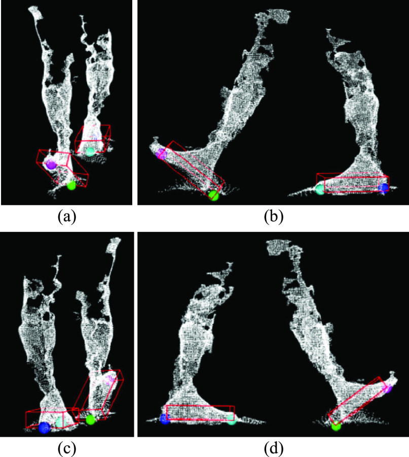
FIGURE 9.
(a) Front, (b) left, (c) back, and (d) right views of a point cloud frame with heel and toe segmentation (right heel – green, right toe – magenta, left heel – blue, left toe – cyan).
VI. Validation
The foot tracking algorithm was validated by comparing gold standard Vicon system output with the marker-less smart hallway system. Volunteer walking trials were captured simultaneously with both the systems and post-processing filters were applied. This section describes the data collection protocol and post-processing processes.
A. Protocol
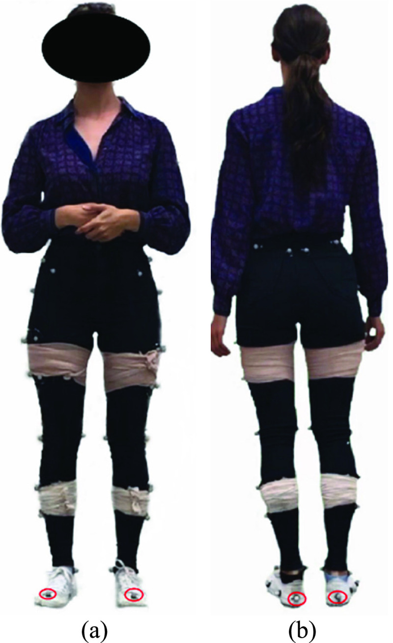
Twenty-two able-bodied volunteers were recruited from students and staff at the University of Ottawa. After informed consent, reflective markers were attached to the participant’s lower body (Fig. 10) (foot markers were used in this application) and then the participant walked 12 times with their natural gait and comfortable speed along a walkway with a 1.5m capture zone. Data were captured simultaneously with a 13 camera Vicon system at 100 Hz [31] and the new marker-less system at approximately 60 Hz. Since the Vicon system captured more than the 1.5m walkway, the data within the capture zone of both systems were used for calculating the stride parameters. This protocol was approved by the Research Ethics Board of the University of Ottawa (File number: H-08-18-860, Approval date: 29-10-2018) [32].
FIGURE 10.
(a) Front and (b) back view of a participant with reflective markers.
In this study, Vicon and the new marker-less system were not synchronized in time. Even though both systems captured data simultaneously, each system was independent. Stride parameters were calculated individually, then synchronized based on spatial foot events information.
B. Post-Processing
3D positions of left toe, left heel, right toe, and right heel markers were reconstructed using Vicon Nexus software [33]. Gaps in the trial data were filled using cubic spline interpolation and then filtered using a 4th order dual-pass Butterworth lowpass filter with 20 Hz cut-off frequency.
Marker-less point cloud data were constructed from the depth images, then 3D locations of toes and heels were tracked. Left toe, left heel, right toe, and right heel were processed independently. Data outliers were statistically filtered, with values two standard deviations or more from the mean removed. Based on time stamp information, trajectory gaps were filled using cubic spline interpolation.
Since the capture time between frames was inconsistent, cubic spline interpolation was used to re-sample the data to 60Hz. This re-sampled data was low pass filtered using 4th order dual-pass Butterworth filter with a cut-off frequency of 12Hz. Using cubic spline interpolation, the low pass filtered data was then re-sampled gain to the originally captured time stamps.
VII. Stride Parameters
This section describes the stride parameters used with both Vicon and marker less systems. The stride parameters were calculated by finding the foot events from the segmented heel and toe points obtained from the foot-tracking algorithm.
Foot events such as foot strike (FS) and foot-off (FO) were identified to calculate stride parameters. Vertical foot coordinates ( -axis) were used to identify FS and FO frames [34].
A. Foot Events
1). VICON
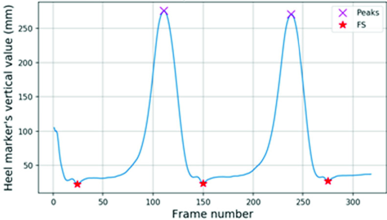
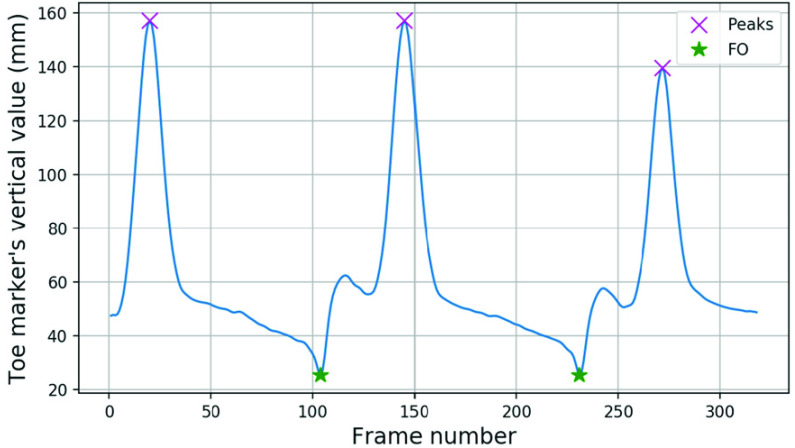
Peak vertical values in swing phase were detected for heel (Fig. 11) and toe (Fig. 12) markers. These peaks were based on the zero cross over from positive to negative in the vertical velocity, then a peak value greater than 75 percent of the maximum vertical value condition was applied.
FIGURE 11.
FS events from the Vicon heel marker’s vertical values.
FIGURE 12.
FO events from the Vicon toe marker’s vertical values.
Between two peaks, FS and FO should only occur once. Zero crossovers from negative to positive in the vertical velocity were concave shaped dips in the vertical displacement graph. These concave dips within the bottom 20 percent of the vertical range were identified. The FS frame was the minimum dip between the two peaks in heel data (Fig. 11) and FO was the minimum dip in toe data (Fig. 12).
Additional conditions were applied to the minimum concave dips before the first peak and after the last peak. The minimum concave dip before the first peak with a distance (in frames) less than 50 percent of the frame length between the first two heel peaks was ignored, and greater than 50 percent in the toe data was ignored. Similarly, the number of frames between the last peak and the minimum concave dip after the last peak must be less than 50 percent of the frame length between the last two peaks for heel data and greater than 50 percent for toe data.
2). Marker-Less
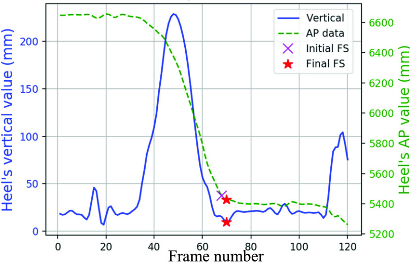
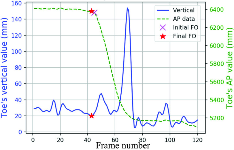
Vertical direction data from the Marker-less system was not as smooth as the Vicon data. The foot event frames were initially estimated using AP (y-axis) data, then finalized based on the vertical data.
The frame where the foot reached a stationary state in the AP direction was considered the initial FS frame (Fig. 13). Vertical movements may occur after AP movements halted, so the closest concave dip within the next five frames in vertical data was considered as the final FS (Fig. 13). For cases with no concave dip, the initially estimated frame was considered the final FS. The final FO frame was determined from an initially estimated FO frame, where AP displacement began (Fig. 14), and five frames before the initial estimated FO frame in the vertical direction (Fig. 14). This method is detailed in Algorithm VI (Table 6).
FIGURE 13.
FS events in marker-less system’s heel data.
FIGURE 14.
FO events in marker-less system’s toe data.
TABLE 6. Algorithm VI: Foot Events Identification in the Marker-Less Data.
| Step | Methodology |
|---|---|
| 1 | Create a binary version of arrays for  heel data ( heel data ( ) and ) and  toe data ( toe data ( ). For ). For  data ( data ( ) with ) with  frames, the frames, the  frame in binary version ( frame in binary version ( ) is calculated as ) is calculated as 
|
| 2 | Median filter binary arrays with filter size = 3 and filter stride = 1. |
| 3 | In the sequence of binary heel frames, the transition frame from high to low with at least three high-valued frames and two low-valued frames is the initial FS frame. |
| 4 | The closest zero cross-over frame from negative to positive in the heel’s vertical velocity within the next five frames after the initial FS frame is the final FS frame. If no such frame exists, then initial and final FS frame are the same. |
| 5 | In the sequence of binary toe frames, the transition frame from low to high with at least three low-valued frames and two high-valued frames is the initial FO frame. |
| 6 | The closest zero cross over frame from negative to positive in the toe’s vertical velocity within the before five frames of the initial FO frame is the final FO frame. If no such frame exists, then the initial and final FS frame are the same. |
Left Foot Strike (LFS), Left Foot-Off (LFO), Right Foot Strike (RFS), and Right Foot-off (RFO) were validated according to the normal gait cycle event sequence (i.e., after LFO, the expected next event is LFS and then RFO). If multiple LFS events are identified before RFO, the closest to the RFO event was considered. If no LFS event was identified between LFO and RFO, then the events were ignored.
B. Results
The stride parameters in this research were from one gait cycle (Table 7). Primary parameters were directly obtained from the tracking data and the derived parameters were calculated from the primary parameters.
TABLE 7. Stride Parameters Calculations in a Normal Gait Cycle.
| Parameter | Definition |
|---|---|
| Left stride length | Distance covered by the left heel between two consecutive LFS along the sagittal plane (line of progression,  ) ) |
| Right stride length | Sagittal distance covered by the right heel between two consecutive RFS |
| Left stride time | Time between two consecutive LFS |
| Right stride time | Time between two consecutive RFS |
| Left stride speedd | Left stride length / Left stride time |
| Right stride speedd | Right stride length / Right stride time |
| Left step length | Sagittal distance between right and left heels at LFS |
| Left step width | Frontal distance ( ) between right and left heels at LFS ) between right and left heels at LFS |
| Left step time | Time between RFS and LFS |
| Right step length | Sagittal distance between left and right heels at RFS |
| Right step width | Frontal distance between left and right heels at RFS |
| Right step time | Time between LFS and RFS |
| Left cadenced | Left steps per minute |
| Right cadenced | Right steps per minute |
| Left stance time | Time between LFS and LFO |
| Left swing time | Time between LFO and LFS |
| Left stance to swing ratiod | Left stance time / Left swing time |
| Right stance to swing ratiod | Right stance time / Right swing time |
| Left double support time | Time between LFS and RFO |
| Right double support time | Time between RFS and LFO |
| Left foot angle | Angle of left foot midline with sagittal plane when the left foot is entirely in contact with the floor. |
| Right foot angle | Angle of right foot midline with sagittal when the right foot is entirely in contact with the floor. |
| Left foot maximum velocity | Maximum left foot velocity during the left swing phase (LFO to LFS) |
| Right foot maximum velocity | Maximum right foot velocity during the right swing phase (RFO to RFS) |
| Left foot clearance | Minimum vertical distance of left foot during mid-swing |
| Right foot clearance | Minimum vertical distance of right foot during its mid-swing |
Derived stride parameters
Foot events from Vicon and marker-less systems were synced based on foot position of the first common foot event in the marker-less system.
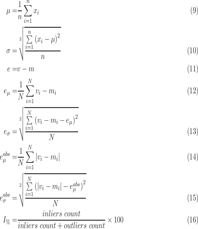
Stride parameters from the both systems were compared and analyzed. For  samples, with
  sample represented as
  , the mean (
 ) and standard deviation (
 ) were calculated using (9) and (10), respectively. For a parameter, with value
  from the Vicon system and value
  from marker-less system, the sample error (
 ) was calculated using (11).
For each primary stride parameter,  and
and  of the error values were calculated. Most values farther than two
  from the
  were due to false detection of foot events because of insufficient capturing volume and noisy data. Since these erroneous data was not because of improper foot tracking, it was categorized as outliers and removed from the analysis. Primary stride parameter inliers were used to calculate derived stride parameters. For a stride parameter with
  samples (inliers),
  Vicon’s sample
  ,
,  marker-less system’s sample
  , the mean error (
 ), error’s standard deviation (
 ), absolute mean error (
 ), absolute error’s standard deviation (
 ), minimum error (
 ), maximum error (
 ), Pearson coefficient (
 ), and the percentage of inliers (
 ) were calculated (Table 8).
TABLE 8. Marker-Less Stride Analysis.
| Parameter (units) | Vicon ( ) ) |
Marker-less ( ) ) |
Error ( ) ) |
 |
 |
 |
 |
Inliers count |  |
|
|---|---|---|---|---|---|---|---|---|---|---|
| Left | Stride speed (m/s) | 1.06 ± 0.11 | 1.05 ± 0.11 | 0.012 ± 0.02 | 0.018 ± 0.02 | −0.03 | 0.07 | 0.98 | – | – |
| Stride length (m) | 1.29 ± 0.09 | 1.28 ± 0.09 | 0.012 ± 0.03 | 0.023 ± 0.02 | −0.05 | 0.12 | 0.95 | 90 | 97.8 | |
| Stride time (s) | 1.22 ± 0.09 | 1.23 ± 0.1 | −0.002 ± 0.04 | 0.027 ± 0.02 | −0.10 | 0.11 | 0.93 | 87 | 94.5 | |
| Cadence (steps/min) | 100.95 ± 8.5 | 100.79 ± 9.29 | 0.159 ± 5.35 | 4.043 ± 3.51 | −22.22 | 15.48 | 0.82 | – | – | |
| Step length (cm) | 66.32 ± 5.14 | 66.07 ± 5.52 | 0.247 ± 2.45 | 1.825 ± 1.66 | −13.46 | 8.93 | 0.90 | 207 | 92.0 | |
| Step width (cm) | 9.65 ± 4.06 | 7.24 ± 4.4 | 2.415 ± 2.64 | 2.986 ± 1.97 | −5.28 | 8.74 | 0.81 | 213 | 94.6 | |
| Step time (s) | 0.6 ± 0.05 | 0.60 ± 0.06 | −0.002 ± 0.03 | 0.024 ± 0.02 | −0.10 | 0.10 | 0.85 | 221 | 98.2 | |
| Stance time (s) | 0.78 ± 0.07 | 0.79 ± 0.08 | −0.008 ± 0.03 | 0.024 ± 0.02 | −0.10 | 0.07 | 0.92 | 185 | 97.8 | |
| Swing time (s) | 0.42 ± 0.04 | 0.43 ± 0.04 | −0.003 ± 0.03 | 0.028 ± 0.02 | −0.08 | 0.08 | 0.60 | 173 | 96.6 | |
| Stance to swing ratio (NA) | 1.86 ± 0.14 | 1.90 ± 0.22 | −0.031 ± 0.21 | 0.172 ± 0.12 | −0.67 | 0.38 | 0.41 | – | – | |
| Double support time (s) | 0.17 ± 0.03 | 0.18 ± 0.04 | −0.004 ± 0.03 | 0.027 ± 0.02 | −0.11 | 0.10 | 0.53 | 248 | 98.4 | |
| Foot angle (°) | 8.34 ± 5.14 | 1.12 ± 0.63 | 7.209 ± 5.13 | 7.256 ± 5.06 | −1.22 | 19.14 | 0.08 | 176 | 93.6 | |
| Foot max. velocity(m/s) | 3.71 ± 0.31 | 3.88 ± 0.37 | −0.163 ± 0.28 | 0.247 ± 0.22 | −1.01 | 0.45 | 0.66 | 171 | 95.5 | |
| Foot clearance (cm) | 2.6 ± 0.62 | 1.99 ± 1.36 | 0.605 ± 1.39 | 1.224 ± 0.90 | −4.19 | 3.07 | 0.18 | 113 | 93.4 | |
| Right | Stride speed (m/s) | 1.1 ± 0.12 | 1.09 ± 0.12 | 0.006 ± 0.02 | 0.017 ± 0.01 | 0.06 | −0.04 | 0.98 | – | – |
| Stride length (m) | 1.29 ± 0.10 | 1.29 ± 0.10 | 0.001 ± 0.02 | 0.017 ± 0.01 | 0.06 | −0.04 | 0.97 | 79 | 96.3 | |
| Stride time (s) | 1.19 ± 0.09 | 1.19 ± 0.09 | −0.007 ± 0.03 | 0.025 ± 0.02 | 0.08 | −0.07 | 0.95 | 77 | 93.9 | |
| Cadence (steps/min) | 99.44 ± 7.55 | 99.28 ± 7.95 | 0.157 ± 4.68 | 3.678 ± 2.89 | 12.7 | −12.72 | 0.82 | – | – | |
| Step length (cm) | 64.80 ± 4.96 | 64.42 ± 5.41 | 0.3767 ± 2.19 | 1.722 ± 1.40 | 8.25 | −8.82 | 0.91 | 177 | 89.8 | |
| Step width (cm) | 9.54 ± 3.76 | 6.80 ± 4.30 | 2.742 ± 2.75 | 3.227 ± 2.16 | 8.86 | −5.19 | 0.77 | 185 | 93.9 | |
| Step time (s) | 0.61 ± 0.05 | 0.61 ± 0.05 | −0.001 ± 0.03 | 0.023 ± 0.02 | 0.10 | −0.08 | 0.82 | 193 | 97.9 | |
| Stance time. (s) | 0.77 ± 0.07 | 0.78 ± 0.08 | −0.009 ± 0.03 | 0.025 ± 0.02 | 0.08 | −0.10 | 0.92 | 206 | 98.5 | |
| Swing time. (s) | 0.43 ± 0.03 | 0.42 ± 0.04 | 0.003 ± 0.03 | 0.023 ± 0.02 | 0.08 | −0.06 | 0.69 | 141 | 94.6 | |
| Stance to swing (NA) | 1.82 ± 0.13 | 1.85 ± 0.18 | −0.027 ± 0.15 | 0.127 ± 0.09 | 0.38 | −0.36 | 0.56 | – | – | |
| Double support (s) | 0.17 ± 0.03 | 0.17 ± 0.05 | −0.002 ± 0.04 | 0.027 ± 0.02 | 0.10 | −0.16 | 0.65 | 245 | 99.6 | |
| Foot angle (°) | 9.05 ± 5.71 | 1.14 ± 0.58 | 7.915 ± 5.62 | 7.935 ± 5.60 | 21.21 | −0.92 | 0.20 | 201 | 96.2 | |
| Foot max. velocity (m/s) | 3.67 ± 0.28 | 3.83 ± 0.36 | −0.155 ± 0.25 | 0.204 ± 0.21 | 0.32 | −1.07 | 0.73 | 139 | 93.3 | |
| Foot clearance (cm) | 2.68 ± 0.62 | 2.10 ± 1.44 | 0.572 ± 1.35 | 1.251 ± 0.77 | 3.26 | −3.35 | 0.36 | 102 | 96.2 | |
The mean and absolute errors for step length and step time were within the minimum detectable change (MDC) for older people (age; mean = 78.09, standard deviation = 6.2) (step length MDC95 = 47 mm, step time MDC95 = 42 ms). However, step width was slightly greater than MDC (left step width mean error = 24.15 mm, left step width absolute error = 29.86 mm, right step width mean error = 27.42 mm, right step width absolute mean error = 32.27 mm, step width for older people MDC95 = 20 mm) [35]. The best Pearson correlation coefficient was for stride speed ( ) and lower values were obtained for left foot angle (
 ) and left foot clearance (
 ).
).
C. Discussion
The novel smart hallway system successfully tracked the foot and provided viable stride parameter output that could be used for decision-making, in most cases. The marker-less system had small mean absolute errors for the majority of stride parameters, compared with the Vicon system. For all the parameters, greater than 90% were inliers. Most outliers were due to limitations of capturing zone and noise from the sensors.
To the best of our knowledge, this research is the first to report foot clearance with marker-less depth sensors. A maximum absolute mean error of 1.25 cm was observed for right foot clearance, which was too large for clinical assessment purposes. With a marker-less system frame rate at approximately 60fps, all temporal stride parameters were accurate within 10 ms mean error and 30 ms absolute mean error. Errors in spatial stride parameters were due to “floor-plane to foot plantar surface” noise generated in the depth images during foot contact phases.
In comparison to the Kinect V2 based studies [16], [17], while mean errors of walking speed, stride length, and step length parameters were in similar range, step width mean errors were high, and temporal parameters’ mean errors (step time and stride time) showed better accuracy.
The new foot tracking algorithm, based on the fixed size OBB and foot bottom plane to define foot orientation, counteracted the AP noise to some extent. Average errors were higher in ML dependent stride parameters such as step width and foot angle.
Based on the errors and comparison with the MDC for older people [35], this novel marker-less system has potential to perform stride analysis on large population of older people in institutional hallways. This novel foot tracking algorithm could obtain more accurate stride parameters with better (less noisy) point cloud data.
 |
VIII. Conclusion
In this research, we proposed a smart hallway using depth sensors for foot tracking and stride parameter analysis. With six temporally and spatially synchronized Intel RealSense D415 depth sensors, depth data were successfully background-subtracted and merged to form a walking human’s point cloud time series. The point cloud was then effectively segmented into left and right foot point clouds. A bounding box was fitted around the foot in each leg’s point cloud data. The bounding box around the foot in each frame enabled foot tracking, and stride parameter calculation. Most stride parameters obtained from this newly developed marker-less system comparable favorably with gold standard Vicon system output.
While the marker-less system had promising results with accurate temporal stride parameters and small errors in spatial stride parameters, step width accuracy needs to improve and poor foot angle accuracy was observed due to noise around the foot as it approached the floor plane. Since foot clearance error was greater than 1 cm, and foot clearance varying between 2 and 3.2 cm, this error would need to be reduced to provide usable results for clinical decision-making.
Unlike the machine learning based skeleton tracking systems, foot landmarks from our proposed system never move outside the foot and data are captured at approximately 60 fps. This system could monitor a large number of people for long hours with no preparation time (no sensors attached to the body), without any discomfort, and without expert intervention.
Acknowledgment
The authors would like to thank The Ottawa Hospital Rehabilitation Centre for providing resources for development and preliminary testing, University of Ottawa METRICS laboratory for computation facilities, and Prof. Julie Nantel and her staff for motion capture support. They would also like to thank all volunteers who participated in this study.
Funding Statement
This work was part of the CREATE-BEST program funded by the Natural Sciences and Engineering Research Council of Canada (NSERC).
References
- [1].Ferreira J. P., Crisostomo M. M., and Coimbra A. P., “Human gait acquisition and characterization,” IEEE Trans. Instrum. Meas., vol. 58, no. 9, pp. 2979–2988, Sep. 2009, doi: 10.1109/TIM.2009.2016801. [DOI] [Google Scholar]
- [2].Robert-Lachaine X., Mecheri H., Larue C., and Plamondon A., “Validation of inertial measurement units with an optoelectronic system for whole-body motion analysis,” Med. Biol. Eng. Comput., vol. 55, no. 4, pp. 609–619, Apr. 2017, doi: 10.1007/s11517-016-1537-2. [DOI] [PubMed] [Google Scholar]
- [3].Patterson M. R.et al. , “Does external walking environment affect gait patterns?,” in Proc. 36th Annu. Int. Conf. IEEE Eng. Med. Biol. Soc., Aug. 2014, pp. 2981–2984, doi: 10.1109/EMBC.2014.6944249. [DOI] [PubMed] [Google Scholar]
- [4].Stone E. E. and Skubic M., “Passive in-home measurement of stride-to-stride gait variability comparing vision and Kinect sensing,” in Proc. Annu. Int. Conf. IEEE Eng. Med. Biol. Soc., Aug. 2011, pp. 6491–6494, doi: 10.1109/IEMBS.2011.6091602. [DOI] [PubMed] [Google Scholar]
- [5].Nizam Y., Mohd M. N., and Jamil M. M. A., “Biomechanical application: Exploitation of Kinect sensor for gait analysis,” ARPN J. Eng. Appl. Sci., vol. 12, no. 10, pp. 3183–3188, 2017. [Google Scholar]
- [6].Dubois A. and Charpillet F., “A gait analysis method based on a depth camera for fall prevention,” in Proc. 36th Annu. Int. Conf. IEEE Eng. Med. Biol. Soc., Aug. 2014, pp. 4515–4518, doi: 10.1109/EMBC.2014.6944627. [DOI] [PubMed] [Google Scholar]
- [7].Procházka A., Vyšata O., Vališ M., Ťupa O., Schätz M., and Mařík V., “Use of the image and depth sensors of the microsoft kinect for the detection of gait disorders,” Neural Comput. Appl., vol. 26, no. 7, pp. 1621–1629, Oct. 2015, doi: 10.1007/s00521-015-1827-x. [DOI] [Google Scholar]
- [8].Newland P., Wagner J. M., Salter A., Thomas F. P., Skubic M., and Rantz M., “Exploring the feasibility and acceptability of sensor monitoring of gait and falls in the homes of persons with multiple sclerosis,” Gait Posture, vol. 49, pp. 277–282, Sep. 2016, doi: 10.1016/j.gaitpost.2016.07.005. [DOI] [PubMed] [Google Scholar]
- [9].Kamthan P., “Tip-toe walking detection using CPG parameters from skeleton data gathered by Kinect,” in Proc. 11th Int. Conf. Ubiquitous Comput. Ambient Intell., vol. 2, 2017, pp. 79–90, doi: 10.1007/978-3-319-67585-5. [DOI] [Google Scholar]
- [10].Zhao J., Bunn F. E., Perron J. M., Shen E., and Allison R. S., “Gait assessment using the Kinect RGB-D sensor,” in Proc. 37th Annu. Int. Conf. IEEE Eng. Med. Biol. Soc. (EMBC), Aug. 2015, pp. 6679–6683, doi: 10.1109/EMBC.2015.7319925. [DOI] [PubMed] [Google Scholar]
- [11].Dao N.-L., Zhang Y., Zheng J., and Cai J., “Kinect-based non-intrusive human gait analysis and visualization,” in Proc. IEEE 17th Int. Workshop Multimedia Signal Process. (MMSP), Oct. 2015, pp. 1–6, doi: 10.1109/MMSP.2015.7340804. [DOI] [Google Scholar]
- [12].Paolini G.et al. , “Validation of a method for real time foot position and orientation tracking with microsoft kinect technology for use in virtual reality and treadmill based gait training programs,” IEEE Trans. Neural Syst. Rehabil. Eng., vol. 22, no. 5, pp. 997–1002, Sep. 2014, doi: 10.1109/TNSRE.2013.2282868. [DOI] [PubMed] [Google Scholar]
- [13].Gabel M., Gilad-Bachrach R., Renshaw E., and Schuster A., “Full body gait analysis with kinect,” in Proc. Annu. Int. Conf. IEEE Eng. Med. Biol. Soc., Aug. 2012, pp. 1964–1967, doi: 10.1109/EMBC.2012.6346340. [DOI] [PubMed] [Google Scholar]
- [14].Goncalves R. S., Hamilton T., and Krebs H. I., “MIT-skywalker: On the use of a markerless system,” in Proc. Int. Conf. Rehabil. Robot. (ICORR), Jul. 2017, pp. 205–210, doi: 10.1109/ICORR.2017.8009247. [DOI] [PubMed] [Google Scholar]
- [15].Kharazi M. R.et al. , “Validity of microsoft kinectTM for measuring gait parameters,” in Proc. 22nd Iranian Conf. Biomed. Eng. (ICBME), Nov. 2015, pp. 375–379, doi: 10.1109/ICBME.2015.7404173. [DOI] [Google Scholar]
- [16].Geerse D. J., Coolen B. H., and Roerdink M., “Kinematic validation of a multi-Kinect V2 instrumented 10-meter walkway for quantitative gait assessments,” PLoS ONE, vol. 10, no. 10, pp. 1–15, 2015, doi: 10.1371/journal.pone.0139913. [DOI] [PMC free article] [PubMed] [Google Scholar]
- [17].Müller B., Ilg W., Giese M. A., and Ludolph N., “Validation of enhanced Kinect sensor based motion capturing for gait assessment,” PLoS ONE, vol. 12, no. 4, pp. 14–16, 2017, doi: 10.1371/journal.pone.0175813. [DOI] [PMC free article] [PubMed] [Google Scholar]
- [18].Colley J., Zeeman H., and Kendall E., “‘Everything happens in the hallways’: Exploring user activity in the corridors at two rehabilitation units,” HERD, Health Environ. Res. Design J., vol. 11, no. 2, pp. 163–176, Apr. 2018, doi: 10.1177/1937586717733149. [DOI] [PubMed] [Google Scholar]
- [19].Gutta V., Lemaire E. D., Baddour N., and Fallavollita P., “A comparison of depth sensors for 3D object surface reconstruction,” CMBES Proc., vol. 42, May 2019. [Online]. Available: https://proceedings.cmbes.ca/index.php/proceedings/article/view/881 [Google Scholar]
- [20].Gutta V., Baddour N., Fallavollita P., and Lemaire E. D., “Multiple depth sensor setup and synchronization for marker-less 3D human foot tracking in a hallway,” in Proc. IEEE/ACM 1st Int. Workshop Softw. Eng. Healthcare (SEH), May 2019, pp. 77–80, doi: 10.1109/SEH.2019.00021. [DOI] [Google Scholar]
- [21].Intel RealSense D4xx Post Processing. Accessed: Jan. 30, 2019. [Online]. Available: https://www.intel.com/content/dam/support/us/en/documents/emerging-technologies/intel-realsense-technology/Intel-RealSense-Depth-PostProcess.pdf
- [22].Stone E. and Skubic M., “Evaluation of an inexpensive depth camera for passive in-home fall risk assessment,” in Proc. 5th Int. ICST Conf. Pervasive Comput. Technol. Healthcare, 2011, pp. 71–77, doi: 10.4108/icst.pervasivehealth.2011.246034. [DOI] [Google Scholar]
- [23].Grana C., Borghesani D., and Cucchiara R., “Decision trees for fast thinning algorithms,” in Proc. Int. Conf. Pattern Recognit., vol. 19, no. 6, 2010, pp. 2836–2839, doi: 10.1109/ICPR.2010.695. [DOI] [Google Scholar]
- [24].Rusu R. B., Marton Z. C., Blodow N., Dolha M., and Beetz M., “Towards 3D point cloud based object maps for household environments,” Robot. Auto. Syst., vol. 56, no. 11, pp. 927–941, Nov. 2008, doi: 10.1016/j.robot.2008.08.005. [DOI] [Google Scholar]
- [25].Alexa M., Behr J., Cohen-Or D., Fleishman S., Levin D., and Silva C. T., “Computing and rendering point set surfaces,” IEEE Trans. Vis. Comput. Graphics, vol. 9, no. 1, pp. 3–15, Jan. 2003, doi: 10.1109/TVCG.2003.1175093. [DOI] [Google Scholar]
- [26].Voxel Grid Filter. Accessed: Jan. 30, 2019. [Online]. Available: http://docs.pointclouds.org/1.8.1/classpcl_1_1_voxel_grid.html
- [27].OpenCV. Accessed: Oct. 2, 2019. [Online]. Available: http://www.opencv.org
- [28].PCL. Accessed: Oct. 2, 2019. [Online]. Available: http://www.pointclouds.org
- [29].Rusu R. B., Semantic 3D Object Maps for Everyday Manipulation in Human Living Environments. Munich, Germany: Technischen Universität München, 2009. [Google Scholar]
- [30].Fischler M. A. and Bolles R. C., “Random sample consensus: A paradigm for model fitting with applications to image analysis and automated cartography,” Commun. ACM, vol. 24, no. 6, pp. 381–395, Jun. 1981. [Google Scholar]
- [31].Vicon. Accessed: Oct. 17, 2019. [Online]. Available: http://www.vicon.com
- [32].Research Ethics Board. Accessed: Oct. 17, 2019. [Online]. Available: http://www.research.uottawa.ca/ethics/
- [33].Nexus. Accessed: Oct. 17, 2019. [Online]. Available: https://www.vicon.com/software/nexus/
- [34].Sinclair J., Edmundson C., Brooks D., and Hobbs S., “Evaluation of kinematic methods of identifying gait events during running,” Int. J. Sport., vol. 5, no. 3, pp. 188–192, 2011. [Google Scholar]
- [35].Wroblewska L.et al. , “The test-retest reliability and minimal detectable change of spatial and temporal gait variability during usual over-ground walking for younger and older adults,” Gait Posture, vol. 33, no. 8, pp. 839–841, 2016, doi: 10.1016/j.gaitpost.2015.11.014. [DOI] [PMC free article] [PubMed] [Google Scholar]


