A Physiologically Based Pharmacokinetic Model for Naphthalene With Inhalation and Skin Routes of Exposure

Abstract

Naphthalene, a volatile organic compound present in moth repellants and petroleum-based fuels, has been shown to induce toxicity in mice and rats during chronic inhalation exposures. Although simpler default methods exist for extrapolating toxicity points of departure from animals to humans, using a physiologically based pharmacokinetic (PBPK) model to perform such extrapolations is generally preferred. Confidence in PBPK models increases when they have been validated using both animal and human in vivo pharmacokinetic (PK) data. A published inhalation PBPK model for naphthalene was previously shown to predict rodent PK data well, so we sought to evaluate this model using human PK data. The most reliable human data available come from a controlled skin exposure study, but the inhalation PBPK model does not include a skin exposure route; therefore, we extended the model by incorporating compartments representing the stratum corneum and the viable epidermis and parameters that determine absorption and rate of transport through the skin. The human data revealed measurable blood concentrations of naphthalene present in the subjects prior to skin exposure, so we also introduced a continuous dose-rate parameter to account for these baseline blood concentration levels. We calibrated the three new parameters in the modified PBPK model using data from the controlled skin exposure study but did not modify values for any other parameters. Model predictions then fell within a factor of 2 of most (96%) of the human PK observations, demonstrating that this model can accurately predict internal doses of naphthalene and is thus a viable tool for use in human health risk assessment.

Naphthalene, a volatile organic compound found in moth repellants and petroleum-based fuels, has been shown to induce respiratory tract toxicity in both mice and rats during chronic inhalation exposures (NTP, 1992, 2000). Two-year inhalation studies demonstrated carcinogenicity in the form of increased incidence of nasal respiratory epithelium adenomas in male rats and olfactory epithelial neuroblastomas in female rats (Abdo et al., 2001; NTP, 2000) and alveolar/bronchiolar adenomas and carcinomas in female mice (Abdo et al., 1992; NTP, 1992). Metabolism of naphthalene by enzymes, notably CYP2F isoforms (Baldwin et al., 2004; Bogen et al., 2008), yields reactive metabolites that may be responsible for carcinogenesis, muta-genesis, and cytotoxicity (Buckpitt et al., 2002; Shultz et al., 1999; Warren et al., 1982).

Human health risk assessments for inhaled naphthalene require the estimation of a human equivalent concentration (HEC), which is a continuous exposure air concentration that would produce a human internal dose equal to that experienced by an animal exposed to a given point-of-departure external concentration (such as a “no observed adverse effect level” from an animal study). One approach for calculating HECs uses physiologically based pharmacokinetic (PBPK) models to perform interspecies extrapolations (IPCS, 2010; U.S. EPA, 2006).

PBPK models describe the absorption, distribution, metabolism, and elimination (ADME) of a substance once it enters an organism (eg, a human, mouse, or rat) and they can be used to estimate internal doses (eg, blood concentrations) of the substance experienced by an organism based on specific exposure scenarios. The first PBPK models for naphthalene (Quick and Shuler, 1999; Sweeney et al., 1996; Willems et al., 2001) used parallel compartments for lung, liver, fat, kidney, and “other tissues” to describe the kinetics of naphthalene and its metabolite naphthalene-1,2-oxide in rats and mice. Because these early naphthalene PBPK models do not explicitly include compartments for nasal tissues, their ability to accurately estimate doses to these tissues is limited. Nasal tissues are implicitly included in the “other tissues” compartment of these models so one could estimate internal doses to this generic compartment, but any such predictions would not account for local metabolism or direct naphthalene deposition from inhaled air.

To explicitly address dosimetry in the upper respiratory tract, Campbell et al. (2014) developed a computational fluid dynamics (CFD) informed PBPK model for inhaled naphthalene in rats and humans. In this model, inhaled air passes through compartments representing the nasal cavity, the nasopharynx and larynx, and, ultimately, the lungs. Campbell et al. (2014) evaluated the accuracy of their model predictions using time-course data for concentrations of naphthalene in rat blood following single intravenous bolus doses (Quick and Shuler, 1999) and 6-h inhalation exposures (NTP, 2000) as well as using rat naphthalene upper respiratory tract extraction data at fixed inspiratory flow rates (Morris and Buckpitt, 2009). They did not, however, evaluate their model using human data. Kim et al. (2006) conducted a study that produced time-course human blood concentration data for naphthalene that might be used for evaluation of a PBPK model, but the controlled exposures in this study were applied via skin; because the Campbell et al. (2014)CFD-PBPK model does not include skin compartments, simulation of the conditions described in the Kim et al. (2006) study are not possible with this model.

Kim et al. (2007) constructed a PBPK model for naphthalene that can be used to simulate both skin and inhalation exposure scenarios. This model uses five compartments to represent the human body: two skin compartments representing the exposed stratum corneum (SC) and the viable epidermis (VE) immediately below it; one central blood compartment (to which inhalation exposures are delivered directly); one fat compartment; and one compartment representing all other tissues (Kim et al., 2007). This model does not include compartments for nasal tissues. Kim et al. (2008) developed a partial differential equation (PDE) model that describes diffusion of naphthalene across the SC based on Fick’s Second Law. Unlike the naphthalene PBPK models, this skin-only model does not allow for whole-organism ADME simulations; however, it does offer an alternative approach to modeling skin exposure scenarios.

We sought to validate the Campbell et al. (2014) model, which allows for inhalation exposures and nasal dosimetry but not skin exposures, with human data. Because the only available controlled-exposure naphthalene pharmacokinetic (PK) data in humans are from the skin exposure study of Kim et al. (2006), we added features to the Campbell et al. (2014) model that allow for simulations of skin exposure scenarios. In particular, we augmented that model with a “two-compartment” (2C) skin model structure similar to the one described by Kim et al. (2007) and a PDE skin model similar to that described by Kim et al. (2008). Then, by simulating the conditions of the Kim et al. (2006) study, we demonstrated that the modified models can reasonably predict human blood concentrations of naphthalene following skin exposure.

MATERIALS AND METHODS

All data processing and analyses described herein were performed using R version 3.6.1 (R Core Team, 2019) on a Dell Latitude E7270 computer running Microsoft Windows 10. Dynamic models were implemented using the MCSim model specification language (Bois, 2009) and were subsequently translated to C and compiled for use in R. Supplemental source code and data files are available through the U.S. Environmental Protection Agency’s Environmental Dataset Gateway (DOI: 10.23719/1519044).

Datasets

We used data from a controlled human laboratory study (Kim et al., 2006) designed to quantify skin absorption and penetration of the various components of jet propulsion fuel (JP-8), one of which is naphthalene. The study protocol and results have been described in detail elsewhere (Kim et al., 2006, 2007), but we briefly recapitulate relevant details here. Ten volunteers (five women and five men) were recruited for the study. For each subject, one forearm was placed inside an exposure chamber and two application wells were placed on the forearm. The two application wells had a total cross-sectional area of 20 cm², and a total volume of 1 ml of JP-8 was applied to the skin using these wells. The exposure chamber was sealed for the approximately 30-min exposure duration, and then the exposed forearm was removed from the chamber and wiped with gauze pads and tape stripped ten times. Blood samples were drawn from the unexposed arm just prior to the start of exposure and at approximately 0.5, 1.0, 1.5, 2.0, 2.5, 3.0, and 3.5 h after the start of exposure. The blood samples were stored at −80°C and were subsequently analyzed using headspace solid-phase microextraction and gas chromatography-mass spectrometry. This study was approved by the Institutional Review Board on research involving human subjects at the School of Public Health of the University of North Carolina at Chapel Hill (Kim et al., 2006).

Models

We based the overall structure for our naphthalene PBPK models on the Campbell et al. (2014) PBPK model for naphthalene. As shown in Figure 1, there are five storage compartments representing lung, fat, liver, richly perfused tissue, and poorly perfused tissue. Furthermore, the compartment labeled “upper respiratory tract” comprises seven subcompartments: the dorsal respiratory region, the anterior and posterior dorsal olfactory, respectively regions, the anterior and posterior ventral respiratory, respectively regions, the pharynx and larynx region, and the conducting airways region. Figure 2 shows the configuration of the upper respiratory tract subcompartments in the model. Inhaled air is assumed to flow in one direction through two parallel pathways before recombining in the pharynx and larynx subcompartment and then on to the conducting airways and, finally, to the lungs.

Figure 1.

Schematic for the naphthalene physiologically based pharmacokinetic model. Solid-line arrows represent blood flows and dashed-line arrows represent indicate compartment losses due to metabolism or air flows due to respiration. The stratum corneum compartment is handled differently in the two-compartment and the partial differential equation versions of the model.

Figure 2.

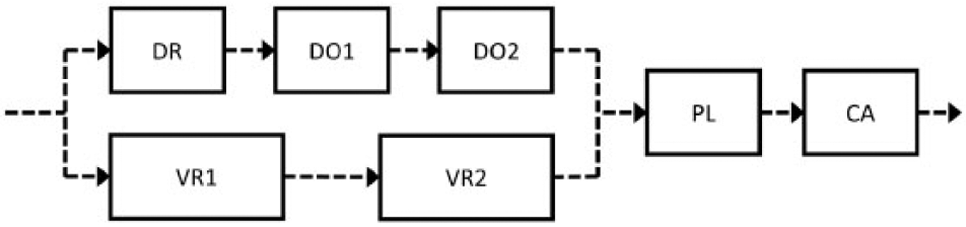
Upper respiratory tract model schematic. There are compartments representing the dorsal respiratory (DR), anterior dorsal olfactory (DO1), posterior dorsal olfactory (DO2), anterior ventral respiratory (VR1), posterior ventral respiratory (VR2), pharynx and larynx (PL), and conducting airways (CA) regions. The dashed line arrows represent air flows due to respiration. There are also blood flows to each of the seven subcompartments in the upper respiratory tract, but these are not shown here.

The model schematic in Figure 1 includes several features that were not present in the Campbell et al. (2014) model. We have added to that model a compartment representing the exposed portion of the SC and another representing the underlying VE, as well as a compartment representing an “exposure well.” (The two “application wells” in the study of Kim et al. [2006] were modeled as a single exposure well.) The volumes (ml) of the SC and VE were calculated using thickness (cm) and exposure surface area (cm²) parameters, and the volume of the VE was subtracted from total volume of the richly perfused tissue compartment proposed by Campbell et al. (2014). Also, the blood flow rate to the VE was computed by multiplying the volume proportion of the richly perfused tissue that is the VE by the Campbell et al. (2014) richly perfused tissue blood flow rate.

We implemented the skin components of the model (ie, the SC and VE compartments) and the exposure well using two approaches to create two distinct models, which we then compared in terms of their abilities to describe time-course blood concentration data from the Kim et al. (2006) study. Both models include an exposure well that contains naphthalene in a vehicle medium. For the dataset we considered (Kim et al., 2006), the vehicle was JP-8 and so many symbols in the discussion below involve the code “JP-8”; however, the models described here could be used in cases where the vehicle is something other than JP-8.

In the first skin modeling approach, hereafter referred to as the 2C approach, a basic 2C skin model (McCarley and Bunge, 2001) was used. The rate of change of the amount of naphthalene in the exposure well was assumed to be

$$\frac{d}{dt}{A}_{\text{well }}(t)=-P_{\text{SCJP}8}\cdot E\cdot \left(C_{\text{well }}(t)-\frac{C_{\text{SC }}(t)}{H_{\text{SC}:\text{JP}8}}\right),$$ (1)

where P_SCJP8 is the steady-state permeability (cm/min) of JP-8 through the SC, E is the surface area (cm²) of the SC that is exposed (at its interface with the exposure well), H_SC:JP8 is a partition coefficient representing the ratio of the equilibrium naphthalene concentrations in SC versus JP-8, and C_well(t) and C_SC(t) are the concentrations in the exposure well and in the SC compartment, respectively, at time t. We assumed these two concentrations to be spatially uniform at any given time within their respective compartments; ie, the exposure well and SC compartments are both assumed to be “well-mixed.” The steady-state permeability through the SC was computed as

$$P_{\text{SCJP}8}=\frac{H_{\text{SC}:\text{JP}8}\cdot D_{\text{SC }}}{T_{\text{SC }}},$$

where D_SC (cm²/min) is the effective diffusivity of naphthalene through the SC, and T_SC is the thickness (cm) of the SC (McCarley and Bunge, 2001). A “zero-flux” condition (eliminating movement of naphthalene between the exposure well and the SC) was enforced for times after the end of exposure (t_exp) by setting the time rate of change of A_well(t) to zero for t > t_exp.

In the 2C version of the model, the amount of naphthalene in the SC is given by

$$\frac{d}{dt}{A}_{\text{SC}}(t)=P_{\text{SCJP}8}\cdot E\cdot \left(C_{\text{well}}\left(t\right)-\frac{C_{\text{SC}}(t)}{H_{\text{SC}:\text{JP}8}}\right)+P_{\text{VEJP}8}\cdot E\cdot \left(\frac{C_{\text{VE}}\left(t\right)}{H_{\text{VE}:\text{JP}8}}-\frac{C_{\text{SC}}\left(t\right)}{H_{\text{SC}:\text{JP}8}}\right),$$ (2)

where P_VEJP8 is the steady-state permeability (cm/min) of JP-8 through the VE, H_VE:JP8 is a partition coefficient representing the ratio of the equilibrium naphthalene concentrations in VE versus JP-8, and C_VE(t) is the concentration in the VE at time t. In practice, we calculated the value of H_VE:JP8 as H_SC:JP8/H_SC:VE, where H_SC:VE is a partition coefficient representing the ratio of the equilibrium naphthalene concentrations in SC versus VE. The VE is assumed to be well-mixed. The steady-state permeability was computed as

$$P_{\text{VEJP8 }}=\frac{H_{\text{VE:JP}8}\cdot D_{\text{VE}}}{T_{\text{VE}}},$$

where D_VE (cm²/min) is the effective diffusivity of naphthalene through the VE, and T_VE is the thickness (cm) of the VE (McCarley and Bunge, 2001). The first term in Equation 2 was set to zero for t > t_exp to enforce the zero-flux condition previously described.

The amount of naphthalene in the VE is given by

$$\frac{d}{dt}{A}_{\text{VE}}\left(t\right)=-P_{\text{VEJP}8}\cdot E\cdot \left(\frac{C_{\text{VE}}(t)}{H_{\text{VE}:\text{JP}8}}-\frac{C_{\text{SC}}(t)}{H_{\text{SC}:\text{JP}8}}\right)+Q_{\text{VE}}\cdot \left(C_{\text{AB}}\left(t\right)-\frac{{\text{C}}_{\text{VE}}\left(t\right)}{H_{\text{VE}:\text{blood}}}\right),$$ (3)

where Q_VE is the blood flow rate (ml/min) into and out of the VE compartment (cf. Figure 1), C_AB(t) is the concentration (nmol/ml) in the arterial blood compartment, C_VE(t) is the concentration (nmol/ml) in the VE, H_VE:blood is the partition coefficient describing the ratio of the concentrations in VE and blood at equilibrium.

In the 2C version of the model, we added three new state variables to the Campbell et al. (2014) model: one representing the amount of naphthalene in the exposure well that is in contact with the SC (cf. Equation 1), one representing the amount of naphthalene in the exposed portion of the SC (cf. Equation 2), and one representing the amount of naphthalene in the exposed portion of the VE (cf. Equation 3). The ordinary differential equations (ODEs) for state variables representing amounts of naphthalene in compartments other than the exposure well, the SC, and the VE were identical to those used by Campbell et al. (2014) except that the state equation for the amount in the venous blood was altered to reflect flow into this compartment from the VE. We provide a complete listing of the model ODEs using the MCSim model specification language (Bois, 2009) in the Supplementary File “naph_pbtk_2c.model.” Tables 1–4 list the values we used for parameters that appear in the model equations.

Table 1.

General anatomical and physiological model parameters for humans

Parameter	Symbol	Value	Source
Body mass (g)	BWinit	70 000	a
Cardiorespiratory flow rates (ml/min/g0.75, to be multiplied by body mass to 0.75 power)
Cardiac output	QPUc	1.208	a, b, c
Minute ventilation	MVC	1.743	a, b, c
Tissue flow rates (proportion of cardiac output)
Liver	FBLI	0.23	a, b, c
Fat	FBFA	0.06	a, b, c
Poorly perfused	FBPP	0.2575	a, b
Richly perfused	FBRP	0.44	a, b, c
Upper respiratory tract	FBURT	0.0025	a, b, c
Conducting airways	FBCA	0.01	a
Tissue volumes (ml/g, to be multiplied by body mass)
Liver	FTLI	0.026	a, b, c
Fat	FFAT	0.136	a, b, c
Poorly perfused	FTPP	0.487	a, b, c
Richly perfused	FTRP	0.1861	a, b, c
Arterial blood	FTABD	0.022	a
Venous blood	FTVBD	0.045	a

^aCampbell et al. (2014), source code file “human.m.”

^bCampbell et al. (2014), Table 1, 2, or 3.

^cAdditional (original) sources are cited by Campbell et al. (2014).

Table 4.

Skin-related Parameters for Two-Compartment (2C) and Partial Differential Equation (PDE) Skin Models for Humans

Parameter	Symbols	Value	Source
Tissue dimensions
SC thickness (cm)	TSC, TSC	0.003	McCarley and Bunge (2001)
VE thickness (cm)	TVE, TVE	0.0075	McCarley and Bunge (2001)
Partition coefficients
SC:VE	HSC:VE, HSCVE	1.98	McCarley and Bunge (2001)
SC:JP-8	HSC:JP8, HSCJP8	Varies	Calibrated
VE:JP-8a	HVE:JP8, HVEJP8	Varies	Calculated
VE:blood	HVE:blood, HVEB	2.73	McCarley and Bunge (2001)
Diffusivity constants (cm2/min)
Naphthalene through SC	DSC, DSC	Varies	Calibrated
Naphthalene through VEa	DVE, DVE	0.00482	McCarley and Bunge (2001)
Exposure parameters
Intravenous dose rate (nmol/min)b	RIV	Varies	Calibrated
Surface area of exposed skin (cm2)	E, AEXP	20	Kim et al. (2006)
JP-8 volume in exposure well (ml)	VWELL	1.0	Kim et al. (2006)
Exposure time (min)	texp, exp_time	Varies	Kim et al. (2006)
Naphthalene conc. in JP-8 (g/ml)	CNJP8	0.003	Kim et al. (2006)

^aThese parameters were used in the 2C model but not in the PDE model.

^bIntravenous dose rate is used to account for “background” blood concentrations of naphthalene observed in the subjects from the Kim et al. (2006) study prior to exposure.

In the second skin modeling approach, hereafter referred to as the PDE approach, the concentration in the SC was modeled by directly applying Fick’s Second Law. This is similar to the approach of Kim et al. (2008), except that we did not assume that the overall thickness of the SC was decreased (due to removal of layers of skin) over the course of a skin exposure and tape stripping experiment. Thus, the concentration φ(x, t) (nmol/ml) at depth x (cm) and at time t (min) is given by

$$\frac{\partial }{\partial t}\phi \left(x,t\right)=D_{\text{SC}}\frac{{\partial }^2}{\partial x^2}\phi \left(x,t\right),$$ (4)

where D_SC (cm²/min) is the effective diffusivity of naphthalene through the SC. As for the 2C model, we assumed the concentrations in the exposure well, C_well(t), and the VE, C_VE(t), to be spatially uniform at any given time within their respective compartments. To obtain solutions to Equation 4 for values of x between 0 (which represents the outer surface of the SC and its interface with the exposure well) and T_SC (which represents the maximum depth of the SC and its interface with the VE) at times after some initial time t₀, two boundary conditions and one initial condition are required. We assumed boundary conditions given by

$$\phi \left(0,t\right)=H_{\text{SC:JP}8}{C}_{\text{well}}\left(t\right)$$ (5)

and

$$\phi \left(T_{\text{SC}},t\right)=H_{\text{SC:VE}}{C}_{\text{VE}}\left(t\right),$$ (6)

where H_SC:JP8 and H_SC:VE are partition coefficients previously defined for the 2C model. These two boundary conditions reflect instantaneous equilibrium between the SC and JP-8 at the outer surface of the SC and between the SC and the VE at the interface of those two skin compartments. We used an initial condition given by

$$\phi \left(x,t_0\right)=0$$ (7)

for all x between 0 and T_SC, reflecting an assumption that the SC contained no naphthalene at the start of skin exposure simulations.

To numerically solve the initial-and-boundary-value problem given by Equations 4 through 7, we discretized the spatial (depth) variable x by creating a uniform mesh with 11 nodes; ie, x_j = T_SC · j/10 for j in {0, 1, …, 10}. Then, we used central finite differences to approximate the second-order spatial derivatives in Equation 4 so that

$$\frac{d}{dt}{\phi }_j(t)=D_{\text{SC}}\cdot \frac{{\phi }_{j-1}(t)-2{\phi }_j(t)+{\phi }_{j+1}(t)}{{\left(T_{\text{SC}}/10\right)}^2}$$ (8)

for j in {1, 2, …, 9}, where φ_j(t) ≈ φ(x_j, t) and φ₀(t) and φ₁₀(t) are given by the boundary conditions in Equations 5 and 6, respectively.

In the PDE version of the model, the amount of naphthalene in the exposure well contacting the SC is given by

$$\frac{d}{dt}{A}_{\text{well }}\left(t\right)=-J\left(0,t\right)\cdot E,$$ (9)

where E is the surface area (cm²) of the SC that is exposed (at its interface with the exposure well) and

$$J(x,t)=-D_{\text{SC}}\cdot \frac{\partial }{\partial x}\phi \left(x,t\right)$$

is the naphthalene flux (nmol/cm²/min) at a depth x cm into the SC. (At the interface of the exposure well and the SC, x = 0.) We used a forward finite difference to compute the value of J₀(t) ≈ J(0, t) as

$$J_0\left(t\right)=-D_{\text{SC}}\cdot \frac{{\phi }_1(t)-{\phi }_0(t)}{\left(T_{\text{SC}}/10\right)}.$$

Thus, the approximation for Equation 9 becomes

$$\frac{d}{dt}{A}_{\text{well}}\left(t\right)=-D_{\text{SC}}\cdot \frac{{\phi }_1(t)-{\phi }_0(t)}{\left(T_{\text{SC}}/10\right)}\cdot E.$$ (10)

A zero-flux boundary condition (that replaces the boundary condition of Equation 5) was enforced for times after the end of exposure (t_exp) by setting φ₀(t) = φ₁(t) for t > t_exp.

The amount of naphthalene in the VE is given by

$$\frac{d}{dt}{A}_{\text{VE}}(t)=J\left(T_{\text{SC}},t\right)\cdot E+Q_{\text{VE}}\cdot \left(C_{\text{AB}}(t)-\frac{C_{\text{VE}}(t)}{H_{\text{VE:blood}}}\right),$$ (11)

where Q_VE, C_AB(t), C_VE(t), and H_VE:blood are parameters previously defined for Equation 3. We used a backward finite difference to compute the value of J₁₀(t) ≈ J(T_SC, t) as

$$J_{10}\left(t\right)=-D_{\text{SC}}\cdot \frac{{\phi }_{10}(t)-{\phi }_9(t)}{\left(T_{\text{SC}}/10\right)}.$$

Thus, the approximation for Equation 11 becomes

$$\frac{d}{dt}{A}_{\text{VE}}\left(t\right)=-D_{\text{SC}}\cdot \frac{{\phi }_{10}(t)-{\phi }_9(t)}{(L/10)}\cdot E+Q_{\text{VE}}\left(t\right)\cdot \left(C_{\text{AB}}(t)-\frac{C_{\text{VE}}(t)}{H_{\text{VE:blood}}}\right).$$ (12)

In the PDE version of the model, 11 new state variables were added to the Campbell et al. (2014) model: one representing the amount of naphthalene in the exposure well that is contact with the SC (cf. Equation 10), nine representing concentrations of naphthalene at the interior nodes of the exposed portion of the SC (cf. Equation 8 for j in {1, 2, …, 9}), and one representing the amount of naphthalene in the exposed portion of the VE (cf. Equation 12). We provide a complete listing of the model ODEs for the PDE version of the model using the MCSim model specification language (Bois, 2009) in the Supplementary File “naph_pbtk_pde.model.” Tables 1–4 list the values we used for parameters that appear in the model equations.

Model Calibration

We estimated values for three parameters common to the two PBPK models (ie, the 2C and the PDE) by calibrating the models to the Kim et al. (2006) data. The calibration parameters were: DSC, the effective diffusivity of naphthalene through the SC (cm²/min); HSCJP8, the SC-to-JP-8 partition coefficient; RIV, the rate of intravenous dosing (nmol/min). The human data revealed measurable blood concentrations of naphthalene present in the subjects prior to skin exposure, so we used the intravenous dose-rate parameter RIV to account for these baseline blood levels. We performed the calibration by finding sets of values for these three parameters for each subject that minimized the sum of squared errors (SSE), where “errors” are differences between the observed concentrations of naphthalene in blood and those blood concentrations predicted by the model for the specified set of parameter values; ie, we estimated the parameters using the ordinary least squares method. The model-predicted concentrations were obtained by performing model simulations based on the experimental conditions and features of the subjects from the Kim et al. (2006) study. In particular, in addition to varying the values of DSC, HSCJP8, and RIV, we used recorded study data to specify values for model parameters such as the subject body mass (BWinit), the surface area of the exposed skin (AEXP), and the duration of exposure (exp_time) (cf. Tables 1 and 4).

For both models, we used the R function “optim” to find the values of DSC, HSCJP8, and RIV that minimize the SSE for subject-specific data. Thus, in each case (for the 2C and the PDE models) we obtained ten sets of parameter values for ten subjects. Implementations for these calibrations can be found in the Supplementary Files “skin_exp_2c_fit_indiv.R” and “skin_exp_pde_fit_indiv2.R.” For the PDE model, we also found a set of 21 parameters that minimizes the total SSE for all subjects simultaneously. For this calibration, DSC and RIV were allowed to take on different values for each subject (for a total of 20 parameter values), but the value of HSCJP8 was assumed to be the same for all subjects (adding one more parameter value). The implementation for this calibration can be found in the Supplementary File “skin_exp_pde_fit_all.R.”

Sensitivity Analysis

To assess the sensitivity of the PDE model, we computed local sensitivity indices for all parameters. For this analysis, we conducted model simulations of a skin exposure scenario based on the conditions of the Kim et al. (2006) study and examined four dose metrics (ie, model outputs): (1) the average blood concentration during the 24-h period starting with the beginning of the skin exposure; (2) the difference between this average blood concentration and the steady-state blood concentration prior to the beginning of skin exposure (which arises due to an intravenous dose); (3) the peak arterial blood concentration during the 24-h period; and (4) the difference between this peak blood concentration and the steady-state blood concentration. The normalized local sensitivity index for each parameter for a given dose metric was computed as

$$S_i=\frac{f\left(\widehat{q}+h_i\cdot {\overrightarrow{e}}_i\right)-f\left(\widehat{q}\right)}{h_i}\cdot \frac{{\widehat{q}}_i}{f\left(\widehat{q}\right)},$$ (13)

where $\widehat{q}$ is a vector containing a “local” set of values for all model parameters, $f\left(\overrightarrow{q}\right)$ is the value of the dose metric for the parameter values in a vector $\overrightarrow{q}$, ${\overrightarrow{e}}_i$ is the ith standard basis vector (with a 1 in the ith position and zeros elsewhere), ${\widehat{q}}_i$ is the local value of the the ith parameter (ie, the ith component of the vector $\widehat{q}$), and h_i is a “small” perturbation to the ith parameter. We computed the small perturbation as

$$h_i=\{\begin{array}{cc}\hfill ϵ\cdot {\widehat{q}}_i\hfill & \text{if}{\widehat{q}}_i\ge ϵ/\left(1+ϵ\right),\hfill \\ \hfill ϵ-{\widehat{q}}_i\hfill & \text{if}{\widehat{q}}_i<ϵ/\left(1+ϵ\right)\text{and}{\widehat{q}}_i\ge 0,\hfill \\ \hfill -ϵ-{\widehat{q}}_i\hfill & \text{if}{\widehat{q}}_i<ϵ/\left(1+ϵ\right)\text{and}{\widehat{q}}_i<0,\hfill \end{array}$$

where ϵ = 10⁻².

The normalized local sensitivity index represents the ratio of the relative change in the dose metric to the relative change in a single parameter. We computed one sensitivity index per dose metric for each model parameter based on the local set of parameter values provided in Tables 1–4. The local parameter values used for DSC, HSCJP8, and RIV were based on average values obtained by model calibration for the ten subjects from the Kim et al. (2006) study. The duration of exposure (exp_time) was taken to be 36 min, which is the mode of the exposure times recorded for the Kim et al. (2006) subjects. The sensitivity analysis algorithm can be found in the Supplementary File “sensitivity_analysis.R.”

SC Concentration Profiles

The PDE model can be used to generate concentration versus depth profiles for the SC. To illustrate this capability, we conducted a model simulation of a skin exposure scenario based on the conditions of the Kim et al. (2006) study and generated concentration profiles at various times between 0.1 and 5 h after the start of exposure. The local parameter values used for DSC, HSCJP8, and RIV were based on average values obtained by model calibration for the ten subjects from the Kim et al. (2006) study and the duration of exposure (exp_time) was taken to be 36 min (as was done for the sensitivity analysis). The Supplementary File“skin_concentration_profile.R” contains a script that performs the simulation and generates plots showing the concentration profiles.

Comparison of Skin and “Background” Exposures

To compare the relative amounts of naphthalene delivered via the controlled skin exposure of Kim et al. (2006) and the “background” exposure (which we accounted for using a continuous intravenous dose), we simulated 10⁵ min (about 70 days) of intravenous dosing (to allow for blood concentrations to reach steady-state) followed by 36 min of skin exposure (which was the mode of the exposure durations for the Kim et al. [2006] subjects). We continued the simulation up until 5 h after the beginning the skin exposure and maintained the intravenous dosing rate for the entire simulation. We then computed the total amount of naphthalene absorbed from the exposure well and the total amount administered intravenously during the 5 h following the beginning of the skin exposure. The method described here is implemented in the Supplementary File “comp_skin_to_iv_exp.R.”

Evaluation of Model Numerical Precision

To numerically solve the ODEs that define the models, we used the default ODE integrator (ie, the function “ode”) of the R package “deSolve” and specified absolute and relative error tolerances of 10⁻⁶; however, in the case of the PDE model, the precision of the integration method was further limited by the method we used to discretize the PDE. Recall that we discretized the spatial variable x (which represents position or depth the SC) using 11 nodes. If the number of nodes is N + 1, the error in the PDE discretization method (central finite differences) is O(1/N²), the error in the method used to calculate the amount in the SC (trapezoid rule) is also O(1/N²), and the error in the method used to calculate the flux out of the exposure well (forward finite difference) is O(1/N). To estimate precision of the model with respect to mass balance, we computed the total mass of naphthalene that has entered the organism (at any given simulation time) in two different ways: (1) by calculating the net mass of naphthalene that has moved into the organism via inhalation, exhalation, intravenous injection, and flux out of the exposure well [which has O(1/N) error]; and (2) by calculating the total amount in the organism, including the amount in the SC [which has O(1/N²) error], plus the cumulative amount that has been metabolized. The method described here is implemented in the Supplementary File “numerical_analysis.R.”

Quality Assurance

We applied a quality assurance protocol (U.S. EPA, 2018) to ensure that the PBPK models we developed meet various quality standards. In particular, we verified that the model implementation software, which is available in the Supplementary Material, agrees with the model description outlined in this manuscript and the model parameter values match values from the cited sources.

RESULTS

Model Calibration

We calibrated the PDE and SC models to the Kim et al. (2006) data to obtain optimal values for the parameters RIV, DSC, and HSCJP8. Figure 3 shows the Kim et al. (2006)time-course blood concentration data for ten subjects along with the calibrated model predictions for the PDE model (which was calibrated in two different ways) and the 2C model. Note that the increase in naphthalene blood concentration following the skin exposure was markedly higher for Subject 1 than for any other subject.

Figure 3.

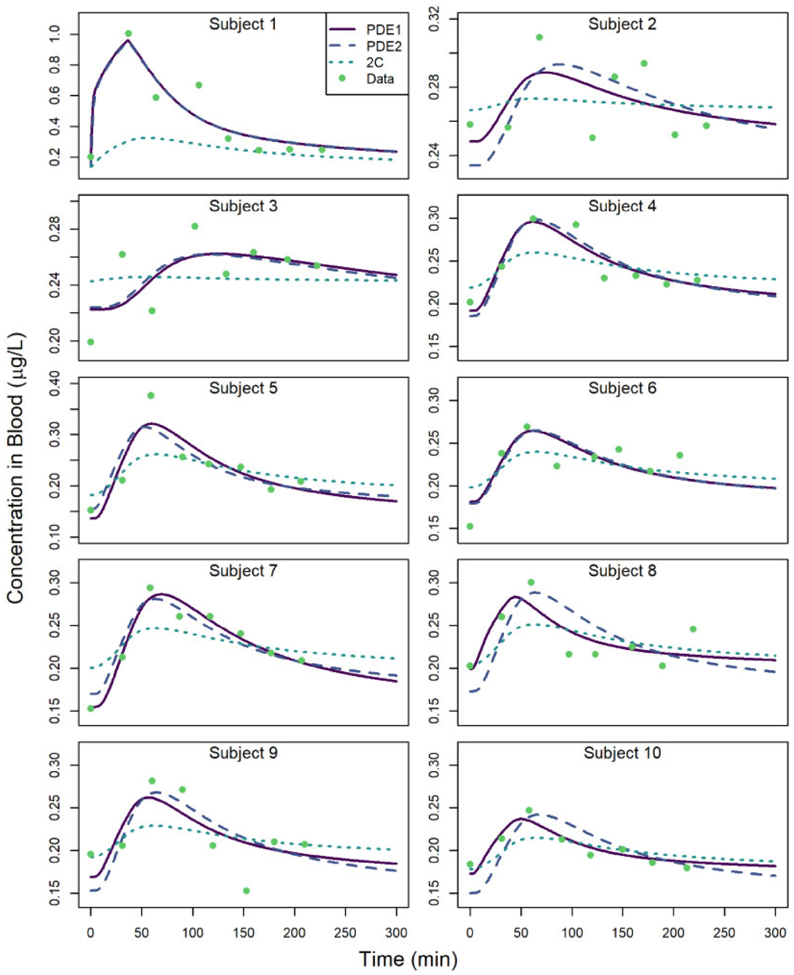
Naphthalene blood concentrations versus time for subjects from the study of Kim et al. (2006). Observed data are depicted along with model-predicted values when calibrating the partial differential equation (PDE) model to individual subject data (“PDE1”), when calibrating the PDE model to all subjects simultaneously assuming a constant HSCJP8 (“PDE2”), and when calibrating the two-compartment (2C) model to individual subject data (“2C”).

Table 5 shows the optimal parameter values for the PDE model that were obtained by calibrating to the individual subject data independently, whereas Table 6 shows the parameter values that were obtained by calibrating to the subject data simultaneously under the assumption that HSCJP8 is identical for all subjects. The optimal parameter values obtained for the 2C model are shown in the Supplementary File “supplemental_2C_params.docx.” In both Tables 5 and 6, two sets of values are provided for the mean and coefficient of variation (CV) for each of the three parameters. In each case, the first mean and CV reflect parameter values obtained for all ten subjects and the second mean and CV are based only on Subjects 2 through 10. We omitted the parameter values for Subject 1 in the calculations for the second set of numbers because the time-course concentration data, and consequently the estimated value of DSC, for that subject were very different from those of the other subjects (cf. Figure 3); we therefore wanted to conduct an alternate analysis based on the hypothesis that this subject may have been different from the other subjects in some way.

Table 5.

Values for the Parameters RIV, DSC, and HSCJP8 in the Partial Differential Equation Model When Calibrating the Model to Time-course Blood Concentration Data for Each Subject Independently

Subject	RIV (nmol/min)	DSC (cm2/min)	HSCJP8
1	1.34	2.34 × 10−5	0.201
2	1.69	6.96 × 10−8	0.0942
3	1.44	2.64 × 10−8	0.250
4	1.32	1.04 × 10−7	0.167
5	1.14	1.18 × 10−7	0.330
6	1.70	1.09 × 10−7	0.182
7	1.16	8.04 × 10−8	0.301
8	1.42	3.38 × 10−7	0.0506
9	1.13	1.26 × 10−7	0.122
10	1.41	2.31 × 10−7	0.0596
Mean	1.38	2.46 × 10−6	0.176
CV (%)	14.8	299.1	55.2
Meana	1.38	1.34 × 10−7	0.173
CVa (%)	15.7	70.7	59.2

^aThe mean and coefficient of variation (CV) values shown in the last two rows are computed using values obtained for Subjects 2 through 9; ie, Subject 1 values are omitted from the calculations.

Table 6.

Values for the Parameters RIV, DSC, and HSCJP8 in the Partial Differential Equation Model When Calibrating the Model to Time-course Blood Concentration Data for All Subjects Simultaneously and Assuming HSCJP8 Has the Same Value for All Subjects

Subject	RIV (nmol/min)	DSC (cm2/min)	HSCJP8
1	1.38	1.19 × 10−5	0.204
2	1.59	4.80 × 10−8	0.204
3	1.46	3.02 × 10−8	0.204
4	1.28	9.15 × 10−8	0.204
5	1.29	1.72 × 10−7	0.204
6	1.68	9.94 × 10−8	0.204
7	1.78	1.01 × 10−7	0.204
8	1.23	9.76 × 10−8	0.204
9	1.02	9.10 × 10−8	0.204
10	1.23	8.76 × 10−8	0.204
Mean	1.34	1.27 × 10−6	0.204
CV (%)	14.2	293.6	N/A
Meana	1.34	9.09 × 10−8	0.204
CVa (%)	15.1	43.2	N/A

^aThe mean and coefficient of variation (CV) values shown in the last two rows are computed using values obtained for Subjects 2 through 9; ie, Subject 1 values are omitted from the calculations.

Abbreviation: N/A, not applicable.

Figure 3 reveals that the PDE model generally provides a better fit to the data than the 2C model. However, as shown in Table 5, a wide range of parameter values are required to ensure model agreement with data for all subjects. For example, the CV for the DSC parameter is nearly 300% when considering all ten subjects and is still greater than 70% when omitting Subject 1 (for whom the changes in blood concentration levels were considerably greater) from consideration. These large CVs may arise because of interactions between model parameters that limit one’s ability to uniquely identify all three of the calibration parameters. To address this issue, we calibrated the PDE model in a second way. We hypothesized that HSCJP8 (the SC-to-JP-8 partition coefficient) should be relatively consistent for all subjects, but that RIV (which reflects the subject’s background exposure to naphthalene) and DSC (which is, nominally, the diffusivity of naphthalene through the subject’s SC, but which may also reflect differences in the depth and spacing of hair follicles and the overall thickness of the SC) could vary considerably between subjects. In the second calibration scheme, we therefore selected a set of optimal parameters by calibrating to all subject data simultaneously and assuming HSCJP8 has the same value for all subjects. The results of this second calibration are shown in Table 6 and Figure 3. For this calibration, the CV for the DSC parameter is greatly reduced (43% when omitting Subject 1), whereas the CV for the RIV parameter is about the same (approximately 15%) for both calibrations. In this second calibration, HSCJP8 does not vary at all (by design), whereas in the first calibration this parameter had a CV of nearly 60% (whether Subject 1 was omitted or not). Thus, overall variability in the optimal parameter values for the ten subjects was greatly reduced when assuming that HSCJP8 has the same value for all subjects. Also, as shown in Figure 3, the overall agreement of the PDE model and the data is not greatly impacted when calibrating the parameters under this assumption.

For the calibrated PDE model, the maximum percent difference between model predicted concentrations and observed concentrations in blood was 37.8%, and the average percent difference was 8.94%. To evaluate predictions of the part of the blood concentration attributable to the controlled skin exposure, we subtracted the first predicted concentration for each subject (which represents the baseline concentration) from both the predictions and the observations and then computed percent errors in the adjusted predictions based on the adjusted observations. Using this metric, most (96.25%) of the predictions of the increase in blood concentrations due to skin exposure were within a factor of 2 of the observations. The median absolute percent error was 27.1%.

Sensitivity Analysis

Figure 4 shows the relative sizes of the normalized sensitivity indices for four dose metrics: (1) the average blood concentration during the 24-h period starting with the beginning of the skin exposure; (2) the difference between this average blood concentration and the steady-state blood concentration prior to the beginning of skin exposure (which arises due to an intravenous dose); (3) the peak arterial blood concentration during the 24-h period; and (4) the difference between this peak blood concentration and the steady-state blood concentration. In this figure, we have only included those parameters for which at least one of the four sensitivity indices had an absolute value greater than 0.2. The values of the sensitivity indices for all parameters and all four dose metrics can be found in the Supplementary File “sensitivity.csv.”

Figure 4.

Normalized sensitivity indices (cf. Equation 13) for dose metric 1 (average blood concentration following skin exposure), dose metric 2 (difference between average blood concentration and steady-state blood concentration), dose metric 3 (peak blood concentration following skin exposure), and dose metric 4 (difference between peak blood concentration and steady-state blood concentration).

Dose metrics 1 and 3 assess the degree to which internal dose (average and peak blood concentration) is impacted overall by both the intravenous and the skin exposure, whereas dose metrics 2 and 4 assess the degree to which internal dose is impacted by the skin exposure alone (because the “baseline” steady-state blood concentration is subtracted from these metrics). Thus, we see in Figure 4 that RIV (the intravenous dose rate parameter) has a relatively large impact on dose metrics 1 and 3 but hardly any impact on dose metrics 2 and 4. Similarly, the parameters that we expect to impact the skin dose (CNJP8, HSCJP8, AEXP, and exp_time) all have relatively large impacts on dose metrics 2 and 4, and considerably smaller impacts on dose metrics 1 and 3 (where RIV has more influence). We remark that CNJP8 (the concentration of naphthalene in the JP-8 applied to the skin), HSCJP8 (the SC-to-JP-8 partition coefficient), and AEXP (the surface area of the exposed skin) all have sensitivity indices of approximately 1 for dose metrics 2 and 4; this implies that a 1% increase in any of those parameters would lead to a 1% increase in either dose metric. The parameter exp_time (which represents the duration of skin exposure) has also a positive and substantial sensitivity index for both dose metrics 2 and 4, but the value is in both cases considerably less than 1. Thus, exp_time is less influential than the other parameters that define the skin exposure period.

Body mass (BWinit) has a negative impact on all the internal dose metrics because, for the fixed concentration applied to the skin, a larger person will generally have a larger volume of distribution and therefore the blood concentrations that arise in the person will be smaller. The fraction of cardiac output that flows to the liver (FBLI) has a negative impact because more blood flow to the liver corresponds to higher metabolic capacity. Similarly, the cardiac output parameter (QPUc), itself, has a negative impact because greater overall blood flow through the body corresponds to more clearance via metabolism and air exchange. None of the dose metrics are sensitive to the metabolic capacity of the liver (VmaxLI), suggesting that clearance is limited by blood flow for the exposure scenario considered.

SC Concentration Profiles

Figure 5 shows concentration versus depth profiles for the SC at 11 time points following the start of a 36-min exposure. The concentration at the outer surface of the SC (at depth 0 μm) prior to 36 min, when the JP-8 was still in contact with the skin, remained relatively constant (as shown in the profile curves representing times from 0.1 to 0.6 h after the start of exposure) and decreased thereafter (as shown in the profile curves representing times after the removal of the JP-8 at 0.6 h). The concentration at the interface of the SC and the VE (at depth 3 μm) was relatively low shortly at 0.1 h after the start of exposure but increased substantially by 0.6 h (when the JP-8 was removed from the skin surface). The concentration at that interface continued to increase after the JP-8 was removed as evidenced by the profile curves representing 0.7–1 h after the start of exposure, but by 2 h had decreased to a concentration less than the 0.6 h concentration. By 5 h after the start of exposure (4.4 h after the removal of the JP-8 from the skin surface), the concentration across the SC was approximately zero.

Figure 5.

Naphthalene concentrations in stratum corneum (SC) versus SC depth at various times between 0.1 and 5 h following the start of a 36-min (0.6-h) skin exposure.

Comparison of Skin and “Background” Exposures

We performed a simulation (described in the Materials and Methods section) to compare the relative amounts of naphthalene delivered via the controlled skin exposure of Kim et al. (2006) and the background exposure (which we modeled as a constant, continuous intravenous dose). The total amount absorbed from the exposure well into the SC during the simulated 5-h period was 23.4 μg, whereas the total amount delivered intravenously during that time was 51.5 μg. That is, background exposure was apparently responsible for the delivery of more than 2 times more naphthalene than was the controlled skin exposure.

Numerical Precision of PDE Model

We found that using 11 nodes (N = 10) to discretize the PDE model gave reasonable model precision based on mass balance. To estimate this precision, we computed the total mass of naphthalene that has entered the organism in two different ways: (1) by calculating the net mass of naphthalene that has moved into the organism; and (2) by calculating the total amount in the organism plus the cumulative amount that has been metabolized. The maximum relative discrepancy in the total amount of naphthalene (as calculated using these two approaches) was 0.0115%. At the time of this maximum, the discrepancy was 0.00195 mg and the total amount of naphthalene (which we estimated as the average of the values calculated using the two approaches) was 16.999 mg.

DISCUSSION

PBPK models provide a means for predicting internal dose metrics, such as tissue concentrations and rates of metabolism, that arise from external ones, such as administered oral doses or inhaled air concentrations (IPCS, 2010; U.S. EPA, 2006). The ability to translate between internal and external doses proves valuable in characterizing dose-response relationships and health risks because biological responses are believed to be more directly related to measures of internally delivered dose than to external doses or exposures (IPCS, 2010; U.S. EPA, 2006). One can parameterize PBPK models via in vitro-to-in vivo extrapolation (IVIVE) (see eg, the chloroprene model of Yang et al. [2012]), and Campbell et al. (2014) used IVIVE-informed values for several metabolic parameters in their naphthalene PBPK model; however, assumptions and calculations inherent in IVIVE lead to increased quantitative uncertainty in model predictions. Successful comparison of IVIVE model predictions to even limited in vivo PK data can help offset this additional uncertainty. In this study, we sought to evaluate the Campbell et al. (2014) PBPK model for naphthalene for potential use in human health risk assessment. That model has been used for nasal tissue dosimetry (which is relevant to the nasal toxicity observed in rodents) and those authors evaluated the model using in vivo rodent PK data but not in vivo human PK data. We identified a human PK dataset based on a controlled skin exposure study (Kim et al., 2006) and expanded the Campbell et al. (2014) model so that such a study could be simulated. Predictions generated with our augmented PBPK model showed reasonable agreement with in vivo human blood concentration data: by adjusting only those parameters that determine background exposure and skin transport, the increase in blood concentration due to the controlled skin exposures was replicated to within a factor of 2 for the majority of the Kim et al. (2006) observations.

2C Versus PDE Skin Models

In augmenting the Campbell et al. (2014) model to accommodate skin exposure, we considered both 2C and PDE representations of the skin. In the 2C model, the SC and the VE were each represented by a single compartment. In the PDE model, the VE was represented by a single compartment but the SC was represented by a PDE that was spatially discretized. The 2C and the PDE models were calibrated using the same three parameters, but the PDE model gave a better overall fit to the time-course blood concentration data from the Kim et al. (2006) study (cf. Figure 3). The better fit of the PDE model likely arises because it effectively includes more “compartments” in its representation of the SC, which allows for faster initial absorption followed by slower release of naphthalene into the VE and then into systemic circulation.

Comparison of Values for Skin Exposure Parameters

Diffusivity quantifies the rate at which a substance can diffuse into a medium. By calibrating our PDE model to data from the Kim et al. (2006) subjects, we obtained average values of 1.27 × 10⁻⁶ and 9.09 × 10⁻⁸ cm²/min (the latter when omitting Subject 1) for the diffusivity of naphthalene across the SC (cf. Table 6). The second value is comparable with the value of 4.2 × 10⁻⁸ cm²/min obtained by Kim et al. (2008). The difference may, in part, be attributed to the fact that Kim et al. (2008) assumed a thickness of 0.002 cm for the SC, whereas we assumed the thickness to be 0.003 cm. The diffusivity value 1 obtains using the empirical formula (Equation 28) of McCarley and Bunge (2001) with an SC thickness of 0.003 cm and a naphthalene molecular weight of 128.17 g/mol is 1.4 × 10⁻⁶ cm²/min, which is more comparable with the first value we obtained, but which differs by about 1.0–1.5 orders of magnitude from the other values given above.

Notably, the blood concentration levels (which we used for calibration) are not particularly sensitive to the SC diffusivity parameter (DSC). (Sensitivity indices for this parameter were not presented in Figure 4, but values of these indices for DSC for the dose metrics we considered had values ranging from 4.6 × 10⁻⁶ to 9.3 × 10⁻⁵.) The lack of sensitivity of the difference-from-steady-state concentrations (ie, dose metrics 2 and 4) to diffusivity is somewhat surprising because the diffusivity should to some extent control the rate of exposure. Based on the calculated sensitivity indices, however, difference-from-steady-state concentrations are much more sensitive to the SC-to-JP-8 partition coefficient (HSCJP8), which controls the rate of absorption of naphthalene into the SC from the exposure well containing JP-8. The fraction of cardiac output that flows to the richly perfused tissue (FBRP), upon which blood flow to the VE depends, also exerts considerable influence on the difference between peak concentration and steady-state concentration (dose metric 4). Because diffusivity (DSC) has relatively little influence on the blood concentration levels, we do not expect our estimates of the value of this parameter to be very accurate.

Despite the relatively small influence of the parameter DSC reflected in the parameter sensitivity indices, we were able to account for the large differences in blood concentrations of Subject 1 relative to the other subjects of Kim et al. (2006) (cf. Figure 3) by using a relatively large value of DSC in the model simulations for Subject 1 (cf. Table 6). Thus, it seems plausible that Subject 1 had skin qualities pertinent to diffusivity (eg, fat content of or density of follicles on the skin) that differed substantially from those of the other subjects.

Uncertainty and Variability for Skin Exposure Parameters

Kim et al. (2007) obtained most physiological parameters, partition coefficients, and metabolism parameters for their naphthalene skin penetration model from the literature (Abraham et al., 1985; Brown et al., 1997; Fiserova-Bergerova et al., 1984; Hansch et al., 1995; Willems et al., 2001), but they estimated values for parameters describing SC uptake, VE permeability, fat-to-blood partitioning, and other-tissue-to-blood partitioning by calibrating their model to the blood time-course data of Kim et al. (2006). For these four calibrated parameters, Kim et al. (2007) reported values corresponding to CVs of 180%, 70%, 208%, and 112%, respectively. This variability in parameter values is comparable with that observed by us (cf. Table 5) when calibrating our PDE model to blood concentration data for each subject independently; however, (1) we only calibrated three parameters (whereas Kim et al. [2007] calibrated four) and (2) we were able to greatly reduce the variability in the parameter estimates when constraining the SC-to-JP-8 partition coefficient to have the same value for all subjects (cf. Table 6). Furthermore, we observe that Kim et al. (2007) adjusted the data of Kim et al. (2006) by subtracting baseline blood concentration levels before performing their calibrations, whereas we used the unadjusted data for our calibrations. Given that we were able to obtain reasonable agreement between model predictions and data using a model with only three calibrated parameters (one of which was essentially “fixed” for all subjects and another of which accounted for baseline blood concentrations) we contend that the Kim et al. (2007) model was likely overspecified in the sense that it included more parameters than can be uniquely identified using the Kim et al. (2006) data.

Partition coefficients, such as the SC-to-JP-8 partition coefficient HSCJP8, do not generally show high interindividual, or even interspecies, variation; however, DSC, which represents the diffusivity of naphthalene through a subject’s SC but which may also reflect other skin features, such as the overall thickness of the SC, could vary considerably between subjects. Kim et al. (2006) only collected data for ten subjects, but our results (cf. Table 6) provide some indication of interindividual variability in DSC for these subjects. For comparison, note that van de Sandt et al. (2004) evaluated skin absorption of caffeine, testosterone, and benzoic acid across multiple laboratories by in vitro methods using skin from five to seven donors per substance. Although other sources of variability were evaluated, a primary conclusion of the analysis was that “the variation observed may be largely attributed to human variability in dermal absorption and the skin source,” with a CV (for skin absorption) ranging from 63% for caffeine to 120% for testosterone (van de Sandt et al., 2004). Variation in absorption depends on differences in both the partition coefficient and diffusivity, and whereas the results of van de Sandt et al. (2004) cannot be used to apportion total variation in absorption to these two parameters, neither of these are parameters that might be expected to vary significantly between individuals for other tissues (eg, liver). Nonetheless, the findings of van de Sandt et al. (2004) support our assumption that the primary source of variability in the time-course blood data of Kim et al. (2006) is variation in skin absorption. In any case, naturally occurring human variation in SC diffusivity, as well as variation in metabolic parameters and other anatomical and biochemical parameters in our PBPK model, should be considered when applying the model for risk assessment purposes.

Frasch et al. (2007) found that chemical penetration of skin can, in general, differ when the skin is exposed to a pure (“neat”) chemical versus an aqueous vehicle containing the chemical. Prolonged exposure to a solvent (ie, an aqueous vehicle) may cause the skin to swell as it becomes infused with the solvent and has the potential to change both the partitioning between the skin and the solvent and the diffusivity of the compound of interest (eg, naphthalene) through the skin. Thus, the SC-to-vehicle partition coefficient (HSCJP8) and diffusivity (DSC) parameters in our model may both be different for different vehicles. For this reason, the values of HSCJP8 and DSC estimated in our model calibrations using the Kim et al. (2006) dataset might not apply when using our model to simulate naphthalene skin exposures involving vehicles other than JP-8. The relatively high sensitivity indices we calculated for the vehicle-specific model parameter HSCJP8 (cf. Figure 4) suggest that it may be particularly important to adjust this parameter when considering other vehicles. One could use an experimental method to determine an appropriate value of the SC-to-vehicle partition coefficient for another vehicle or perform model calibrations such as those we have described but using a dataset that involves skin exposures with the vehicle of interest.

Baseline Blood Concentrations and Background Exposures

The data of Kim et al. (2006) reveal baseline blood concentrations of naphthalene present in all the subjects prior to skin exposure, so we used a constant intravenous dose rate parameter (representing the net rate at which naphthalene is delivered to the blood due to environmental exposure) to account for these. The baseline levels of naphthalene observed in the Kim et al. (2006) subjects are likely due to environmental exposures; however, the background exposures apparently experienced by these subjects exceed estimates of typical naphthalene exposures for adults in the U.S. population. For example, the subjects apparently experienced (prior to the controlled skin exposures) approximately 10 times the intake rate estimated (by us) from CDC (2019) urine metabolite data for U.S. smokers and more than 2 times the total daily naphthalene intake estimate of U.S. EPA (2003). A more detailed explanation of these comparisons, as well as comparisons between the estimated background exposures and U.S. EPA (1998) toxicity reference values, is provided in the Supplementary File “baseline_blood_concentrations.docx.” Higher background exposures can occur inside cars commuting in traffic, in freshly painted interiors of buildings, and in some urban locations (Preuss et al., 2003). If the study participants spent time in 1 or more of these environments prior to the experiments, this could account for the high levels of naphthalene observed in their blood.

The background exposure rate parameter RIV allows for model simulations of scenarios in which naphthalene is introduced to an organism through means other than known inhalation or skin exposures. In any given application of the model, one can assign a high or a low value to RIV (or even a value of zero for a scenario with no background exposure) as suggested by study data or other considerations. For risk assessment applications, one might wish to consider a variety of background exposure levels. For example, when evaluating the impact of naphthalene concentration in air on internal dose metrics (such as naphthalene concentration or rate of production of naphthalene metabolites in respiratory tissues), one could simulate individuals with both lower and higher background exposure rates to determine how background exposure affects the relationship between inhalation exposure and internal dose.

Experimental Determination of Influential Parameters

Two parameters introduced for the skin components of our PBPK model, HSCJP8 and RIV, were shown to be influential (having relatively large sensitivity indices) for some dose metrics (cf. Figure 4). Although we estimated values for these parameters using statistical parameter estimation methods (ie, model calibration), values could be estimated using more direct approaches. For example, a value for HSCJP8 could be determined experimentally. General methods for estimating tissue partition coefficients have been described previously for volatile (Gargas et al., 1989) and nonvolatile (Murphy et al., 1995) chemicals, but these methods require homogenization of tissues—a process which would disrupt the structure of a skin sample and which might therefore produce results that are not representative of in vivo scenarios. Measuring realistic partition coefficients (suitable for modeling of in vivo systems) for the SC would require careful dissection of the skin and removal of the epidermal layer (by digestion), as described by Surber et al. (1990). It should be noted that Surber et al. (1990) measured the SC-to-water partition coefficient using tissue samples six or seven donors (ie, six with one heat treatment method and seven with another) and obtained an overall CV of 12% for acetamidophenol and 18% for pentyloxyphenol. This suggests that interindividual variability in SC-to-vehicle partition coefficients may be relatively small and provides some support for our decision to use a fixed value for HSCJP8 for the ten (Kim et al., 2006) subjects.

The parameter RIV represents an average rate of delivery of naphthalene to the blood due background sources, but for the study data we used (Kim et al., 2006) these background sources were not measured directly. In general, estimates of overall background exposure could be obtained by using: (1) personal air sampling (to determine the average concentration of naphthalene) in the individual’s breathing zone during the course of the day; (2) measurement of naphthalene concentrations in water used for drinking and bathing; and (3) estimation of naphthalene skin contact doses and durations resulting from activities such as fueling an automobile. Aggregated background exposure estimates obtained through such an approach might differ substantially from the estimates of RIV obtained here, however. Our parameter estimation approach essentially assumes that the pre-experimental exposure blood concentration measured in the subjects was a steady-state level, but if a subject experienced a brief exposure to a high concentration of naphthalene (eg, from fueling) shortly before the experiment, that could lead to a temporarily elevated blood level that is not representative of the individual’s average background exposure.

Evaluation of PBPK Models

Kim et al. (2007) showed that their PBPK model was able to reproduce exhaled air concentration data from a field study of JP-8 skin and inhalation exposures in U.S. Air Force personnel (Chao et al., 2006; Egeghy et al., 2003), but noted that a wide range of skin permeability parameters were required to fit individual human data. We chose not to evaluate our models using the Chao et al. (2006) and Egeghy et al. (2003) data; because exposures were not controlled in these field studies, we do not have precise knowledge of exposure conditions and so we contend that evaluations using these data would have limited value.

We used the Kim et al. (2006) blood concentration PK dataset to calibrate our models, but calibration was only performed for skin and background exposure parameters. That is, in constructing our models, we did not modify the existing equations and parameters of the Campbell et al. (2014) model except to preserve mass balance when incorporating skin compartments. The agreement between our model predictions and the human PK data (Kim et al., 2006) bolster confidence in the overall Campbell et al. (2014) model structure and their parameter values describing ADME processes outside the skin. Because the model predictions we evaluated are most sensitive to the parameters identified in Figure 4, our results affirm the values reported by Campbell et al. (2014) for parameters shown in those figures. Model-predicted naphthalene blood concentrations were not sensitive to metabolic rate parameters, which indicates that overall clearance is blood flow limited and that uncertainty in the metabolic rate parameters does not have a significant impact on uncertainty in blood concentration predictions (as long as blood concentrations remain at or below the levels observed in the skin exposure scenario [Kim et al., 2006] we studied).

CONCLUSION

We developed a PBPK model for naphthalene that incorporates both skin compartments and multiple upper respiratory tract compartments capable of local metabolism. By calibrating model parameters that describe naphthalene transport through the skin, we were able to achieve reasonable agreement between model predictions and human in vivo PK data. The model can accurately predict internal doses of naphthalene in humans and, thus, can serve as a tool for estimating human equivalent inhalation concentrations or skin surface doses of naphthalene based on toxicologically relevant internal dose metrics. Also, our investigations suggest that PDE models rather than simpler compartmental ODE models should be used to describe naphthalene absorption and perfusion in skin.

Table 2.

Model Parameters Describing Human Respiratory Tract Anatomy

Parameter	Symbol	Value	Source
Tissue surface areas (cm2)
Dorsal respiratory	SADR	10.1	a, b, c
Anterior dorsal olfactory	SADO1	13.2	a, b, c
Posterior dorsal olfactory	SADO2	0.001	a, b, d
Anterior ventral respiratory	SAVR1	42.1	a, b, c
Posterior ventral respiratory	SAVR2	72.3	a, b, c
Pharynx and larynx	SAPL	192.3	a, b, c
Conducting airways	SACA	2000	a
Pulmonary region	SAPU	540 000	a
Mucus thickness (cm)	WMUCUS	0.001	a, b, c
Tissue thicknesses (cm)
Dorsal respiratory	WTDR	0.005	a, b, c
Dorsal olfactory (anterior and posterior)	WTDO	0.004	a, b, c
Ventral respiratory (anterior and posterior)	WTVR	0.005	a, b, c
Pharynx and larynx	WTPL	0.0045	a, c, e
Conducting airways	WTCA	0.0045	a
Pulmonary region	WTPU	0.001	a
Submucosa thicknesses (cm)
Dorsal respiratory	WXDR	0.002	a, b, c
Dorsal olfactory (anterior and posterior)	WXDO	0.002	a, b, c
Ventral respiratory (anterior and posterior)	WXVR	0.002	a, b, c
Pharynx and larynx	WXPL	0.002	a, b, c
Conducting airways	WXCA	0.002	a
Lumen volumes (cm3)
Dorsal respiratory	VLDR	0.74	a, b, c
Anterior dorsal olfactory	VLDO1	0.56	a, b, c
Posterior dorsal olfactory	VLDO2	0.001	a, c, d
Anterior ventral respiratory	VLVR1	3.5	a, b, c
Posterior ventral respiratory	VLVR2	5.16	a, b, c
Pharynx and larynx	VLPL	37.5	a, b, c
Conducting airways	VLCA	95.7	a

^aCampbell et al. (2014), source code file “human.m.”

^bCampbell et al. (2014), Table 1, 2, or 3.

^cAdditional (original) sources are cited by Campbell et al. (2014).

^dThis value is set to a relatively small value because the posterior dorsal olfactory region does not exist in humans.

^eValue in Campbell et al. (2014) source code disagrees (substantially) with value in Campbell et al. (2014) manuscript.

Table 3.

Naphthalene-specific Biochemical Model Parameters for Humans

Parameter	Symbol	Value	Source
Partition coefficients
Blood:air	HBA	571	a, b, c
Tissue:blood	HTB	3.5	a, b, c
Liver:blood	HLB	1.6	a, b, c
Fat:blood	HFB	49	a, b, c
Poorly perfused tissue:blood	HPPB	3.5	a, b, c
Richly perfused tissue:blood	HRPB	2.12	a, c, d
Lung:blood	HLUB	1.71	a
Air-phase mass transfer coefficients (cm/min)
Dorsal respiratory	KGDR	197	a, b, c
Anterior dorsal olfactory	KGDO1	1368	a, b, c
Posterior dorsal olfactory	KGDO2	0.01	a, c, e
Anterior ventral respiratory	KGVR1	158	a, b, c
Posterior ventral respiratory	KGVR2	194	a, b, c
Pharynx and larynx	KGPL	5711	a, b, c
Conducting airways	KGCA	180	a, b, c
Diffusivity in water (cm2/min)	DIFU	0.00045	a, b, c
Maximum metabolic rate (nmol/min/ml, to be multiplied by tissue volume)
Liver	VmaxLI	100.8	a, b, c
Lung	VmaxLU	0.27	a, b, c
Dorsal respiratory and olfactory	VmaxO	6.76	a, c, d
Ventral respiratory	VmaxV	1.68	a, c, d
Metabolic affinity constant (nmol/ml)
Liver	KmLI	25.0	a, b, c
Lung	KmLU	82.0	a, b, c
Dorsal respiratory and olfactory	KmO	70.0	a, b, c
Ventral respiratory	KmV	11.5	a, c, d

^aCampbell et al. (2014), source code file “human.m.”

^bCampbell et al. (2014), Table 1, 2, or 3.

^cAdditional (original) sources are cited by Campbell et al. (2014).

^dValue in Campbell et al. (2014) source code disagrees (substantially) with value in Campbell et al. (2014) manuscript.

^eThis value is set to a relatively small value because the posterior dorsal olfactory region does not exist in humans.

REFERENCES

- Abdo KM, Eustis SL, Mcdonald M, Jokinen MP, Adkins B, and Haseman JK (1992). Naphthalene: A respiratory tract toxicant and carcinogen for mice. Inhal. Toxicol 4, 393–409. [Google Scholar]
- Abdo KM, Grumbein S, Chou BJ, and Herbert R (2001). Toxicity and carcinogenicity study in F344 rats following 2 years of whole-body exposure to naphthalene vapors. Inhal. Toxicol 13, 931–950. [DOI] [PubMed] [Google Scholar]
- Abraham M, Kamlet M, Taft R, Doherty R, and Weathersby P (1985). Solubility properties in polymers and biological media. 2. The correlation and prediction of the solubilities of nonelectrolytes in biological tissues and fluids. J. Med. Chem 28, 865–870. [DOI] [PubMed] [Google Scholar]
- Baldwin RM, Jewell WT, Fanucchi MV, Plopper CG, and Buckpitt AR (2004). Comparison of pulmonary/nasal CYP2F expression levels in rodents and rhesus macaque. J. Pharmacol. Exp. Ther 309, 127–136. [DOI] [PubMed] [Google Scholar]
- Bogen KT, Benson JM, Yost GS, Morris JB, Dahl AR, Clewell HJ, Krishnan K, and Omiecinski CJ (2008). Naphthalene metabolism in relation to target tissue anatomy, physiology, cytotoxicity and tumorigenic mechanism of action. Regul. Toxicol. Pharmacol 51, 27–S36. [DOI] [PMC free article] [PubMed] [Google Scholar]
- Bois FY (2009). GNU MCSim: Bayesian statistical inference for SBML-coded systems biology models. Bioinformatics 25, 1453–1454. [DOI] [PubMed] [Google Scholar]
- Brown RP, Delp MD, Lindstedt SL, Rhomberg LR, and Beliles RP (1997). Physiological parameter values for physiologically based pharmacokinetic models. Toxicol. Ind. Health 13, 407–484. [DOI] [PubMed] [Google Scholar]
- Buckpitt A, Boland B, Isbell M, Morin D, Shultz M, Baldwin R, Chan K, Karlsson A, Lin C, Taff A, et al. (2002). Naphthalene-induced respiratory tract toxicity: Metabolic mechanisms of toxicity. Drug Metab. Rev 34, 791–820 (Review). [DOI] [PubMed] [Google Scholar]
- Campbell JL, Andersen ME, and Clewell HJ (2014). A hybrid CFD-PBPK model for naphthalene in rat and human with IVIVE for nasal tissue metabolism and cross-species dosimetry. Inhal. Toxicol 26, 333–344. [DOI] [PubMed] [Google Scholar]
- CDC (Centers for Disease Control and Prevention). (2019). Fourth National Report on Human Exposure to Environmental Chemicals, Updated Tables, January 2019, Vol. 2. U.S. Department of Health and Human Services, Atlanta, GA. Available at: https://www.cdc.gov/exposurereport/pdf/FourthReport_UpdatedTables_Volume2_Jan2019-508.pdf. Accessed August 17, 2020. [Google Scholar]
- Chao YCE, Kupper LL, Serdar B, Egeghy PP, Rappaport SM, and Nylander-French LA (2006). Dermal exposure to jet fuel JP-8 significantly contributes to the production of urinary naphthols in fuel-cell maintenance workers. Environ. Health Perspect 114, 182–185. [DOI] [PMC free article] [PubMed] [Google Scholar]
- Egeghy PP, Hauf-Cabalo L, Gibson R, and Rappaport SM (2003). Benzene and naphthalene in air and breath as indicators of exposure to jet fuel. Occup. Environ. Med 60, 969–976. [DOI] [PMC free article] [PubMed] [Google Scholar]
- Fiserova-Bergerova V, Tichy M, and Di Carlo FJ (1984). Effects of biosolubility on pulmonary uptake and disposition of gases and vapors of lipophilic chemicals. Drug Metab. Rev 15, 1033–1070 (Review). [DOI] [PubMed] [Google Scholar]
- Frasch HF, Barbero AM, Alachkar H, and Mcdougal JN (2007). Skin penetration and lag times of neat and aqueous diethyl phthalate, 1,2-dichloroethane and naphthalene. Cutan. Ocul. Toxicol 26, 147–160. [DOI] [PubMed] [Google Scholar]
- Gargas ML, Burgess RJ, Voisard DE, Cason GH, and Andersen ME (1989). Partition coefficients of low-molecular-weight volatile chemicals in various liquids and tissues. Toxicol. Appl. Pharmacol 98, 87–99. [DOI] [PubMed] [Google Scholar]
- Hansch C, Hoekman D, Leo A, Zhang L, and Li P (1995). The expanding role of quantitative structure-activity relationships (QSAR) in toxicology. Toxicol. Lett 79, 45–53. [DOI] [PubMed] [Google Scholar]
- IPCS (International Programme on Chemical Safety). (2010). Characterization and Application of Physiologically Based Pharmacokinetic Models in Risk Assessment. Harmonization Project Document No. 9. World Health Organization, Geneva, Switzerland. Available at: http://www.inchem.org/documents/harmproj/harmproj/harmproj9.pdf. Accessed August 17, 2020. [Google Scholar]
- Kim D, Andersen ME, Chao YC, Egeghy PP, Rappaport SM, and Nylander-French LA (2007). PBTK modeling demonstrates contribution of dermal and inhalation exposure components to end-exhaled breath concentrations of naphthalene. Environ. Health Perspect 115, 894–901. [DOI] [PMC free article] [PubMed] [Google Scholar]
- Kim D, Andersen ME, and Nylander-French LA (2006). Dermal absorption and penetration of jet fuel components in humans. Toxicol. Lett 165, 11–21. [DOI] [PubMed] [Google Scholar]
- Kim D, Farthing MW, Miller CT, and Nylander-French LA (2008). Mathematical description of the uptake of hydrocarbons in jet fuel into the stratum corneum of human volunteers. Toxicol. Lett 178, 146–151. [DOI] [PMC free article] [PubMed] [Google Scholar]
- McCarley K, and Bunge A (2001). Pharmacokinetic models of dermal absorption. J. Pharm. Sci 90, 1699–1719 (Review). [DOI] [PubMed] [Google Scholar]
- Morris JB, and Buckpitt AR (2009). Upper respiratory tract uptake of naphthalene. Toxicol. Sci 111, 383–391. [DOI] [PubMed] [Google Scholar]
- Murphy JE, Janszen DB, and Gargas ML (1995). An in vitro method for determination of tissue partition coefficients of non-volatile chemicals such as 2,3,7,8-tetrachlorodibenzo-p-dioxin and estradiol. J. Appl. Toxicol 15, 147–152. [DOI] [PubMed] [Google Scholar]
- NTP (National Toxicology Program). (1992). Toxicology and Carcinogenesis Studies of Naphthalene (CAS No. 91-20-3) in B6C3F1 Mice (Inhalation Studies) (TR 410). U.S. Department of Health and Human Services, Public Health Service, Research Triangle Park, NC. Available at: http://ntp.niehs.nih.gov/ntp/htdocs/LT_rpts/tr410.pdf. Accessed August 17, 2020. [Google Scholar]
- NTP (National Toxicology Program). (2000). NTP Technical Report on the Toxicology and Carcinogenesis Studies of Naphthalene (CAS No. 91-20-3) in F344/N Rats (Inhalation Studies), pp. 1–173. National Toxicology Program, Research Triangle Park, NC: (ISSN 0888–8051). [PubMed] [Google Scholar]
- Preuss R, Angerer J, and Drexler H (2003). Naphthalene—An environmental and occupational toxicant. Int. Arch. Occup. Environ. Health 76, 556–576 (Review). [DOI] [PubMed] [Google Scholar]
- Quick DJ, and Shuler ML (1999). Use of in vitro data for construction of a physiologically based pharmacokinetic model for naphthalene in rats and mice to probe species differences. Biotechnol. Prog 15, 540–555. [DOI] [PubMed] [Google Scholar]
- R Core Team (R Development Core Team). (2019). R: A Language and Environment for Statistical Computing. R Foundation for Statistical Computing, Vienna, Austria. Available at: https://www.R-project.org/. Accessed August 17, 2020. [Google Scholar]
- Shultz MA, Choudary PV, and Buckpitt AR (1999). Role of murine cytochrome P-450 2F2 in metabolic activation of naphthalene and metabolism of other xenobiotics. J. Pharmacol. Exp. Ther 290, 281–288. [PubMed] [Google Scholar]
- Surber C, Wilhelm KP, Maibach HI, Hall LL, and Guy RH (1990). Partitioning of chemicals into human stratum corneum: Implications for risk assessment following dermal exposure. Toxicol. Sci 15, 99–107. [DOI] [PubMed] [Google Scholar]
- Sweeney LM, Shuler ML, Quick DJ, and Babish JG (1996). A preliminary physiologically based pharmacokinetic model for naphthalene and naphthalene oxide in mice and rats. Ann. Biomed. Eng 24, 305–320. [DOI] [PubMed] [Google Scholar]
- U.S. EPA (U.S. Environmental Protection Agency). (1998). Toxicological Review of Naphthalene (CAS No. 91-20-3) in Support of Summary Information on the Integrated Risk Information System (IRIS) (NTIS/03010276_a). Integrated Risk Information System, Washington, DC. [Google Scholar]
- U.S. EPA (U.S. Environmental Protection Agency). (2003). Health Effects Support Document for Naphthalene (EPA 822-R-03-005). U.S. Environmental Protection Agency, Washington, DC. [Google Scholar]
- U.S. EPA (U.S. Environmental Protection Agency). (2006). Approaches for the Application of Physiologically Based Pharmacokinetic (PBPK) Models and Supporting Data in Risk Assessment (Final Report) [EPA Report], pp. 1–123 (EPA/600/R-05/043F). U.S. Environmental Protection Agency, Office of Research and Development, National Center for Environmental Assessment, Washington, DC. Available at: http://cfpub.epa.gov/ncea/cfm/recordisplay.cfm?deid=157668. Accessed August 17, 2020. [Google Scholar]
- U.S. EPA (U.S. Environmental Protection Agency). (2018). An Umbrella Quality Assurance Project Plan (QAPP) for PBPK Models [EPA Report] (ORD QAPP ID No: B-0030740-QP-1–1). U.S. Environmental Protection Agency, Research Triangle Park, NC. [Google Scholar]
- van de Sandt JJ, van Burgsteden JA, Cage S, Carmichael PL, Dick I, Kenyon S, Korinth G, Larese F, Limasset JC, Maas WJ, et al. (2004). In vitro predictions of skin absorption of caffeine, testosterone, and benzoic acid: A multi-centre comparison study. Regul. Toxicol. Pharmacol 39, 271–281. [DOI] [PubMed] [Google Scholar]
- Warren DL, Brown DL Jr, and Buckpitt AR (1982). Evidence for cytochrome P-450 mediated metabolism in the bronchiolar damage by naphthalene. Chem. Biol. Interact 40, 287–303. [DOI] [PubMed] [Google Scholar]
- Willems B, Melnick R, Kohn M, and Portier C (2001). A physiologically based pharmacokinetic model for inhalation and intravenous administration of naphthalene in rats and mice. Toxicol. Appl. Pharmacol 176, 81–91. [DOI] [PubMed] [Google Scholar]
- Yang Y, Himmelstein MW, and Clewell HJ (2012). Kinetic modeling of β-chloroprene metabolism: Probabilistic in vitro-in vivo extrapolation of metabolism in the lung, liver and kidneys of mice, rats and humans. Toxicol. In Vitro 26, 1047–1055. [DOI] [PubMed] [Google Scholar]
Associated Data
This section collects any data citations, data availability statements, or supplementary materials included in this article.