Learning Probabilistic Phenotypes from Heterogeneous EHR Data

Abstract

We present the Unsupervised Phenome Model (UPhenome), a probabilistic graphical model for large-scale discovery of computational models of disease, or phenotypes. We tackle this challenge through the joint modeling of a large set of diseases and a large set of clinical observations. The observations are drawn directly from heterogeneous patient record data (notes, laboratory tests, medications, and diagnosis codes), and the diseases are modeled in an unsupervised fashion. We apply UPhenome to two qualitatively different mixtures of patients and diseases: records of extremely sick patients in the intensive care unit with constant monitoring, and records of outpatients regularly followed by care providers over multiple years. We demonstrate that the UPhenome model can learn from these different care settings, without any additional adaptation. Our experiments show that (i) the learned phenotypes combine the heterogeneous data types more coherently than baseline LDA-based phenotypes; (ii) they each represent single diseases rather than a mix of diseases more often than the baseline ones; and (iii) when applied to unseen patient records, they are correlated with the patients’ ground-truth disorders. Code for training, inference, and quantitative evaluation is made available to the research community.

Graphical Abstract

1. Introduction

Clinicians routinely document the care of their patients in electronic health records (EHRs). Throughout the years, patient records accumulate medical history as myriad individual observations: results of laboratory tests and diagnostic procedures; interventions; medications; and detailed narratives about disease course, treatment options, and family and social history. When caring for an individual patient, clinicians reason in the context of the patient’s medical history. This is a cognitively difficult task. First, the search space for potential diseases that may account for the patients’ symptoms is very large. Second, the individual clinical observations that form the patient’s record are many, thus potentially overwhelming in aggregate, and at the same time each of them is potentially imperfect and uncertain.

Computational tools and techniques that reduce the dimensionality of the many individual patient characteristics, that discover underlying clinically meaningful latent states of the patient, and that allow reasoning in a probabilistic fashion over them would be powerful allies to clinicians. In fact, these tools would also facilitate many analytics tasks when applied to entire patient populations, including predicting disease progression, comparing effectiveness of treatments, and studying disease interactions[1, 2, 3, 4, 5]. For such tools to operate in a robust fashion across varied patients and enable high-throughput search over many diseases, modeling from large amounts of patient records is critical. How to build these tools is an open research question.

Here, we tackle this challenge through jointly modeling a large set of diseases and an even larger set of clinical observations. The observations are drawn directly from the heterogeneous EHR data, and the diseases are modeled in an unsupervised fashion. We refer to this task as large-scale probabilistic phenotyping, in essence building computational models of diseases from patient records.

We introduce the UPhenome model in its first iteration, a graphical model for large scale probabilistic phenotyping. The key contributions of the model are:

• It models diseases and patient characteristics as a mixture model, thus scaling easily to large sets of diseases and clinical observations;

• It derives phenotypes—individual disease distributions over patient observations—from raw data and diverse data types common to most EHRs: text, laboratory tests, medications, and diagnosis codes;

• It is unsupervised, and as such, can learn disease models across datasets from different institutions and different care settings, such as intensive care, emergency care, and primary care;

• It leverages a topic modeling approach, handling issues inherent to EHR data such as sparsity and noise, and capturing relations amongst observations that are implicit in the records.

2. Related Work

We discuss related work according to two areas of research: computational models of disease and probabilistic graphical models in the clinical domain.

Computational models of disease.

One of the promises of the EHR is to enable reasoning and decision support over patient record data. Therefore, deriving a computationally actionable representation of patients based on their clinical records has been a grand research challenge, with proposed solutions from several disciplines and research fields. Since healthcare is driven almost entirely by the presence and/or severity of disease, representing diseases in an actionable fashion has been much investigated over the years.

The eMERGE phenotyping effort aims to model individual diseases one at a time. It relies heavily on expert consensus to build disease definitions that can be applied over a large set of EHRs. While time consuming, this effort yields precise phenotypes of single diseases [6]. More recently, single disease modeling efforts have focused on automated feature extraction from knowledge sources to reduce the manual effort involved in creating precise phenotypes [7]. In addition to single disease phenotyping, researchers have also explored the use of clustering techniques to identify subtypes of a given individual disease [8, 9, 10, 11].

When it comes to modeling a very large set of diseases at once, most of the work to date has been heavily reliant on manual knowledge curation. Ontologies like SNOMED-CT [12] encode information about diseases such as potential treatments, symptoms, and the relationships amongst them. Bayesian networks which encode relationships amongst diseases and symptoms have also been developed [13]. The Internist 1/QMR-DT resource was created manually and allows for computational reasoning about diseases and symptoms [14, 15]. One drawback of these resources is that,while their content is curated, they do not necessarily link to observation types documented in patient records.

Approaches that leverage healthcare data—whether claims data or EHR data—to represent diseases and their interactions have also been proposed in the literature [16, 17, 18]. However, these approaches focus on interactions amongst diseases rather than modeling the diseases themselves.

Recently, a novel method to learn representations of multiple diseases across a large set of patients was proposed based on matrix factorization [19]. In this framework, unseen patients can be assigned phenotypes, as defined by a collection of diagnosis codes.

Our work aims for a similar goal to that of Ho and colleagues [19]: the UPhenome model learns phenotypes for a wide range of diseases, and derives the model based on EHR data. However, the UPhenome model departs from previous work in disease modeling in the following ways: it learns a representation jointly over heterogeneous EHR data types, and it operates in a probabilistic framework, thus enabling modeling of the uncertainty inherent in noisy EHR observations.

Probabilistic graphical models in the clinical domain.

With the growing amount of EHR data in electronic format, modeling the EHR with latent variable models has been an increasingly active area of research. The well-established Latent Dirichlet Allocation (LDA) model [20] has been applied to raw clinical text for several tasks, such as identifying sets of similar patients [21], correlating disease topics with genetic mutations [22], and predicting ICU mortality [23] with success, suggesting that topic modeling can act as a powerful and reliable dimensionality reduction technique. Such unsupervised modeling of topics is attractive as the language of clinical notes is particularly noisy with much paraphrasing power, and styles (e.g., abbreviations) that vary widely from one institution to another and from one care setting to the next. Most recently, researchers applied LDA to billing codes from disparate EHRs and found sets of phenotypes that remain consistent across multiple institutions, further demonstrating the power and portability of unsupervised learning techniques[24]. Researchers have also investigated novel probabilistic graphical models, also used in a variety of tasks, including ICU illness severity scoring [25], diagnosis code prediction [26], redundancy-aware topic modeling [27], disease progression modeling [28], and disease subtypes identification [11].

While some clinical latent variable models have been evaluated in task-based settings (e.g., [23]), evaluating the intrinsic value of the learned latent variables beyond their face validity, as well as their ability to infer meaningful latent states on unseen data can yield much information about the models. For general domain texts, evaluation methods of topic modeling have been much investigated. Experiments to obtain human judgments have been proposed [29], and automatic metrics that aim to correlate with such judgments (i.e., held-out likelihood and automatic topic coherence) have been explored [30, 31, 32]. Reliable and valid human judgments of topics are difficult to obtain, and as such automatic metrics are attractive. In the clinical domain, these metrics have not been validated fully, and quality judgments from clinicians are critical. When it comes to our phenotyping task, we want to evaluate how well the latent variables represent individual diseases. Because clinicians are trained to think about diseases as probabilistic mixture of symptoms, treatments, and comorbidities, we can leverage this training towards collecting qualitative judgements of phenotypes.

Our goal in developing the UPhenome model is to build interpretable disease models that are clinically valid and actionable. As such, we developed the model with knowledge of the EHR characteristics in mind and designed experiments to test for clinical relevance of the learned phenotypes.

3. The UPhenome Model

The UPhenome model proposed in this paper is a mixed membership model, inspired by the topic model literature [20, 33]. This model learns computational representations of disease based on observations from patient records, as encoded in the EHR. The current version of the model is fully unsupervised.

3.1. Inputs and Outputs

The input to UPhenome consists of a large set of patient records, where each record is composed of free-text notes, medication orders, diagnosis codes, and laboratory tests. Each data type is treated as a bag of elements. The words in the notes are tokenized and simple filtering of vocabulary is based on token frequency as well as stop words removal. The medication orders are mapped whenever possible to bag of medication classes. The diagnosis codes are also encoded as a bag of codes.

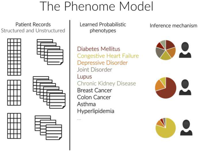
There are two outputs to the UPhenome model: learned phenotypes and an inference mechanism to identify a specific phenotype distribution for an unseen patient record. The learned phenotypes can act as computational models of disease, and can be evaluated according to their interpretability and clinical relevance. In addition, the top-ranked diagnosis for a given phenotype can be used as a label proxy, thus supporting the interpretability of the disease model.

The inference mechanism acts as a dimension reduction technique, where each new patient record can now be represented as a distribution over a concise set of clinically meaningful variables (the learned phenotypes). Such a representation can be leveraged in many health analytics tasks, including patient record summarization, risk prediction, and patient cohort selection. The variables of the model are listed in Table 1.

Table 1:

Variables in the UPhenome model.

P	Number of phenotypes
R	Number of patient records
βr	Phenotype distribution for patient record r
ηp	Diagnosis code distribution for phenotype p
Ir	Number of diagnosis codes in record r
vi,r	Diagnosis code instance i in record r
γi,r	Phenotype assignment for diagnosis code i in record r
θp	Words distribution for phenotype p
Nr	Number of words in record r
wn,r	Word instance n in record r
δn,r	Phenotype assignment for word n in record r
lp	Medications distribution for phenotype p
Or	Number of medication orders in record r
xo,r	Medication instance o in record r
ϵo,r	Phenotype assignment for medication o in record r
kp	Laboratory test distribution for phenotype p
Mr	Number of laboratory tests in record r
ym,r	Laboratory test instance m in record r
ζm,r	Phenotype assignment for test m in record r

3.2. Baseline Models

Before describing the UPhenome model, we first describe two baseline models. The first baseline, LDA-text, considers only the notes in the records, following the hypothesis that clinical information about the diseases of a patient will be documented in the notes and thus can be captured through standard topic modeling. This is a state-of-the-art approach in several models for clinical data [21, 23]. Our first baseline is thus a vanilla LDA applied to the bag of words in the notes. We ran preliminary experiments with LDA on only diagnosis codes (similar to the method used by Chen et al. [24]) but chose to focus the discussion on LDA-text given our task of large-scale disease modeling and the abundance of words in the patient records.

The second baseline, LDA-all, learns topic models based on all observations in the record (words, medications, diagnosis codes, and laboratory tests). In this baseline we apply a vanilla LDA on all observation types in a single bag. The working hypothesis for this baseline is that diseases can be represented across the different data types in the record. This baseline model has the exact same input as the UPhenome model.

3.3. Graphical Model

In the UPhenome model, a patient record is represented as a probabilistic mixture of phenotypes, and the phenotypes are defined as a mixture of characteristics derived from a large, diverse population of patients. A phenotype is defined as a set of distributions over the observation vocabularies, one for each of the four heterogeneous data types. As in the LDA baselines, we model the observations and phenotype assignments as multinomial distributions, and the phenotype distributions as sets of Dirichlet distributions. The details of the probabilistic latent variable model are shown in Figure 1 and Algorithm 1. For completeness, I_r, N_r, O_r, M_r etc. are assumed to be Poisson distributed but in practice this does not influence inference as these are fixed quantities.

Figure 1:

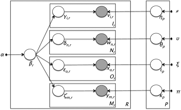
Graphical representation of the UPhenome model.

The UPhenome model departs from the LDA-text baseline by considering all data types in the record. It departs from the LDA-all baseline by treating each data type on its own, and learning the type-specific phenotype distribution separately (η_p, θ_p, l_p, k_p variables). There are multiple advantages to treating the data types this way: (i) this formulation adheres to the genre and characteristic of EHRs; (ii) it allows for future specification of different levels of sparsity and distributions for each data types; (iii) it enables a platform for incorporating domain knowledge specific to each data type; and (iv) it enforces the principle that conditioned on phenotype assignments, the per-data phenotype distributions are independent of each other. Since the four phenotype distributions must separately sum to one, this mitigates potential imbalance in data type prevalence, and thus hinders one frequent observation type (e.g., words) from overwhelming the less frequent ones (e.g., diagnosis codes).

Algorithm 1:

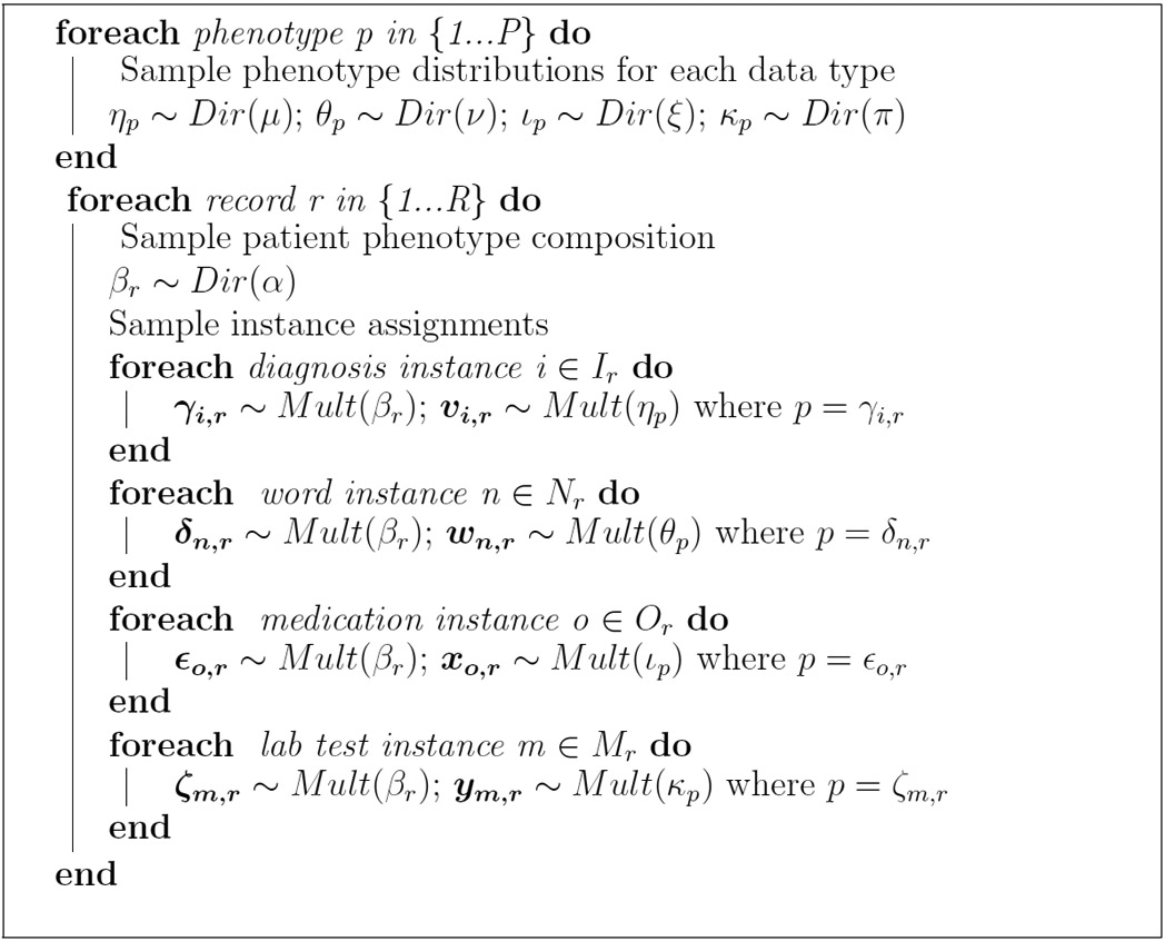
Generative story for the UPhenome model.

3.4. Inference

To perform inference on the UPhenome model, we derived a collapsed Gibbs sampler which collapses the parameters β, η, θ, l, k. Due to the similarity of the models, inference in the UPhenome model follows methods previously outlined for inference in LDA [33]. For illustrative purposes, we show the conditional distribution necessary for Gibbs sampling for one of the phenotype assignment variables, the laboratory test phenotype assignment, and note that the conditionals for the other phenotype assignment variables follow closely.

$$\begin{gathered} p({\zeta }_{m,r}=p\mid {\zeta }_{-(m,r)},\dots )\propto \frac{\left(\pi +{\sum }_{r=1}^R{M}_{r,p,l^{\ast }}^{-(m,r)}\right)}{{\sum }_{l=1}^{\mid \kappa \mid }\left({\pi }_l+{\sum }_{r=1}^R{M}_{r,p,l}^{-(m,r)}\right)}\times \\ \left(\alpha +I_{r,p}+N_{r,p}+O_{r,p}+M_{r,p,l}^{-(m,r)}\right). \end{gathered}$$

Here, the notation I_r,p represents the total count of all diagnosis code tokens I_r in patient record r, that are assigned to phenotype p. Similarly for N_r,p (word tokens) and O_r,p (medications).

The counts for laboratory tests are performed without counting the particular laboratory test instance, m, which belongs to the type l* and for which the conditional distribution is being evaluated. Therefore, $M_{r,p,l^{\ast }}^{-(m,r)}$ represents the total count of all laboratory tests, M_r, in patient record r, that are assigned to phenotype p, except (represented by a minus) for the current laboratory test instance m in record r.

Finally, we note that the denominator of this conditional only contains counts for the laboratory test, demonstrating the differences across the phenotype distributions for each data type.

4. Experimental Setup

We now describe our datasets, parameter settings and model selection, as well as the different evaluation experiments we carried out. Code is available at www.github.com/rimmap/Phenome_Model.

4.1. Datasets

To investigate the generalizability of the UPhenome model, we experimented with two qualitatively different mixtures of patients and patient diseases: (1) records of extremely sick patients who are in the intensive care unit (ICU) with constant monitoring, which usually spans a few days; and (2) records for outpatients regularly followed by care providers over multiple years. These datasets are also from different institutions using different EHR systems. In each dataset, 80% of the records were used for training, and 20% for testing. Descriptive statistics about the training sets for each dataset are given in Table 2.

Table 2:

Descriptive statistics for the MIMIC and NYPH training datasets. In this work, the number of patients and the number of input records is equivalent. Each MIMIC patient has one input record consisting of all data gathered during one ICU stay and each NYPH patient has one input record consisting of all data gathered during four consecutive outpatient visits.

Data Type	MIMIC Total / Unique	NYPH Total / Unique
Patients	18,697 / 18,697	9,828 / 9,828
Words	13,086,278 /12,919	13,494,149 /13,158
Medications	1,044,541 / 855	9,978 / 273
Lab Tests	7,499,446 / 309	351,992 / 300
Diagnoses	159,740 / 985	177,420 / 931

MIMIC II ICU Dataset.

The MIMIC II Clinical Database (v2.26) [34] is available at http://physionet.org/mimic2_clinical_overview.shtml. MIMIC II contains a de-identified set of over 23,000 adults from the Beth Israel Deaconess Medical Center’s Intensive Care Units, including medical, surgical, and coronary care units. The dataset contains structured record data, and unstructured clinical note data. Patients have a broad set of existing conditions and reasons for being in the ICU. As this dataset is available to researchers who sign a data usage agreement, any work on this dataset can serve as a benchmark for future automated phenotyping algorithms.

We included all adult patients in the dataset, independently of their present or absent conditions. For each record, we selected one ICU admission and all of its corresponding observations: discharge summary, all medications, all diagnosis codes, and all laboratory tests. Medications and laboratory tests were mapped to the standard vocabulary definitions provided by MIMIC. For all data types, we limited the vocabulary to observations that appeared at least 20 times across the entire training dataset.

NewYork-Presbyterian Hospital Outpatient Dataset.

The NewYork-Presbyterian Hospital (NYPH) outpatient dataset contains longitudinal records of patients with at least three outpatient visits (e.g., specialist or primary care provider). Their records include all their visits, however, ranging from outpatient visits to hospital admissions, to emergency department visits. Like the MIMIC patients, the NYPH patients have a broad set of conditions, but unlike them their records span years instead of days, and the documented conditions differ as well.

We included all patients, independently of their conditions. Since their records span decades and often hundreds of visits, we considered slices of records for each patient that capture a somewhat stable health status (thus again, making for a qualitatively different dataset than the MIMIC patients). We selected the most recent time slice of each record, that contained four different primary provider notes with no intervening inpatient stays. We defined record lengths by number of notes and not absolute time to account for different rates of visit. Any patient whose record slice lasted less than 1 month or greater than 4 years was removed and this resulted in patient records with mean length of 10 months (7 months standard deviation).

Like in MIMIC, we collected all observations related to primary provider notes, medications, diagnosis codes, and laboratory tests. The range of medications is much more diverse than MIMIC medications, and thus we mapped all medications to their therapeutic class when possible (e.g., “Tylenol” was mapped to “Analgesic”). Similarly, the laboratory tests were mapped to groups of tests when possible (e.g., “Glucose fingerstick” was mapped to “Glucose”). Thus, the vocabulary sizes for these observations was dramatically reduced. We applied frequency thresholds to the data to closely match MIMIC vocabulary sizes whenever possible.

IRB approval was obtained from the Columbia University Medical Center Institutional Review Board. As part of the approved IRB protocol, an application for waiver of authorization was filled and approved, as we investigate algorithms for learning statistical models across a very large population and historical data across many years, and thus obtaining individual consent would be impracticable.

4.2. Model Parameters and Model Selection

We ran UPhenome using 50, 75, 100, 250, 500, 750 phenotypes. All of the hyperparameters (α, μ, ν, ξ, π) were set to 0.1 for all models. To ensure appropriate burn-in time for each model, the Gibbs sampler was run 7,000 iterations and the log-likelihood curves on training data were examined to verify burn-in. The learned phenotype assignment settings for each model were selected as the ones that produced the maximum log-likelihood over all 7,000 iterations on the training set.

For model selection, we optimized for interpretability of phenotypes, and thus relied on both held-out likelihood and coherence of the learned phenotypes. The automated phenotype coherence calculation was performed using normalized pointwise mutual information (NPMI) over all observation types, as described by Lau et al [32] and using the provided open source code. For each model, we used the average NPMI across all phenotypes to represent the overall coherence of the learned phenotypes from the model.

For this experiment, NPMI is calculated for each observation (z_i) in each phenotype, limited to the top 40 (N=40) most probable observations. The per-phenotype NPMI is the average of the NPMI of each observation that is associated with that phenotype. The model NPMI is the average of each per-phenotype NPMI value and is defined by

$$NPMI(z_i)=-\sum _{j=1}^{N-1}\frac{log\frac{P(z_i,z_j)}{P(z_i)P(z_j)}}{\log P(z_i,z_j)},$$

where P(z_i) = probability of seeing observation z_i and P(z_i,z_j) = probability of seeing both observation z_i and observation z_j in the same patient record.

To calculate the likelihood on the held-out set, we implemented a Chib-style estimator as described by Murray and Salakhutdinov[35]. The likelihood was calculated using 1,000 iterations of the estimator for every setting of P.

The combination of the two metrics suggested that P=250 was likely to produce the best phenotypes given the current parameter settings on the MIMIC dataset. We report results on the NYPH dataset that are also obtained with P=250 as well.

For both baseline models LDA-text and LDA-all, we used the MALLET software package[36] with similar number of topics as the selected UPhenome model (K=250) and similarly with 7,000 iterations to ensure burn-in. The hyperparameter settings for the baseline models were 0.01 to increase sparsity due to the larger size of the combined vocabulary.

4.3. Evaluation Experiments

In addition to the automated evaluation metrics, such as held-out likelihood and automatic coherence of the learned phenotypes, we carried out the following set of experiments: qualitative assessment of learned phenotypes (manual coherence, manual granularity, pairwise phenotype comparison, label quality) and ability of the phenotypes to characterize ground-truth disorders present in a set of unseen patients (disorders to phenotypes associations).

All qualitative judgments were obtained from a clinical expert. The learned phenotypes were displayed using a modified version of the interactive topic modeling interface [37]. The interface is particularly useful to us because it enables users to edit learned phenotypes by adding/removing observations and marking them as important or ignorable. For each phenotype, the top 40 most probable observations were displayed and weighted by their phenotype probability (normalized by their data-type specific phenotype probability). The observations were also color-coded to signify their data types (purple for words, grey for medications, green for laboratory tests, and blue for diagnosis codes). See Figure 2 for an example of displayed topic.

Figure 2:

An example of learned phenotype from the NYPH dataset. The top-40 most probable observations for the phenotype are listed. Words are purple, laboratory tests are green, medications are grey, and diagnosis codes are blue.

Manual coherence.

This experiment allows us to capture the intrinsic quality of the learned phenotypes across its probable observations, very much like the automatic coherence metric aims to. In our case, a coherent phenotype is one that describes a single condition and that does not contain observations that are not typically seen in patients with this condition.

For the UPhenome model and the baseline LDA-all model each, 50 phenotypes were randomly selected and presented one at a time to the clinical expert. The expert was asked to score the coherence of a given phenotype (without being told whether it was produced by the LDA-all or UPhenome) according to a 1-5 Likert scale, where 1 designated no coherence (i.e., a junk phenotype) and 5, perfect coherence. To help the expert in his assessment, we instructed him to use the interface to edit the phenotypes, and use his number of edits as a cue for lack of coherence.

Manual granularity.

Because both the baseline and the UPhenome models are unsupervised, there is no guarantee that the learned phenotypes are good representations of clinically meaningful diseases. In particular, it is possible that the modeling of patient observations generates clusters that are reflective of the documentation processes of healthcare rather than of the documentation of clinical status of a patient. For instance, patient discharge to a nursing home in the MIMIC dataset contains very specific documentation patterns, which in an unsupervised setting could be easily grouped.

We asked the clinical expert to categorize the 100 random phenotypes (50 from the UPhenome model and 50 from the LDA-all baseline) into one of the following three granularities: (i) a non-disease phenotype (e.g., a documentation phenotype, or a junk phenotype); (ii) a mix of diseases; (iii) a single disease.

Pairwise phenotype comparison.

In this experiment, we assess the compared overall quality between the learned UPhenome phenotypes and learned LDA-baselines phenotypes. To ensure that the comparison is fair, we selected the 50 random UPhenome phenotypes, and identified the most similar corresponding LDA-all phenotype for each. To compute pairwise phenotype similarity, we used Jensen-Shannon divergence over the posterior probabilities of all observations [38]. The clinical expert was presented pairs of phenotypes (a UPhenome and a paired LDA-baselines phenotype) without him knowing which model generated which phenotype. The expert was asked to choose which phenotype was more clinically coherent or to code the comparison as impossible when both phenotypes were junk, equivalent, or paired improperly.

Label quality.

One of the data types used in the UPhenome model is diagnosis codes. The diagnosis codes are ICD-9 codes, which often describe specific diseases (e.g., “breast cancer”), but can also describe classes of diseases (e.g., “malignant neoplasms”), as well as generic statements about a patient (e.g., “personal history of other diseases”). Since the diagnosis codes are often used in the clinical world as proxies for conditions present in a patient, this experiment assesses to which extent the most probable diagnosis code for a learned phenotype is a clinically appropriate label for the phenotype as a whole.

Since the LDA-text baseline does not include diagnosis codes, so this experiment was skipped for this model. Similarly, since in the baseline LDA-all model it is possible that the top-40 most probable observations do not include any diagnosis code (in our experiment, this happened actually very often), we assessed label quality for the 50 UPhenome phenotypes only.

We asked the clinical expert to categorize the top diagnosis code with respect to the phenotype as a whole as (i) related; (ii) unrelated; or (iii) actionable. An actionable label is one that accurately represents the phenotype at the right granularity and it can be relied upon when making a decision about a patient with the phenotype assigned.

Disorders to phenotypes associations.

While the previous experiments assessed the quality of the learned phenotypes, this experiment assesses the ability of the UPhenome phenotypes to characterize clinically relevant and ground-truth disorders present in a set of unseen patient records. If there is a strong association between phenotypes and the disorders in these records, then the phenotypes can be considered clinically relevant for a given patient.

A potential application of the UPhenome model to identify present disorders for a given patient by inferring the most probable phenotypes for the record. To validate this point, we relied on a gold-standard set of records, which contain manual annotations of the disorders present and mentioned in the records’ notes. The ShARe gold standard is based on MIMIC notes and contains such annotations [39, 40]. We included the 350 discharge summaries from the ShARe corpus in our test set. For each record, gold-standard annotation provided a list of SNOMED-CT Disorder concepts, along with modifiers such as negation and uncertainty [12, 41]. Ground-truth disorders for a record were defined as concepts with no negation or uncertainty.

In total, for each of the 350 records, we have ground-truth disorder concepts (from a set of 2,000+ unique concepts in the corpus) and inferred phenotype assignments. We created an association matrix, similar to [33], visualizing the degree of association between present concepts and phenotypes. We selected the concepts which occurred in at least 50 records. This experiment examines associations between common disorders and learned phenotypes; with 350 patients, there are not enough annotations to associate phenotypes with rare disorders. The association was computed using normalized pointwise mutual information, and for each concept the top phenotype was selected.

5. Results

Figure 2 shows an example of learned phenotype on the NYPH dataset. The label on the left is the most probable diagnosis code, in this case SLE (Systematic Lupus Erythematosus). The words (in purple) are indeed related to this disease and refer to abbreviations in clinical notes (“rheum”) or mentions of important laboratory tests for SLE (“ana”, “esr”), as well as mentions of specific drugs indicated for SLE (“plaquenil”). The medications are also related (plaquenil, one of the most common drug for SLE is an antimalarial medication), as well as prednisone. Both C3 and C4 levels are used as diagnosis tests for SLE, while ESR and others test for level of inflammation in a patient. SLE is a phenotype learned from the NYPH dataset, which represents outpatient records over long periods of time. Since SLE is a chronic disease it makes sense that it was discovered in this dataset. For comparison, there is no phenotype learned on the MIMIC dataset that captures characteristics of SLE. Because the UPhenome model is unsupervised, it models the diseases that are of interest to a given input clinical setting/patient cohort.

For the remainder of the paper, we present results of our experiments on the publicly available MIMIC dataset. Furthermore, for the comparison of the UPhenome model with baselines, we report its comparison to the LDA-all baseline alone, but note that the results were similar as for the comparison to the LDA-text baseline.

Manual coherence.

Figure 3 shows the distribution of coherence scores for the 50 phenotypes from the UPhenome model and the 50 phenotypes from the LDA-all model. The LDA-all phenotypes contained many more junk phenotypes than the UPhenome ones, and at the same time contained slightly more perfectly coherent phenotypes than the UPhenome ones. Overall, about 66% of the UPhenome phenotypes were scored as good (coherence score above 4), while only about 52% of the LDA-all phenotypes were scored as good.

Figure 3:

Distribution of manual coherence scores for the UPhenome and LDA-all phenotypes. A score of 1 represents a junk phenotype and 5, a perfect phenotype.

Manual granularity.

The UPhenome model yielded more phenotypes that are clinically well-defined as representing a single disease than the LDA-all baseline. Furthermore, the LDA-all baseline suffered from a high number of junk phenotypes (as confirmed by the Manual coherence experiment).

For the UPhenome phenotypes, the clinical expert categorized 10% as non-disease phenotypes, 10% as a mix of diseases, and 80% as representing a single disease. In contrast, for the LDA-all phenotypes, the clinical expert categorized 42% as non-disease phenotypes, 6% as a mix of diseases, and 52% as representing a single disease.

Pairwise phenotype comparison.

Figure 4 displays an example of paired phenotypes shown to the clinical expert. We can see that the most probable observations in the LDA-all phenotype are words and laboratory tests (except for one medication), with only a few highly probable and relevant words/tests and most irrelevant to iron deficiency anemia. In comparison, the most probable observations in the UPhenome phenotype are spread across data types, with a majority of observations relevant to iron deficiency anemia.

Figure 4:

An example of LDA-all and UPhenome phenotypes, both about Iron Deficiency Anemia, as paired automatically by Jensen Shannon divergence.

Overall, out of the 50 pairs of phenotypes assessed, the clinical expert considered comparison impossible for 9 pairs. The UPhenome phenotype was superior to the LDA-all one in 80.4% of the remaining pairs.

Label quality.

Overall, the most probable diagnosis code for a given phenotype was evaluated as promising proxy for a phenotype label. The clinical expert assigned a label as actionable for 48% of the UPhenome phenotypes, 44% of them were considered related, while only 8% of them were considered unrelated.

Disorders to phenotypes associations.

Figure 5 shows the association matrix between the present disorders in the gold standard ShARe corpus and the inferred phenotypes on the gold-standard records. There were 15 disorder concepts that were present for at least 50 patients in the dataset. As such the matrix is 15x15. For clarity purposes, we grouped the 15 disorder concepts based on each other’s clinical similarities. For instance, hypertension, hypercholesterolemia, and type II diabetes are often seen together in patients, and similarly for the symptoms nausea and vomiting.

Figure 5:

Association of manually identified ground-truth concepts and automatically inferred phenotypes over a set of patients, along with four example phenotypes.

The hgure indicates there is an association between the common disorders present in the gold-standard records and their inferred phenotypes. Upon inspection of the inferred phenotypes, they are good representations of the present disorders. For instance, Phenotype 7 has the highest association with the disorder Mitral Valve Regurgitation, and its most probable observations are perfectly coherent with respect to this disease.

When concepts shared clinical characteristics (e.g., nausea and vomiting or the cluster of hypertension, diabetes, and hypercholesterolemia), the associated phenotypes are also shared amongst them (e.g., phenotypes 12,13 and phenotypes 1,2).

We display two more examples of phenotypes. Phenotype 10, which is associated with hemorrhage shows several diagnosis codes, all potentially leading or describing hemorrhages. Phenotype 11 is a junk topic, containing highly prevalent observations throughout the MIMIC dataset.

6. Discussion

The results of the various automated and manual evaluations suggest that the UPhenome model is a promising approach to discover models of disease. We discuss next two characteristics of our model—the joint modeling of heterogeneous data types and their unsupervised modeling— as well as the differences between automated and manual coherence assessments for the task of phenotyping.

Joint modeling of heterogeneous EHR data.

The UPhenome model is designed to leverage the innate heterogeneity of EHR data. By modeling each data type separately as opposed to a bag of observations like in the LDA-all baseline, the model can accommodate for imbalance of observations from each data type. For instance, there are many more words than diagnosis codes, even after stop words removal and vocabulary filtering. By design, the UPhenome model ensures that each data type is represented in the learned phenotypes, thus truly modeling across data types. This explains for instance, why all UPhenome phenotypes given as examples in the paper have a mix of data types, while most LDA-all phenotypes are overwhelmed by words and laboratory tests (i.e., the most common data types in our observations, as described in Table 2.

Generative unsupervised modeling of EHR data.

Like all unsupervised models, UPhenome is exciting in its ability to discover patterns in input datasets, such as disease models. When applied to the MIMIC corpus, the learned phenotypes are representative of diseases that are documented in an intensive care unit, like acute kidney failure, while when applied to the NYPH dataset, the learned phenotypes are more representative of chronic and acute conditions that do not require intensive care, such as SLE.

Without careful modeling however, unsupervised models can yield unwanted results. The LDA-all phenotypes often highlighted information about hospital course in aspects nonspecific to any underlying condition, such as coagulation status, palliative care status, type of drug exposure, and plan for discharge. All of these topics make sense and represent distinct patterns in the input datasets, but they do not represent diseases. In contrast, the UPhenome phenotypes represented a greater number of distinct disease than the LDA-all phenotypes. Furthermore, they were more clinically relevant, as multiple aspects of a given disease were included such as secondary complications or potential treatments.

In this version of the model, we did not explore the use of different distributions, maybe more adapted to our task. For instance, several learned phenotypes corresponded to highly prevalent diseases (i.e., these diseases had several phenotypes representing them). Potential fixes for this phenomenon include tuning the hyper-parameters [42] and choosing a different distribution for the data-type specific phenotype distributions.

Automated coherence metrics vs. human judgments.

When comparing the average coherence of the LDA-all phenotypes and the UPhenome phenotypes, LDA-all yielded a significantly higher average Normalized Pointwise Mutual Information (NPMI) (.07 vs .014).

NPMI was established as a valuable automated evaluation metric of learned topics and was shown to correlate with human judgments of topic coherence[32]. In our experiments however, we found little correlation between the clinician’s judgments and the NPMI of the learned phenotypes (Pearson R=0.31 and Spearman=0.33 over 50 UPhenome phenotypes). In our settings, the UPhenome model is a mixture model over text but also coded data (e.g., diagnosis codes, medications, and laboratory results). It is possible that the computationally coherent (often co-occurring terms) are not actually clinically relevant. For instance, the LDA-all phenotype with the highest NPMI contained the following most probable observations: “pm total co pt potassium gap sodium urea chloride anion glucose creat hct hgb rbc mcv mchc mch wbc rdw”, a mix of routine, non-discriminatory laboratory tests. It is also possible that different observations within coded data types may not occur frequently together. For instance, there are several diagnosis codes which are highly clinically relevant with each other, and yet do not get coded together in patient records: different stages of pancreatic cancer for example, would make sense in a single phenotype for the disease, but will not be seen jointly over many patients at a time.

7. Conclusion and Future Work

Building computational models of disease has been an active area of research, with approaches ranging from building ontologies and taxonomies of diseases based on clinical expertise, to creating highly precise model of specific diseases of interest through a mix of data-driven and clinical expertise, to discovering models directly from clinical observations. The UPhenome model is an unsupervised, generative model, which given a large set of EHR observations, learns probabilistic phenotypes. The phenotypes are learned jointly over heterogeneous EHR observations drawn from a large set of potential medications, diagnosis codes, laboratory tests, and free-text clinical notes. When applied to specific patient records, the UPhenome model can provide actionable representation of the records, by describing them as a distribution over the patient’s inferred phenotypes.

We demonstrate that the UPhenome model can learn from different care settings and documentations of different healthcare institutions, without any adaptation needed. Our experiments show that the UPhenome model yields phenotypes that (i) combine all these data types in a coherent fashion better than baseline models; (ii) are representative of single diseases, while baseline models tended to produce representations of either mixes of disease or high-level healthcare process; and (iii) when applied to unseen patient records, are correlated with the patients’ ground-truth disorders.

The code for the UPhenome model is available at www.github.com/rimmap/Phenome_Model. Furthermore, the MIMIC dataset is available to the research community.

This paper presents the first iteration of the UPhenome model, which as such makes several simplification assumptions about the data and the task. We describe next our future work to address these current limitations.

Future Work.

We plan our future work along the following directions: (i) temporality of EHR data and diseases; (ii) better modeling of the different data types; and (iii) grounding of the learned phenotypes with clinical knowledge about disease.

In its current version, the UPhenome model does not explicitly encode any temporality about given patient records. Because longitudinal records and diseases themselves are often not time invariant [43], and progress at different time resolutions, it is a non-trivial task to model temporality across all diseases at once. A simple baseline experiment toward incorporating temporality is to infer phenotypes over time, much like the approach of dynamic topic models [44].

Each of the considered data types in the UPhenome model have specific characteristics that can be exploited further. The EHR text, especially when learning from several notes for each patient, has much redundancy that can be accounted for [27]. Medications and diagnosis codes are hierarchical in nature, with evidence that incorporating that structure helps in modeling clinical information [26]. Finally each laboratory test has associated values, and it is clear that different distributions of the same test can describe different diseases; for instance, glucose with a distribution biased towards high values would belong to a phenotype describing diabetes, while glucose with a distribution with mean towards low values would be probable in a hypoglycemia phenotype. Better modeling of the data types based on the genre of EHR datasets is an attractive and promising avenue of research.

In addition to incorporating knowledge about EHR characteristics, we are eager to investigate the use of clinical knowledge in improving probabilistic phenotyping. A primary goal of our work is to generate phenotypes compatible with clinician’s mental models of diseases. Incorporating a human in the loop, like in interactive topic modeling [37] and clinical anchor learning [45] is a promising approach. Another approach to support this goal is to incorporate knowledge from existing clinical knowledge resources, inspired by the advances in constrained topic modeling [46, 47, 37], and incorporating known semantic relations in disease modeling [48, 7].

Highlights.

We present the UPhenome model, which derives phenotypes in an unsupervised manner.

UPhenome scales easily to large sets of diseases and clinical observations.

The learned phenotypes combine clinical text, ICD9 codes, lab tests, and medications.

UPhenome learns phenotypes that can be applied to unseen patient records.

References

- [1].Perotte A, Ranganath R, Hirsch JS, Blei D, Elhadad N, Risk prediction for chronic kidney disease progression using heterogeneous electronic health record data and time series analysis., Journal of the American Medical Informatics Association : JAMIA 22 (4) (2015) 872–880. [DOI] [PMC free article] [PubMed] [Google Scholar]
- [2].Ranganath R, Perotte A, Elhadad N, Blei DM, The Survival Filter: Joint Survival Analysis with a Latent Time Series, UAI. [Google Scholar]
- [3].Wei W-Q, Denny JC, Extracting research-quality phenotypes from electronic health records to support precision medicine., Genome medicine 7 (1) (2015) 41. [DOI] [PMC free article] [PubMed] [Google Scholar]
- [4].Liao KP, Cai T, Savova GK, Murphy SN, Karlson EW, Ananthakrishnan AN, Gainer VS, Shaw SY, Xia Z, Szolovits P, Churchill S, Kohane I, Development of phenotype algorithms using electronic medical records and incorporating natural language processing, BMJ 350 (April24 11) (2015) 1885. [DOI] [PMC free article] [PubMed] [Google Scholar]
- [5].Hripcsak G, Albers DJ, Next-generation phenotyping of electronic health records., JAMIA 20 (1) (2013) 117–121. [DOI] [PMC free article] [PubMed] [Google Scholar]
- [6].Newton KM, Peissig PL, Kho AN, Validation of electronic medical record-based phenotyping algorithms: results and lessons learned from the eMERGE network, JAMIA. [DOI] [PMC free article] [PubMed] [Google Scholar]
- [7].Yu S, Liao KP, Shaw SY, Gainer VS, Churchill SE, Szolovits P, Murphy SN, Kohane IS, Cai T, Toward high-throughput phenotyping: unbiased automated feature extraction and selection from knowledge sources, Journal of the American Medical Informatics Association : JAMIA. [DOI] [PMC free article] [PubMed] [Google Scholar]
- [8].Marlin BM, Kale DC, Khemani RG, Wetzel RC, Unsupervised pattern discovery in electronic health care data using probabilistic clustering models, in: IHI, 2012, pp. 389–398. [Google Scholar]
- [9].Lasko TA, Denny JC, Levy MA, Computational phenotype discovery using unsupervised feature learning over noisy, sparse, and irregular clinical data, PLoS ONE 8 (6) (2013) e66341. [DOI] [PMC free article] [PubMed] [Google Scholar]
- [10].Doshi-Velez F, Ge Y, Kohane I, Comorbidity clusters in autism spectrum disorders: an electronic health record time-series analysis., Pediatrics 133 (1) (2014) e54–63. [DOI] [PMC free article] [PubMed] [Google Scholar]
- [11].Schulam P, Wigley F, Saria S, Clustering longitudinal clinical marker trajectories from electronic health data: Applications to phenotyping and endotype discovery, in: AAAI, 2015. [Google Scholar]
- [12].SNOMED clinical terms, http://www.nlm.nih.gov/research/umls/Snomed/snomed_main.html (2009).
- [13].Miller RA, Pople HE, Myers JD, INTERNIST-1, an experimental computer-based diagnostic consultant for general internal medicine, The New England Journal of Medicine 307 (8) (1982) 468–476. [DOI] [PubMed] [Google Scholar]
- [14].Shwe MA, Middleton B, Heckerman DE, Henrion M, Horvitz EJ, Lehmann HP, Cooper GF, Probabilistic diagnosis using a reformulation of the INTERNIST-1/QMR knowledge base. I. The probabilistic model and inference algorithms., Methods of Information in Medicine 30 (4) (1991) 241–255. [PubMed] [Google Scholar]
- [15].Jaakkola TS, Jordan MI, Variational probabilistic inference and the QMR-DT network, JAIR. [Google Scholar]
- [16].Hidalgo CA, Blumm N, Barabási A-L, Christakis NA, A dynamic network approach for the study of human phenotypes, PLoS computational biology 5 (4) (2009) e1000353. [DOI] [PMC free article] [PubMed] [Google Scholar]
- [17].Hanauer DA, Rhodes DR, Chinnaiyan AM, Exploring clinical associations using ‘-omics’ based enrichment analyses, PLoS ONE 4 (4) (2009) e5203. [DOI] [PMC free article] [PubMed] [Google Scholar]
- [18].Roque FS, Jensen PB, Schmock H, Dalgaard M, Andreatta M, Hansen T, Søeby K, Bredkær S, Juul A, Werge T, Jensen LJ, Brunak S, Using electronic patient records to discover disease correlations and stratify patient cohorts, PLoS Computational Biology 7 (8) (2011) e1002141. [DOI] [PMC free article] [PubMed] [Google Scholar]
- [19].Ho JC, Ghosh J, Sun J, Marble: high-throughput phenotyping from electronic health records via sparse nonnegative tensor factorization, in: KDD, 2014. [Google Scholar]
- [20].Blei D, Ng A, Jordan M, Latent dirichlet allocation, JMLR 3 (2003) 993–1022. [Google Scholar]
- [21].Arnold CW, PhD, El-Saden SM, MD, Bui AA, PhD, Taira R, PhD, Clinical case-based retrieval using latent topic analysis, in: AMIA, 2010. [PMC free article] [PubMed] [Google Scholar]
- [22].Chan KR, Lou X, Karaletsos T, Crosbie C, Gardos S, Artz D, Ratsch G, An empirical analysis of topic modeling for mining cancer clinical notes, in: IEEE ICDMW, 2013. [Google Scholar]
- [23].Ghassemi M, Naumann T, Doshi-Velez F, Brimmer N, Joshi R, Rumshisky A, Szolovits P, Unfolding physiological state, in: KDD, 2014. [DOI] [PMC free article] [PubMed] [Google Scholar]
- [24].Chen Y, Ghosh J, Bejan CA, Gunter CA, Gupta S, Kho A, Liebovitz D, Sun J, Denny J, Malin B, Building bridges across electronic health record systems through inferred phenotypic topics., Journal of Biomedical Informatics (2015) 1–12. [DOI] [PMC free article] [PubMed] [Google Scholar]
- [25].Saria S, Koller D, Penn A, Learning individual and population level traits from clinical temporal data, in: NIPS, 2010. [Google Scholar]
- [26].Perotte AJ, Wood F, Elhadad N, Bartlett N, Hierarchically supervised latent Dirichlet allocation, in: NIPS, 2011. [Google Scholar]
- [27].Cohen R, Aviram I, Elhadad M, Elhadad N, Redundancy-aware topic modeling for patient record notes, PLoS ONE 9 (2) (2014) e87555. [DOI] [PMC free article] [PubMed] [Google Scholar]
- [28].Wang X, Sontag D, Wang F, Unsupervised learning of disease progression models, in: KDD, 2014. [Google Scholar]
- [29].Chang J, Boyd-Graber JL, Gerrish S, Wang C, Blei DM, Reading tea leaves: How humans interpret topic models, in: NIPS, 2009. [Google Scholar]
- [30].Wallach HM, Murray I, Salakhutdinov R, Mimno D, Evaluation methods for topic models, in: ICML, 2009. [Google Scholar]
- [31].Newman D, Lau J, Grieser K, Automatic evaluation of topic coherence, in: ACL, 2010. [Google Scholar]
- [32].Lau JH, Newman D, Baldwin T, Machine reading tea leaves: Automatically evaluating topic coherence and topic model quality, in: ACL, 2014. [Google Scholar]
- [33].Griffiths TL, Steyvers M, Finding scientific topics, PNAS; 101 Suppl 1 (2004) 5228–5235. [DOI] [PMC free article] [PubMed] [Google Scholar]
- [34].Saeed M, Villarroel M, Reisner AT, Clifford G, Lehman L-W, Moody G, Heldt T, Kyaw TH, Moody B, Mark RG, Multiparameter intelligent monitoring in intensive care II (MIMIC-II): A public-access intensive care unit database, Critical Care Medicine 39 (2011) 952–960. [DOI] [PMC free article] [PubMed] [Google Scholar]
- [35].Murray I, Salakhutdinov R, Evaluating probabilities under high-dimensional latent variable models, in: NIPS, 2009. [Google Scholar]
- [36].McCallum A, MALLET: A machine learning for language toolkit, http://www.cs.umass.edu/~mccallum/mallet (2002). [Google Scholar]
- [37].Hu Y, Boyd-Graber J, Satinoff B, Interactive topic modeling, in: ACL, 2011. [Google Scholar]
- [38].Manning CD, Schütze H, Foundations of Statistical Natural Language Processing, MIT Press, Cambridge, MA, USA, 1999. [Google Scholar]
- [39].Pradhan S, Elhadad N, South BR, Martinez D, Christensen L, Vogel A, Suominen H, Chapman WW, Savova G, Evaluating the state of the art in disorder recognition and normalization of the clinical narrative., JAMIA. [DOI] [PMC free article] [PubMed] [Google Scholar]
- [40].Semeval-2015 task 14: Analysis of clinical text, http://alt.qcri.org/semeval2015/task14/ (2015).
- [41].Bodenreider O, The Unified Medical Language System (UMLS): integrating biomedical terminology., Nucleic Acids Research 32 (Database issue) (2004) D267–70. [DOI] [PMC free article] [PubMed] [Google Scholar]
- [42].McCallum A, Mimno DM, Wallach HM, Rethinking LDA: Why priors matter, in: NIPS, 2009. [Google Scholar]
- [43].Pivovarov R, Albers DJ, Sepulveda JL, Elhadad N, Identifying and mitigating biases in EHR laboratory tests., Journal of Biomedical Informatics. [DOI] [PMC free article] [PubMed] [Google Scholar]
- [44].Blei D, Lafferty J, Dynamic topic models, in: ICML, 2006. [Google Scholar]
- [45].Halpern Y, Choi Y, Horng S, Sontag D, Using anchors to estimate clinical state without labeled data, in: AMIA, 2014. [PMC free article] [PubMed] [Google Scholar]
- [46].Andrzejewski D, Zhu X, Craven M, Incorporating domain knowledge into topic modeling via Dirichlet forest priors, in: ICML, 2009. [DOI] [PMC free article] [PubMed] [Google Scholar]
- [47].Andrzejewski D, Zhu X, Craven M, Recht B, A framework for incorporating general domain knowledge into latent Dirichlet allocation using first-order logic, in: IJCAI, 2011. [Google Scholar]
- [48].Doshi-Velez F, Wallace B, Adams R, Graph-sparse LDA: A topic model with structured sparsity, in: arxiv, 2015. [Google Scholar]