Global gradients in intertidal species richness and functional groups

Jakob Thyrring; Lloyd S Peck

doi:10.7554/eLife.64541

. 2021 Mar 19;10:e64541. doi: 10.7554/eLife.64541

Global gradients in intertidal species richness and functional groups

Jakob Thyrring ^1,^2,^3,^4,^5,^✉, Lloyd S Peck ¹

Editors: Detlef Weigel⁶, Detlef Weigel⁷

PMCID: PMC8032391 PMID: 33739285

Abstract

Whether global latitudinal diversity gradients exist in rocky intertidal α-diversity and across functional groups remains unknown. Using literature data from 433 intertidal sites, we investigated α-diversity patterns across 155° of latitude, and whether local-scale or global-scale structuring processes control α-diversity. We, furthermore, investigated how the relative composition of functional groups changes with latitude. α-Diversity differed among hemispheres with a mid-latitudinal peak in the north, and a non-significant unimodal pattern in the south, but there was no support for a tropical-to-polar decrease in α-diversity. Although global-scale drivers had no discernible effect, the local-scale drivers significantly affected α-diversity, and our results reveal that latitudinal diversity gradients are outweighed by local processes. In contrast to α-diversity patterns, species richness of three functional groups (predators, grazers, and suspension feeders) declined with latitude, coinciding with an inverse gradient in algae. Polar and tropical intertidal data were sparse, and more sampling is required to improve knowledge of marine biodiversity.

Research organism: Other

Introduction

The latitudinal diversity gradient in species richness across ecosystems and various functional groups has been a major research topic that has intrigued scientists since at least Darwin, 1859 and Wallace, 1878. Over time, many hypotheses have been proposed to explain this seemingly general ecological pattern in marine and terrestrial ecosystems. Ecological and physical hypotheses dominate the discussions and include drivers such as habitat area, stability, speciation rates, energy availability, and temperature (Willig et al., 2003; Clarke and Gaston, 2006; Edgar et al., 2017). However, the geographic, functional, and taxonomic generality of latitudinal diversity gradients remain lively debated as unimodal, bimodal, and inverse gradients emerge across clades, habitats, and latitudes (Rivadeneira et al., 2002; Waller, 2008; Chaudhary et al., 2016; Kinlock et al., 2018). In the marine realm, latitudinal gradients in some groups have been shown to be closely related to oceanographic covariates, such as water temperature (Roy et al., 2000), yet mammal richness peaks at high latitudes (Grady et al., 2019), and more species have been reported from polar soft-sediment habitats than at many lower latitudes (Vause et al., 2019).

While gradients in species diversity have received most attention, latitudinal changes across different functional groups (evaluated here by food acquisition, see Materials and methods) remain less studied despite their importance for ecosystem functioning. Macroalgal canopies shelter understory species from environmental stress (Krause-Jensen et al., 2016; Sejr et al., 2021), creating protective microhabitats that increase environmental heterogeneity and biodiversity, thereby maintaining a diversified understory assemblages (Bulleri et al., 2002; Watt and Scrosati, 2013; Piazzi et al., 2018). Suspension feeders are important benthic-pelagic energy couplers (Gili and Coma, 1998), and predation is widely accepted as a central structuring process in the composition and abundance of species (Vermeij, 1987; Stanley, 2008). Latitudinal studies have shown that suspension feeders dominate benthic systems in fully marine environments at high latitudes (Gili and Coma, 1998; De Broyer et al., 2014), while diversity of coastal macroalgae peaks at mid-latitudes (Keith et al., 2014), and predation pressure decreases with latitude and depth from shallow shelves to deep oceans (Taylor and Taylor, 1977; Harper and Peck, 2016). Most functional group studies have focused on a narrow set of taxa, and global-scale assemblage-wide investigations encompassing both hemispheres are rare. Thus, studies demonstrating global patterns in various functional groups are needed to understand spatial patterns, biological interactions, and ecosystem resilience to climate change.

Intertidal shores rank as one of the most studied marine habitats and are often seen as harbingers for the effects of climate change and invasive species. Regional-scale intertidal studies have found richness gradients of gastropods along coastlines in the eastern Pacific Ocean (Rivadeneira et al., 2015; Fenberg and Rivadeneira, 2019). However, no latitudinal diversity gradient of gastropods (Miloslavich et al., 2013) or macroalgae (Konar et al., 2010) was found on a global scale across oceans, and assemblage-wide studies have found missing (Blanchette et al., 2008; Cruz-Motta et al., 2010) or inverse (Griffiths and Waller, 2016) gradients. Conflicting and missing gradients suggest that richness is determined by regional or local (and not global) scale processes through biological interactions and small scale overlapping environmental gradients. For example, high habitat heterogeneity creates environmental stress mosaics that are more important in shaping biological patterns than latitudinal environmental gradients (Helmuth et al., 2006; Jurgens and Gaylord, 2018). However, the large-scale intertidal studies necessary to evaluate global-scale patterns and processes are generally missing (but see Cruz-Motta et al., 2010; Miloslavich et al., 2013).

Global assessments of intertidal biodiversity have been hindered by data scarcity from polar intertidal shores, and a lack of estimates of intertidal geographic areas. In fact, only the extent of intertidal mud flats have been quantified on a large scale (Murray et al., 2019). However, in recent decades intertidal diversity data from both polar regions have advanced (Weslawski et al., 2010; Griffiths and Waller, 2016; Thyrring et al., 2017; Thyrring et al., 2021; Peck, 2018), providing novel opportunities to study biodiversity patterns and variation in specific functional groups on a worldwide scale. In this study, we examined latitudinal diversity gradients in local intertidal species richness (termed α-diversity) and four functional groups from 433 locations throughout the northern and southern hemispheres, from the high Arctic to the Antarctic. Intertidal ecosystems comprises a variety of habitats ranging from tidal flats to mangrove forests, each supporting unique communities and taxa. Therefore, to control for habitat effects, we specifically focus on rocky shores and boulder fields, as they represent the most studied intertidal habitats and are present in all oceans. We aim to examine patterns in intertidal α-diversity and functional groups across 155° of latitude, and test the following hypotheses: (1) α-diversity decreases with increasing latitude, as evident in other ecosystems and (2) biodiversity is predicted by local-scale structuring processes rather than global-scale oceanographic features.

Results

Latitudinal α-diversity gradients

We extracted data from 433 intertidal sites between 74.8°S and 80.5°N (Figure 1). Only 11 sites were located at latitudes above 70°, south and north combined (Supplementary file 1). A generalized additive mixed effect model (GAMM) indicated a non-linear relationship among α-diversity and latitude in the northern hemisphere where α-diversity peaked at mid-latitudes between 30 and 55°N (GAMM, edf = 2.005, p=0.023). While no latitudinal scale environmental driver was significant (Table 1), α-diversity was similar in the tropical and Arctic regions (Figure 2). In the southern hemisphere, a generalized linear mixed effect model (GLMM) indicated that α-diversity was not related to any latitudinal scale environmental drivers (Table 1), and displayed a linear latitudinal pattern with a non-significant slight decline at the highest latitude (Table 1; Figure 2).

Table 1. Results of the mixed effect models for rocky intertidal α-diversity.

The estimate, standard error (SE), z-value, and p-value are presented for each variable. The estimated degree of freedom (ed), and p-value are presented for the smoother in the northern hemisphere*.

	Estimates	SE	z-Value	p-Value
Northern hemisphere
(Intercept)	3.086	0.283	10.92	<0.001
Chlorophyll a	−0.004	0.088	0.05	0.959
Phosphate	−0.163	0.288	−0.56	0.573
Sea temperature	0.024	0.015	1.64	0.101
Southern hemisphere
(Intercept)	3.199	0.443	7.225	<0.001
Latitude	0.006	0.007	0.899	0.369
Chlorophyll a	−0.006	0.007	−0.829	0.407
Phosphate	−0.240	0.234	−1.029	0.303
Sea temperature	−0.010	0.016	−0.653	0.514

Open in a new tab

*Approximate significance of cubic spline regression smoother: Estimated df = 2.005, p-value=0.023.

Figure 2. — Data are split into southern and northern hemispheres. A linear regression line (southern hemisphere) and a best-fit locally weighted scatterplot smoother (northern hemisphere) was added with 95% confidence intervals to aid visual interpretation.

Local-scale models revealed significant relationships between α-diversity and the four local-scale variates ice scour, macroalgal canopy cover, salinity, and wave exposure (Table 2). We focused exclusively on canopy-forming algae because canopies provide living space and protection from predation and extreme temperatures, thereby increasing α-diversity and coverage of understory organisms. A positive relationship was identified between α-diversity and salinity and macroalgal cover (Figure 3a,c), with salinity having the strongest effect (R² = 0.19, 95% CI = 4.82–8.52, Figure 4). Wave exposure and ice scour had negative effects on α-diversity (Figure 3b,d). The non-linear relationship between wave exposure and α-diversity showed that high levels of wave exposure were necessary to affect levels of α-diversity (Figure 3b). Fewer species inhabited ice-scoured shores compared to ice-free shores (95% CI = −0.57 – −0.23, Table 2), although the model only explained around 5% (R² = 0.05) of the variation due to large differences in the number of species on both ice-scoured and ice-free shores (Figure 3c).

Table 2. Local-scale model summaries with individual models indicated for each model.

Estimated parameters, standard error (SE), bootstrapped 95% confidence intervals (95% CI), z-values, and p-values are reported for the relationship between α-diversity and environmental covariates.

Salinity R² = 0.19 (GLM)
	Estimates	SE	95% CI	z-Value	p-Value
(Intercept)	−3.201	0.891	−4.94; −1.47	−3.6	<0.0001
Salinity	6.676	0.946	4.82; 8.52	7.06	<0.0001
Wave exposure (GAM) R² = 0.12
	Estimates	SE		z-Value	p-Value
(Intercept)*	2.435	0.029		82.4	<0.0001
Ice scour (GLM) R² = 0.05
	Estimates	SE	95% CI	z-Value	p-Value
(Intercept)	2.353	0.055	2.24; 2.46	42.7	<0.0001
Ice scour	−0.401	0.087	−0.57; −0.23	−4.59	<0.0001
Macroalgal cover (GLM) R² = 0.14
	Estimates	SE	95% CI	z-Value	p-Value
(Intercept)	6.133	0.386	5.37; 6.89	15.9	<0.0001
Cover	−2.35	0.547	−3.42; −1.28	−4.3	<0.0001

Open in a new tab

*Approximate significance of locally weighted scatterplot wave exposure smoother: Estimated df = 8.40, p-value<0.0001.

Figure 3. — A best-fit locally weighted scatterplot smoother (LOESS) and 95% confidence intervals (panel b) and boxplots (panels **c,d**) has been added to aid visual interpretation.

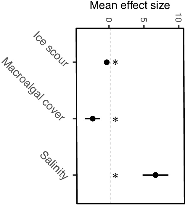
Figure 4. — Significance of regression parameters is identified as bootstrapped 95% confidence intervals (error bars) not crossing zero (* indicates significance).

Latitudinal gradients in functional groups

Four studied functional groups (algae, grazers, predators, and suspension feeders) displayed different latitudinal patterns (Figure 5). Predators, grazers, and suspension feeders declined with latitude in both hemispheres, coinciding with an increase in algal richness (Figure 5). In general, the relative distribution of the functional groups changed faster across latitudes in the southern hemisphere where rapid changes were observed around 20°S, while northern hemisphere communities were more consistent from 25 to 60°N (Figure 5). We were unable to describe functional groups at latitudes 15–25°N as no data were available (indicated as white bars in Figure 5).

In the southern hemisphere, the proportion of predators and grazers declined beyond around 20°S, together forming 6.9% (±6.6 s.d.) of species accounted for between 20 and 55°S, but constituting 18.3% (±15.1 s.d.) of species in communities at latitudes less than 20°S (Figure 5). Suspension feeders were common in low- to mid-latitudes, constituting 34.6% (±9.6 s.d.) of the species present between 20 and 45°S (Figure 5). The relative proportion of algal species increased with latitude, with a small decline at sites between 60 and 65°S (Figure 5). In the northern hemisphere, predators were abundant at low- and mid-latitudes, accounting on average for 18.2% (±5.8 s.d.) of the populations from 0 to 60°N, before declining to 4.7% (±4.1 s.d.) at high latitudes between 61 and 80°N. The number of grazers decreased markedly from around 15°N, but stabilized at 25.4% (±6.4 s.d.) across 25°–80°N (Figure 5). Suspension feeders were the dominant functional group on shores in the northern hemisphere, especially between 25 and 60°N, but decreased to 21.4% (±1.8 s.d.) at high latitudes between 60 and 80°N (Figure 5). Algal species was the most dominant group at high latitudes (Figure 5). In both hemispheres, the assemblage composition at the highest latitudes was substantially different from elsewhere; on these high polar shores, suspension feeders were absent and only a few predators were present, while grazers and algae dominated.

Discussion

Latitudinal α-diversity gradients

Latitudinal diversity gradients have been recognized for centuries, and the generality of this phenomenon has been investigated ever since. Recent state-of-the-art meta-analyses have provided support for latitudinal gradients in various marine and terrestrial ecosystems (Hillebrand, 2004; Kinlock et al., 2018), and latitudinal gradients in assemblage composition and biological interactions have also been identified (Qian and Ricklefs, 2007; Schemske et al., 2009; Harper and Peck, 2016). Although latitudinal diversity gradients are widely quoted as one of the basic laws in ecology (Lomolino, 2004), studies investigating these patterns on a global scale have largely overlooked intertidal ecosystems, despite their global range and importance as unique environments. An intertidal study in the north eastern Pacific Ocean has reported no latitudinal gradients in species richness (Blanchette et al., 2008). It has been suggested that the latitudinal diversity gradient is biogeographically structured (Roy et al., 1994), and since the above investigations were conducted in a temperate biogeographic region, diversity gradients might not occur. For example, while gastropod richness is relatively stable in the temperate region, a steep rise in richness occurs in the tropical region (Fenberg and Rivadeneira, 2019). However, the few published global-scale intertidal studies have revealed contradictory latitudinal patterns with richness of macroalgae (Konar et al., 2010) and small echinoderms peaking at higher latitudes, while large echinoderms peaking at low latitudes (Iken et al., 2010). Consequently, no latitudinal trend in intertidal diversity was demonstrated across 13 marine regions, as overall assemblage richness was similar everywhere despite strong species-specific patterns (Cruz-Motta et al., 2010). While the studies above benefited from analyzing data collected using a standardized protocol across latitudes, they were limited by only including a smaller number of sampling sites (~70 sites), which may have restricted their capacity to demonstrate large-scale trends, or to separate these from locally entrained patterns. Compared to these studies, we expanded the spatial resolution sixfold and present α-diversity data from 433 rocky shore sites across 155° of latitude, yet there was still no support for the latitudinal α-diversity gradient hypothesis. Latitudinal patterns were, however, markedly different between hemispheres, with a mid-latitude peak in the north and a non-significant unimodal trend in the south. We also demonstrated that different functional groups had different patterns (see later discussion).

Northern hemisphere α-diversity displayed a distinct mid-latitude peak, a pattern also reported for open water biodiversity (Chaudhary et al., 2016). The cause behind this remains elusive but hypotheses include a mid-dominance effect where high- and low-latitude species ranges overlap (Powell et al., 2012), and that high temperatures near the equator, and low temperatures and ice cover at the poles, may limit diversity outside of the temperate zone. However, we did not see this pattern in the temperate zone in the southern hemisphere, and we show that water temperatures do not control intertidal α-diversity. Instead, the open water mid-latitudinal richness peak has recently been suggested to be an artifact of limited sampling in less studied tropical regions (Menegotto and Rangel, 2018). This asymmetric sampling holds true for the northern hemisphere rocky intertidal ecosystem as well. While we show data from 11 sites at latitudes above 70° (south and north combined), 44% (n = 193) of all studies were from mid-latitude rocky shores in Europe and North America between 24 and 60°N. Data from low-latitude regions is furthermore limited because rocky shorelines are scarce in the tropics (Fenberg and Rivadeneira, 2019), and the majority of tropical studies have focused on specific taxonomic groups, and not assemblage-wide patterns (e.g., Hartnoll, 1976; Chelazzi and Vannini, 1980; Mille-Pagaza et al., 2002; Konar et al., 2010; Flores-Rodríguez et al., 2014; Rivadeneira et al., 2015; Gbedemah, 2017; Hendrickx et al., 2019, but see Lourenço et al., 2020). Thus, mid-latitudinal rocky shores, especially in the northern hemisphere, are among the most sampled globally, and future tropical collections may change understanding of biodiversity patterns. This disproportionate sampling pattern is also present in other marine habitats, where sampling intensity is highest at mid-latitudes in the northern hemisphere (Menegotto and Rangel, 2018). Polar data were also limited in the southern hemisphere where species diversity was relatively constant across latitudes with a non-significant dip at the highest latitude. A factor that powerfully affects intertidal diversity in the high polar regions is that most intertidal areas are encased in ice for large parts, if not all of the year, which reduces intertidal biodiversity to zero in these areas. Thus, the Arctic permafrost coastline represents around 34% of the world’s coastline (Lantuit et al., 2012), and Antarctica accounts for around 2.7% (45,317 km). However, in the Antarctic only around 12% of that is ice-free in summer (5468 km) and at both poles much less, if any, is ice-free in winter (Peck, 2018). This lack of ice-free intertidal areas in high polar sites restricts the capacity for communities to establish, and limits the development of macroalgal species (Miller and Pearse, 1991; Mystikou et al., 2014). However, high polar shores are seldom studied (Thyrring et al., 2021), and in this study high-latitude Antarctic shorelines were only represented by a single study at a single site, thus this depression in number of species should be interpreted with caution. In ice-free areas, and at lower Antarctic latitudes, previous biodiversity studies have shown intertidal species richness to increase with latitude from the southern Atlantic ocean to the Antarctic Peninsula (Waller, 2008; Griffiths and Waller, 2016). The situation is clearly complex and, in general, more information on the influence of geographic sampling biases across latitudes are, together with more data from more sites, especially the polar and tropical regions, required to understand and model large-scale biodiversity patterns.

Latitudinal diversity gradients have been identified in subtidal habitats (e.g., Roy et al., 2000; Edgar et al., 2017), and the contrasting patterns in biodiversity gradients between intertidal and subtidal ecosystems may originate from differences in the factors controlling α-diversity. Subtidal benthic habitats experience relatively homogenous environmental conditions across small-to-moderate spatial scales, and large-scale latitudinal diversity gradients are therefore less impacted by local factors and reflect larger-scale changes in environmental conditions. For instance, decreasing water temperatures profoundly affect physiological performance of marine ectotherms (e.g., growth, reproduction and activity, muscle performance) and special adaptations are required to live in cold waters (Peck, 2016; Peck, 2018). Latitudinal biodiversity gradients in ectotherms have, therefore, been attributed to changes in water temperatures in subtidal habitats (Roy et al., 2000; Edgar et al., 2017). Our data run contrary to this and indicate that organisms inhabiting the intertidal do not conform to classic LDG patterns, or any of the correlated environmental drivers (e.g., water temperature). Instead, we demonstrate significant effects of local-scale variation in salinity, wave exposure, ice scour, and biogenic habitats (i.e., macroalgal canopy cover), indicating that α-diversity is determined by small-scale processes through biological interactions and overlapping environmental gradients. Indeed, the importance of microhabitats; biological interactions; and local physical parameters on intertidal community assemblage, density, and diversity has been studied extensively on rocky intertidal shores (Paine, 1974; Archambault and Bourget, 1996; Coleman et al., 2006; Scrosati and Heaven, 2007; Piazzi et al., 2018; Sejr et al., 2021), and high spatial variable in intertidal community coverage and structure between closely adjacent areas are well known (Underwood and Chapman, 1996; Benedetti-Cecchi and Cinelli, 1997; Sejr et al., 2021). For example, algal canopies provide food, predation refugium, and a moist understory environment where species sensitive to desiccation stress can survive during low tides (Dayton, 1975), thus the understory community may be rich and distinct from the surrounding open shoreline (Benedetti-Cecchi et al., 2001; Bulleri et al., 2002; Watt and Scrosati, 2013). Canopies and surface topography also shelter organisms from extreme air temperatures, thereby increasing local coverage and diversity, and facilitating recolonization of the substrate by secondary species (Blanchard and Bourget, 1999; Watt and Scrosati, 2013; Ørberg et al., 2018). Moreover, wave exposure decreases diversity, especially at high latitude where floating ice is pushed on the shore by waves, amplifying the impacts of ice scour on exposed coastlines (Scrosati and Heaven, 2007). Even wave splashing and low water timing (i.e., low tides occurring in the tropics during the hottest time of the day are more harmful than low tides in the middle of the night [Helmuth et al., 2002]) have been shown to be important. All these factors interact and change in non-latitudinally related patterns, creating highly localized unique environmental conditions that, in combination, functionally override latitudinal stress or energy gradients. Thus, although the strength and direction of environmental stressors change across latitudes (i.e., from ice scour and extreme sub-zero temperature in polar regions to desiccation and acute heat stress in the tropics), the combined stress experienced by resident populations may roughly balance out across most latitudes and produce no clear gradient. In a recent study in South America, α-diversity generally did not conform to latitudinal diversity gradient predictions for either the Atlantic or Pacific coast (Cruz‐Motta et al., 2020), and we demonstrate similar patterns on a global scale. A conclusion from this research is that instead of focusing on large-scale drivers that implicitly assumed patterns and mechanisms are scale invariant, focus should be on how scales relevant to the organisms affect distribution patterns, as these factors outweigh latitudinal drivers of biodiversity. Notably, intertidal γ-diversity, which may in addition be controlled by regional drivers (e.g., upwelling, ocean currents) may display different latitudinal patterns than described here (Cruz‐Motta et al., 2020), but global γ-diversity patterns remain to be explored in depth. In polar regions where glaciers or a persistent ice foot covers the intertidal, no communities are present (Dayton, 1990; Peck, 2018), and where the intertidal is characterized by a seasonal ice-foot formation, colonization is only possible during spring and summer (Barnes, 1999), although in these areas it is possible that a few species might persist in highly saline brine pools in winter (Clarke and Beaumont, 2020). Any future reduction of glaciers, ice shelves, and ice foots in these regions will therefore permit organisms to colonize the intertidal zone (Węsławski et al., 2011; Kennicutt et al., 2014; Kennicutt et al., 2015; Kennicutt et al., 2019). This will result in increased biomass and α-diversity as is evident from the high Arctic (Weslawski et al., 2010; Kortsch et al., 2012; Thyrring et al., 2021). Given that most studies fail to consider the aspects discussed above, and that data available from tropical and polar regions are sparse or absent, the relative impacts of multiple stressors ranging from local scale to large scale cannot be explored in depth for coastal biodiversity. However, our data show that latitudinal patterns in intertidal biodiversity differ significantly from subtidal studies. They also highlight the need for re-evaluating conservation efforts and climate change predictions for this unique global ecosystem.

Latitudinal gradients in functional groups

In contrast to overall α-diversity, we identified strong latitudinal patterns in assemblage composition. The relative dominance of the four functional groups changed with latitude, with predators displaying the strongest gradient. In the northern hemisphere, the number of predators decline at latitudes above 60°N, supporting local-scale studies showing that although intertidal predators, such as crabs and starfish, live on mid-latitude intertidal shores (Paine, 1974; Jenkins et al., 2008), they are missing or rare on exposed Arctic shorelines (Thorson, 1934; Weslawski et al., 2010; Høgslund et al., 2014). A latitudinal reduction in the number of predators is consistent with the hypothesis of a general reduced level of predation in the polar regions (Aronson et al., 2007; Schemske et al., 2009; Peck, 2018), and similar latitudinal predation clines are found in subtidal benthic habitats (Taylor and Taylor, 1977; Harper and Peck, 2016). Several explanations have been proposed for this latitudinal decline, including the lack of durophagous predators in Antarctica, which has been attributed to the increased solubility of calcium carbonate (CaCO₃) with latitude, increasing the cost of shell production (Vermeij, 1987; Watson et al., 2017). The power muscles generation is also strongly affected by temperature and has been proposed as another reason why durophages are absent in high polar regions (Aronson et al., 2007; Peck, 2018), but there is still no full consensus on the processes behind these patterns, and the mechanisms explaining predation gradients remain debated. Predators are important for organizing food webs and community composition. For example, the habitat-forming mussel Mytilus californianus expanded and excluded more than 25 species after removal of its main predator, the starfish Pisaster, in Western North America (Paine, 1974), and in the absence of predators, a tropical seagrass community can support 10 times more species than with predators present (Freestone et al., 2011). Thus, the low proportion of predators at high latitudes indicates that the importance of top-down biological interactions in assemblages decreases with latitude in marine ecosystems, and that species composition in polar regions may primarily be controlled by the physical environment (Barnes, 2002; Schemske et al., 2009; Høgslund et al., 2014; Peck, 2018). However, it should be noted that we only studied benthic intertidal predators collected during low tides. Therefore, we cannot estimate impacts of mobile predators (e.g., fish and birds) or the predation pressure from epibenthic species during submersion of the shoreline, which can be significant (Bertness et al., 1981; Ellis et al., 2007).

Algae formed the most abundant functional group at high latitudes, consisting of both encrusting species surviving in surface depressions, protected from ice scour and extreme temperatures, and larger macrophytes. Some macrophytes found in polar regions are able to vegetatively regenerate tissue after substantial ice damage to fronds and fastholds, and can survive extreme sub-zero air temperatures during emersion (Kiirikki and Ruuskanen, 1996). Indeed air temperature is the prime stressor in polar intertidal systems (Peck et al., 2006; Thyrring et al., 2020), and microhabitats created by macroalgal fronds are important on intertidal shores across latitudes as they provide protection that produces microclimates permitting survival during temperature extremes. The highest latitude shores contain fewer visually obvious species (Waller, 2008), but coralline algae and encrusting species are capable of surviving extreme temperatures in microhabitats, and can survive the winter underneath the intertidal ice foot, likely in protected air pockets or saline brine tidepools reached occasionally and/or tidally by water (Thyrring et al., 2017; Clarke and Beaumont, 2020).

In this study, grazers occurred across all latitudes. Grazing can have powerful effects on algal biomass and distribution at low- to mid-latitudes (Jenkins et al., 2008; Hawkins et al., 2019), and grazing is an important driver of microalgal assemblage structure on King George Island in Antarctica (Zacher et al., 2007). Contrary to this, no patellid limpet has been reported from south Greenland, suggesting grazing is of little importance in this sub-Arctic region (Høgslund et al., 2014). Canopy-forming macroalgae are key structuring species at high latitudes (Ørberg et al., 2018), yet data on grazing impacts in polar intertidal habitats are currently too limited to make conclusions on the ecological implications. Indeed, more quantitative data are needed to fully understand the ecological implications of temporal and spatial changes in functional diversity, but overall our research demonstrates that small-scale local environmental factors dictate the biodiversity patterns observed and overwhelm any large-scale patterns investigated.

Materials and methods

Data collection

In 2019 we searched the literature using Web of Science, Google Scholar, and Scopus for publications devoted to rocky intertidal local species richness, community composition, assemblage composition or α-diversity across all latitudes from the Antarctic to Arctic. Reports were considered valid when authors presented assemblage-wide data on ‘α-diversity’, ‘richness’, or ‘number of species’ in terms of species lists, tables, or graphs. Specifically, we excluded studies that focused exclusively on algae (e.g. Konar et al., 2010; Gbedemah, 2017), invertebrates (e.g. Hartnoll, 1976; Mille-Pagaza et al., 2002), or individual taxonomic groups. Full species lists were extracted whenever possible, and WebPlotDigitizer was used to extract graphic data (Drevon et al., 2017). Additional data were obtained from the Multi-Agency Rocky Intertidal Network (pacificrockyintertidal.org), the Alaska Ocean Observing System (aoos.org), and the South American Research Group on Coastal Ecosystems (SARCE) via the Ocean Biogeographic Information System (obis.org) website. The supplementary Appendix 1 – data sources provides a complete literature list and is available from the Zenodo repository (Thyrring and Peck, 2021).

In any of the sources used in this study to abstract data, the fraction of species sampled at a given site (inventory completeness) depends on the sampling effort by the collector and local conditions. There are statistical methods to minimize the influence of sampling biases, such as the jackknife estimator of species richness (Smith and Pontius, 2006), which has been developed to estimate regional γ-diversity from subsamples and abundance (Cruz-Motta et al., 2010 Chao and Chiu, 2016). However, we focused on α-diversity obtained from published records, tables, and figures, and these data were often presented as a single value without supplementary information on subsamples or abundances. Thus, we were unable to verify and compare sampling efforts within sites, but instead we collected data from 433 sites to give very large spatial resolution. To further minimize sampling bias among sites, we only considered studies where all species were collected according to described proscribed set of methodologies.

We validated taxonomic status by checking all the names in the World Register of Marine Species (WoRMS; http://www.marinespecies.org). Whenever species lists were available, we allocated species to functional groups (Figure 1). Species were allocated to one of four functional groups based on food acquisition; algae (all primary producers), grazers (including scrapers), predators (including scavengers), and suspension feeders. Finally, distribution of algae, grazers, predators, and suspension feeders were analyzed and presented as the relative percentage .

Statistical analysis

The full dataset included latitude, longitude, country, and five latitudinal-scale oceanographic drivers (chlorophyll a, nitrate, phosphate, sea surface temperature, and silicate) available from NASA Earth Observations (NEO; https://neo.sci.gsfc.nasa.gov) and US National Ocean and Atmospheric Administration (NOAA) World Ocean Atlas (https://www.nodc.noaa.gov) as 1° latitudinal × 1° longitudinal cells. For each of the 433 α-diversity sites, we extracted values of chlorophyll a, nitrate, phosphate, sea surface temperature, and silicate from the 1° cell (latitudinal × longitude) in which the site was found. If data was unavailable from the specific cell, we used the value from the nearest available cell within the same latitudinal band (data was unavailable from the specific 1° cell for 5% of the sites).

Relationships between co-variates were assessed using Pearson’s correlation coefficients (Zuur et al., 2010). This revealed collinearity between nitrate and phosphate (Pearson r = 0.94), silicate and temperature (Pearson r = 0.73), and oxygen and temperature (Pearson r = 0.99). Based on the correlation coefficients and the variance inflation factor (VIF; threshold <10) we excluded nitrate, oxygen, and silicate from models to avoid inference from correlation between covariates (Montgomery and Peck, 1992; Zuur et al., 2010) The final models therefore included latitude, chlorophyll a, sea surface temperature, and phosphate. Latitudinal α-diversity patterns in the northern and southern hemispheres were analyzed using R (R Development Core Team, 2019). Initial data exploration revealed a non-linear residual pattern in the northern hemisphere, and we therefore analyzed this data using a GAMM with a negative binomial distribution (θ = 9; Link function = log) from the gamm4 R package (Wood and Scheipl, 2020). The smoother for latitude was fitted with a cubic spline regression (cs), and the optimal amount of smoothing was selected using cross-validation (Zuur et al., 2014). The southern hemisphere α-diversity pattern was analyzed using a GLMM with a negative binomial distribution (θ = 15.58; Link function = log). In both models, negative binomial distributions were fitted to ensure acceptable residual patterns and avoid over-dispersion. We included the factor ‘country’ as a random intercept. The final models were validated by plotting residuals versus fitted values, versus each covariate in the model, and versus each covariate not in the model (Zuur et al., 2014; Zuur and Ieno, 2016). Bubble plots, and variograms from the R package gstat (Gräler et al., 2016), were used to inspect model residuals for spatial correlations, and showed no indication of spatial autocorrelation in either model.

To investigate the general influence of local environmental stressors (stressors relevant to species at site-level), data on four local-scale environmental drivers (ice scour, macroalgal cover, salinity, and wave exposure) were extracted from the published literature (see Materials and method, described above) when available through text, tables, or direct author correspondence. We focused on ‘macroalgal cover’ of canopy-forming algae (i.e., non-canopy algae were excluded from this dataset) because canopies create understory living space and a predation refugia that increase α-diversity (Benedetti-Cecchi et al., 2001; Bulleri et al., 2002; Watt and Scrosati, 2013). This data extraction resulted in four individual datasets, which were analyzed separately as most papers only investigated one of the oceanographic drivers; effects of salinity and wave exposure were separately analyzed using fitted standardized input variables (scale from 0 to 1) to estimate effect sizes of data originating from different scales, depending on the literature source (Schielzeth, 2010). We analyzed salinity effects using a generalized linear model (GLM) with a Poisson distribution, while ice scour and macroalgal cover effects were analyzed using a GLM with a negative binomial distribution because α-diversity was characterized by over-dispersion (determined after visual inspection of residual patterns), but showed no zero-inflation (Hilbe, 2011). Wave exposure effects were initially analyzed using a GLM, but model residuals showed a non-linear pattern, and the data were re-analyzed using a generalized additive model (GAM) with a negative binomial distribution to ensure acceptable residual patterns (Zuur, 2012). All models were finally validated by inspection of standardized residual patterns plotted against fitted values. Effect sizes for GLM models were estimated using bias-corrected parametric bootstrap methods (10,000 iterations) (Zuur and Ieno, 2016), and the effect of the variable was considered significant when 95% CI did not overlap zero.

Acknowledgements

The authors thank Brenda Konar, Takashi Noda, Tan Koh Siang, Robin Elahi, Valdivia Nelson, and Megan Dethier for providing intertidal data. We gratefully acknowledge the Valdivia Nelson’s projects FONDECYT (grant #1141037) and CONICYT-PIA (ANILLO; grant #ART1101) for providing data from Chile and Antarctic, respectively. This study further utilized data collected by the South American Research Group on Coastal Ecosystems (SARCE) sponsored by TOTAL foundation and data collected by the Multi-Agency Rocky Intertidal Network (MARINe): a long-term ecological consortium funded and supported by many groups. Please visit pacificrockyintertidal.org for a complete list of the MARINe partners responsible for monitoring and funding these data. Data management has been primarily supported by BOEM (Bureau of Ocean Energy Management), NPS (National Parks Service), The David and Lucile Packard Foundation, and United States Navy. This work is a contribution to ‘The future of Arctic biodiversity in a climate change era’ project.

Funding Statement

The funders had no role in study design, data collection and interpretation, or the decision to submit the work for publication.

Contributor Information

Jakob Thyrring, Email: jakyrr57@bas.ac.uk.

Detlef Weigel, Max Planck Institute for Developmental Biology, Germany.

Funding Information

This paper was supported by the following grants:

Danmarks Frie Forskningsfond 7027-00060B to Jakob Thyrring.
Natural Environment Research Council to Lloyd S Peck.
H2020 Marie Skłodowska-Curie Actions 797387 to Jakob Thyrring.

Additional information

Competing interests

No competing interests declared.

Author contributions

Conceptualization, Data curation, Formal analysis, Funding acquisition, Validation, Investigation, Visualization, Methodology, Writing - original draft, Project administration, Writing - review and editing.

Conceptualization, Supervision, Investigation, Visualization, Writing - review and editing.

Additional files

Supplementary file 1. Latitudinal distribution of the intertidal study sites.

elife-64541-supp1.docx^{(15.5KB, docx)}

Transparent reporting form

elife-64541-transrepform.pdf^{(305.4KB, pdf)}

Data availability

Data used in this study are freely available from the Multi-Agency Rocky Intertidal Network (MARINe; pacificrockyintertidal.org), the Ocean Biogeographic Information System (OBIS; obis.org) and the Alaska Ocean Observing System (AOOS; https://gulf-of-alaska.portal.aoos.org). Publications obtained from the literature search can be found on the Zenodo data repository (Thyrring & Peck, 2021).

The following dataset was generated:

Thyrring J, Peck LS. 2021. Literature and data for "Global gradients in intertidal species richness and functional groups". Zenodo.

The following previously published dataset was used:

Miloslavich P, Cruz-Motta JJ, Klein E, Caputo M, Castro EG, Herrera C, Hernández A, Carranza A, Gobin J, Romero L, Navarrete S, Sepúlveda R, Macaya E, Londoño-Cruz E, Mora C, da Rocha R, Lotufo T, Krull M, Nunes JLS, Barros F, Pellizari F, Flores A, Gutiérrez J, Bigatti G, Palomo G. 2019. Building a marine biodiversity observation network: an example from South America. Ocean Biodiversity Information System. sarce_rockyshores

References

Archambault P, Bourget E. Scales of coastal heterogeneity and benthic intertidal species richness, diversity and abundance. Marine Ecology Progress Series. 1996;136:111–121. doi: 10.3354/meps136111. [DOI] [Google Scholar]
Aronson RB, Thatje S, Clarke A, Peck LS, Blake DB, Wilga CD, Seibel BA. Climate change and invasibility of the antarctic benthos. Annual Review of Ecology, Evolution, and Systematics. 2007;38:129–154. doi: 10.1146/annurev.ecolsys.38.091206.095525. [DOI] [Google Scholar]
Barnes DKA. The influence of ice on polar nearshore benthos. Journal of the Marine Biological Association of the United Kingdom. 1999;79:401–407. doi: 10.1017/S0025315498000514. [DOI] [Google Scholar]
Barnes DKA. Polarization of competition increases with latitude. Proceedings of the Royal Society of London. Series B: Biological Sciences. 2002;269:2061–2069. doi: 10.1098/rspb.2002.2105. [DOI] [PMC free article] [PubMed] [Google Scholar]
Benedetti-Cecchi L, Pannacciulli F, Bulleri F, Moschella PS, Airoldi L, Relini G, Cinelli F. Predicting the consequences of anthropogenic disturbance: large-scale effects of loss of canopy algae on rocky shores. Marine Ecology Progress Series. 2001;214:137–150. doi: 10.3354/meps214137. [DOI] [Google Scholar]
Benedetti-Cecchi L, Cinelli F. Spatial distribution of algae and invertebrates in the rocky intertidal zone of the strait of magellan: are patterns general? Polar Biology. 1997;18:337–343. doi: 10.1007/s003000050197. [DOI] [Google Scholar]
Bertness MD, Garrity SD, Levings SC. Predation pressure and gastropod foraging: a tropical-temperate comparison. Evolution. 1981;35:995–1007. doi: 10.1111/j.1558-5646.1981.tb04965.x. [DOI] [PubMed] [Google Scholar]
Blanchard D, Bourget E. Scales of coastal heterogeneity:influence on intertidal community structure. Marine Ecology Progress Series. 1999;179:163–173. doi: 10.3354/meps179163. [DOI] [Google Scholar]
Blanchette CA, Melissa Miner C, Raimondi PT, Lohse D, Heady KEK, Broitman BR. Biogeographical patterns of rocky intertidal communities along the Pacific coast of north america. Journal of Biogeography. 2008;35:1593–1607. doi: 10.1111/j.1365-2699.2008.01913.x. [DOI] [Google Scholar]
Bulleri F, Benedetti-Cecchi L, Acunto S, Cinelli F, Hawkins SJ. The influence of canopy algae on vertical patterns of distribution of low-shore assemblages on rocky coasts in the northwest mediterranean. Journal of Experimental Marine Biology and Ecology. 2002;267:89–106. doi: 10.1016/S0022-0981(01)00361-6. [DOI] [Google Scholar]
Chao A, Chiu C-H. Nonparametric Estimation and Comparison of Species Richness. John Wiley & Sons, Ltd; 2016. [DOI] [Google Scholar]
Chaudhary C, Saeedi H, Costello MJ. Bimodality of latitudinal gradients in marine species richness. Trends in Ecology & Evolution. 2016;31:670–676. doi: 10.1016/j.tree.2016.06.001. [DOI] [PubMed] [Google Scholar]
Chelazzi G, Vannini M. Zonation of intertidal molluscs on rocky shores of southern Somalia. Estuarine and Coastal Marine Science. 1980;10:569–583. doi: 10.1016/S0302-3524(80)80076-4. [DOI] [Google Scholar]
Clarke A, Beaumont JC. An extreme marine environment: a 14-month record of temperature in a polar tidepool. Polar Biology. 2020;43:2021–2030. doi: 10.1007/s00300-020-02762-8. [DOI] [Google Scholar]
Clarke A, Gaston KJ. Climate, energy and diversity. Proceedings of the Royal Society B: Biological Sciences. 2006;273:2257–2266. doi: 10.1098/rspb.2006.3545. [DOI] [PMC free article] [PubMed] [Google Scholar]
Coleman RA, Underwood AJ, Benedetti-Cecchi L, Aberg P, Arenas F, Arrontes J, Castro J, Hartnoll RG, Jenkins SR, Paula J, Della Santina P, Hawkins SJ. A continental scale evaluation of the role of limpet grazing on rocky shores. Oecologia. 2006;147:556–564. doi: 10.1007/s00442-005-0296-9. [DOI] [PubMed] [Google Scholar]
Cruz-Motta JJ, Miloslavich P, Palomo G, Iken K, Konar B, Pohle G, Trott T, Benedetti-Cecchi L, Herrera C, Hernández A, Sardi A, Bueno A, Castillo J, Klein E, Guerra-Castro E, Gobin J, Gómez DI, Riosmena-Rodríguez R, Mead A, Bigatti G, Knowlton A, Shirayama Y. Patterns of spatial variation of assemblages associated with intertidal rocky shores: a global perspective. PLOS ONE. 2010;5:e14354. doi: 10.1371/journal.pone.0014354. [DOI] [PMC free article] [PubMed] [Google Scholar]
Cruz‐Motta JJ, Miloslavich P, Guerra‐Castro E, Hernández‐Agreda A, Herrera C, Barros F, Navarrete SA, Sepúlveda RD, Glasby TM, Bigatti G, Cardenas‐Calle M, Carneiro PBM, Carranza A, Flores AAV, Gil‐Kodaka P, Gobin J, Gutiérrez JL, Klein E, Krull M, Lazarus JF, Londoño‐Cruz E, Lotufo T, Macaya EC, Mora C, Mora E, Palomo G, Parragué M, Pellizzari F, Retamales R, Rocha RM, Romero L. Latitudinal patterns of species diversity on south american rocky shores: local processes lead to contrasting trends in regional and local species diversity. Journal of Biogeography. 2020;47:1966–1979. doi: 10.1111/jbi.13869. [DOI] [Google Scholar]
Darwin CR. The Origin of Species by Means of Natural Selection, or the Preservation of Favoured Races in the Struggle for Life. John Murray; 1859. [PMC free article] [PubMed] [Google Scholar]
Dayton PK. Experimental evaluation of ecological dominace in a rocky intertidal algal community. Ecological Monographs. 1975;1:137–159. doi: 10.2307/1942404. [DOI] [Google Scholar]
Dayton PK. Polar benthos. In: Smith W, editor. Polar Oceanography. Academic Press; 1990. pp. 631–685. [Google Scholar]
De Broyer C, Koubbi P, Griffiths HJ, Raymond B, Udekem d’Acoz C, Van de Putte AP, Danis B. Biogeographic Atlas of the Southern Ocean. In: De Broyer C, Koubbi P, Griffiths H. J, Raymond B, Udekem d’Acoz C, Van de Putte AP, Danis B, David B, Grant S, Gutt J, Held C, Hosie G, Huettmann F, Post A, Ropert-Coudert Y, editors. Scientific Committee on Antarctic Research. International Science Council; 2014. pp. 3–7. [Google Scholar]
Drevon D, Fursa SR, Malcolm AL. Intercoder reliability and validity of WebPlotDigitizer in extracting graphed data. Behavior Modification. 2017;41:323–339. doi: 10.1177/0145445516673998. [DOI] [PubMed] [Google Scholar]
Edgar GJ, Alexander TJ, Lefcheck JS, Bates AE, Kininmonth SJ, Thomson RJ, Duffy JE, Costello MJ, Stuart-Smith RD. Abundance and local-scale processes contribute to multi-phyla gradients in global marine diversity. Science Advances. 2017;3:e1700419. doi: 10.1126/sciadv.1700419. [DOI] [PMC free article] [PubMed] [Google Scholar]
Ellis JC, Shulman MJ, Wood M, Witman JD, Lozyniak S. Regulation of intertidal food webs by avian predators on new England rocky shores. Ecology. 2007;88:853–863. doi: 10.1890/06-0593. [DOI] [PubMed] [Google Scholar]
Fenberg PB, Rivadeneira MM. On the importance of habitat continuity for delimiting biogeographic regions and shaping richness gradients. Ecology Letters. 2019;22:664–673. doi: 10.1111/ele.13228. [DOI] [PubMed] [Google Scholar]
Flores-Rodríguez P, Flores-Garza R, García-Ibáñez S, Torreblanca-Ramírez C, Galeana-Rebolledo L, Santiago-Cortes E. Mollusks of the rocky intertidal zone at three sites in Oaxaca, Mexico. Open Journal of Marine Science. 2014;04:326–337. doi: 10.4236/ojms.2014.44029. [DOI] [Google Scholar]
Freestone AL, Osman RW, Ruiz GM, Torchin ME. Stronger predation in the tropics shapes species richness patterns in marine communities. Ecology. 2011;92:983–993. doi: 10.1890/09-2379.1. [DOI] [PubMed] [Google Scholar]
Gbedemah ST. Current patterns in intertidal macro-algal diversity and zonation of two sites on Ghana’s coast. Journal of Oceanography and Marine Research. 2017;5:159. doi: 10.4172/2572-3103.1000159. [DOI] [Google Scholar]
Gili JM, Coma R. Benthic suspension feeders: their paramount role in littoral marine food webs. Trends in Ecology & Evolution. 1998;13:316–321. doi: 10.1016/S0169-5347(98)01365-2. [DOI] [PubMed] [Google Scholar]
Grady JM, Maitner BS, Winter AS, Kaschner K, Tittensor DP, Record S, Smith FA, Wilson AM, Dell AI, Zarnetske PL, Wearing HJ, Alfaro B, Brown JH. Metabolic asymmetry and the global diversity of marine predators. Science. 2019;363:eaat4220. doi: 10.1126/science.aat4220. [DOI] [PubMed] [Google Scholar]
Gräler B, Pebesma E, Heuvelink G. Spatio-Temporal interpolation using gstat. The R Journal. 2016;8:204–218. doi: 10.32614/RJ-2016-014. [DOI] [Google Scholar]
Griffiths HJ, Waller CL. The first comprehensive description of the biodiversity and biogeography of antarctic and sub‐antarctic intertidal communities. Journal of Biogeography. 2016;43:1143–1155. doi: 10.1111/jbi.12708. [DOI] [Google Scholar]
Harper EM, Peck LS. Latitudinal and depth gradients in marine predation pressure. Global Ecology and Biogeography. 2016;25:670–678. doi: 10.1111/geb.12444. [DOI] [Google Scholar]
Hartnoll RG. The ecology of some rocky shores in tropical east africa. Estuarine and Coastal Marine Science. 1976;4:1–21. doi: 10.1016/0302-3524(76)90002-5. [DOI] [Google Scholar]
Hawkins SJ, Pack KE, Firth LB, Mieszkowska N, Evans AJ, Martins GM, Åberg P, Adams LC, Arenas F, Boaventura DM, Bohn K, Borges CDG, Castro JJ, Coleman RA, Crowe TP, Cruz T, Davies MS, Epstein G, Faria J, Ferreira JG, Frost NJ, Griffin JN, Hanley M, Herbert RJH, Hyder K, Johnson MP, Lima FP, Masterson-Algar P, Moore PJ, Moschella PS, Notman GM, Pannacciulli FG, Ribeiro PA, Santos AM, Silva ACF, Skov MW, Sugden H, Vale M, Wangkulangkul K, Wort EJG, Thompson RC, Hartnoll RG, Burrows MT, Jenkins SR. The Intertidal Zone of the North-East Atlantic Region. In: Hawkins S. J, editor. Interactions in the Marine Benthos. Cambridge University Press; 2019. pp. 7–46. [DOI] [Google Scholar]
Helmuth B, Harley CD, Halpin PM, O'Donnell M, Hofmann GE, Blanchette CA. Climate change and latitudinal patterns of intertidal thermal stress. Science. 2002;298:1015–1017. doi: 10.1126/science.1076814. [DOI] [PubMed] [Google Scholar]
Helmuth B, Broitman BR, Blanchette CA, Gilman S, Halpin P, Harley CDG, O'Donnell MJ, Hofmann GE, Menge B, Strickland D. Mosaic patterns of thermal stress in the rocky intertidal zone: implications for climate change. Ecological Monographs. 2006;76:461–479. doi: 10.1890/0012-9615(2006)076[0461:MPOTSI]2.0.CO;2. [DOI] [Google Scholar]
Hendrickx ME, Salgado-Barragán J, Cordero-Ruiz M. Moluscos litorales (Bivalvia, Gastropoda, Polyplacophora, cephalopoda) de playas rocosas de la región de Guaymas, golfo de california, méxico = littoral mollusks (Bivalvia, Gastropoda, Polyplacophora, cephalopoda) from rocky beaches in the area of Guaymas, gulf of California, Mexico. Geomare Zoológica. 2019;1:51–88. [Google Scholar]
Hilbe JM. Negative Binomial Regression. Cambridge University Press; 2011. [DOI] [Google Scholar]
Hillebrand H. On the generality of the latitudinal diversity gradient. The American Naturalist. 2004;163:192–211. doi: 10.1086/381004. [DOI] [PubMed] [Google Scholar]
Høgslund S, Sejr MK, Wiktor J, Blicher ME, Wegeberg S. Intertidal community composition along rocky shores in South-west Greenland: a quantitative approach. Polar Biology. 2014;37:1549–1561. doi: 10.1007/s00300-014-1541-7. [DOI] [Google Scholar]
Iken K, Konar B, Benedetti-Cecchi L, Cruz-Motta JJ, Knowlton A, Pohle G, Mead A, Miloslavich P, Wong M, Trott T, Mieszkowska N, Riosmena-Rodriguez R, Airoldi L, Kimani E, Shirayama Y, Fraschetti S, Ortiz-Touzet M, Silva A. Large-scale spatial distribution patterns of echinoderms in nearshore rocky habitats. PLOS ONE. 2010;5:e13845. doi: 10.1371/journal.pone.0013845. [DOI] [PMC free article] [PubMed] [Google Scholar]
Jenkins SR, Moore P, Burrows MT, Garbary DJ, Hawkins SJ, Ingólfsson A, Sebens KP, Snelgrove PV, Wethey DS, Woodin SA. Comparative ecology of north Atlantic Shores: do differences in players matter for process? Ecology. 2008;89:S3–S23. doi: 10.1890/07-1155.1. [DOI] [PubMed] [Google Scholar]
Jurgens LJ, Gaylord B. Physical effects of habitat-forming species override latitudinal trends in temperature. Ecology Letters. 2018;21:190–196. doi: 10.1111/ele.12881. [DOI] [PubMed] [Google Scholar]
Keith SA, Kerswell AP, Connolly SR. Global diversity of marine macroalgae: environmental conditions explain less variation in the tropics. Global Ecology and Biogeography. 2014;23:517–529. doi: 10.1111/geb.12132. [DOI] [Google Scholar]
Kennicutt MC, Chown SL, Cassano JJ, Liggett D, Massom R, Peck LS, Rintoul SR, Storey JW, Vaughan DG, Wilson TJ, Sutherland WJ. Polar research: six priorities for antarctic science. Nature. 2014;512:23–25. doi: 10.1038/512023a. [DOI] [PubMed] [Google Scholar]
Kennicutt MC, Chown SL, Cassano JJ, Liggett D, Peck LS, Massom R, Rintoul SR, Storey J, Vaughan DG, Wilson TJ, Allison I, Ayton J, Badhe R, Baeseman J, Barrett PJ, Bell RE, Bertler N, Bo S, Brandt A, Bromwich D, Cary SC, Clark MS, Convey P, Costa ES, Cowan D, Deconto R, Dunbar R, Elfring C, Escutia C, Francis J, Fricker HA, Fukuchi M, Gilbert N, Gutt J, Havermans C, Hik D, Hosie G, Jones C, Kim YD, Le Maho Y, Lee SH, Leppe M, Leitchenkov G, Li X, Lipenkov V, Lochte K, López-Martínez J, Lüdecke C, Lyons W, Marenssi S, Miller H, Morozova P, Naish T, Nayak S, Ravindra R, Retamales J, Ricci CA, Rogan-Finnemore M, Ropert-Coudert Y, Samah AA, Sanson L, Scambos T, Schloss IR, Shiraishi K, Siegert MJ, Simões JC, Storey B, Sparrow MD, Wall DH, Walsh JC, Wilson G, Winther JG, Xavier JC, Yang H, Sutherland WJ. A roadmap for antarctic and southern ocean science for the next two decades and beyond. Antarctic Science. 2015;27:3–18. doi: 10.1017/S0954102014000674. [DOI] [Google Scholar]
Kennicutt MC, Bromwich D, Liggett D, Njåstad B, Peck L, Rintoul SR, Ritz C, Siegert MJ, Aitken A, Brooks CM, Cassano J, Chaturvedi S, Chen D, Dodds K, Golledge NR, Le Bohec C, Leppe M, Murray A, Nath PC, Raphael MN, Rogan-Finnemore M, Schroeder DM, Talley L, Travouillon T, Vaughan DG, Wang L, Weatherwax AT, Yang H, Chown SL. Sustained antarctic research: a 21st century imperative. One Earth. 2019;1:95–113. doi: 10.1016/j.oneear.2019.08.014. [DOI] [Google Scholar]
Kiirikki M, Ruuskanen A. How does Fucus vesiculosus survive ice scraping? Botanica Marina. 1996;39:133–139. doi: 10.1515/botm.1996.39.1-6.133. [DOI] [Google Scholar]
Kinlock NL, Prowant L, Herstoff EM, Foley CM, Akin-Fajiye M, Bender N, Umarani M, Ryu HY, Şen B, Gurevitch J. Explaining global variation in the latitudinal diversity gradient: meta-analysis confirms known patterns and uncovers new ones. Global Ecology and Biogeography. 2018;27:125–141. doi: 10.1111/geb.12665. [DOI] [Google Scholar]
Konar B, Iken K, Cruz-Motta JJ, Benedetti-Cecchi L, Knowlton A, Pohle G, Miloslavich P, Edwards M, Trott T, Kimani E, Riosmena-Rodriguez R, Wong M, Jenkins S, Silva A, Pinto IS, Shirayama Y. Current patterns of macroalgal diversity and biomass in northern hemisphere rocky shores. PLOS ONE. 2010;5:e13195. doi: 10.1371/journal.pone.0013195. [DOI] [PMC free article] [PubMed] [Google Scholar]
Kortsch S, Primicerio R, Beuchel F, Renaud PE, Rodrigues J, Lønne OJ, Gulliksen B. Climate-driven regime shifts in arctic marine benthos. PNAS. 2012;109:14052–14057. doi: 10.1073/pnas.1207509109. [DOI] [PMC free article] [PubMed] [Google Scholar]
Krause-Jensen D, Marbà N, Sanz-Martin M, Hendriks IE, Thyrring J, Carstensen J, Sejr MK, Duarte CM. Long photoperiods sustain high pH in arctic kelp forests. Science Advances. 2016;2:e1501938. doi: 10.1126/sciadv.1501938. [DOI] [PMC free article] [PubMed] [Google Scholar]
Lantuit H, Overduin PP, Couture N, Wetterich S, Aré F, Atkinson D, Brown J, Cherkashov G, Drozdov D, Forbes DL, Graves-Gaylord A, Grigoriev M, Hubberten H-W, Jordan J, Jorgenson T, Ødegård RS, Ogorodov S, Pollard WH, Rachold V, Sedenko S, Solomon S, Steenhuisen F, Streletskaya I, Vasiliev A. The arctic coastal dynamics database: a new classification scheme and statistics on arctic permafrost coastlines. Estuaries and Coasts. 2012;35:383–400. doi: 10.1007/s12237-010-9362-6. [DOI] [Google Scholar]
Lomolino MV. Conservation biogeography. In: Lomolino M. V, Heaney L. R, editors. Frontiers of Biogeography: New Directions of the Geography of Nature. Sinauer Associates, Inc; 2004. pp. 293–296. [Google Scholar]
Lourenço CR, Nicastro KR, McQuaid CD, Krug LA, Zardi GI. Strong upwelling conditions drive differences in species abundance and community composition along the Atlantic coasts of Morocco and western sahara. Marine Biodiversity. 2020;50:1–18. doi: 10.1007/s12526-019-01032-z. [DOI] [Google Scholar]
Menegotto A, Rangel TF. Mapping knowledge gaps in marine diversity reveals a latitudinal gradient of missing species richness. Nature Communications. 2018;9:4713. doi: 10.1038/s41467-018-07217-7. [DOI] [PMC free article] [PubMed] [Google Scholar]
Mille-Pagaza S, Carrillo-Laguna J, Pérez-Chi A, Sánchez-Salazar ME. Abundancia y diversidad de los invertebrados litorales de isla socorro, archipiélago revillagigedo, méxico. Revista De Biologia Tropical. 2002;50:97–105. [PubMed] [Google Scholar]
Miller KA, Pearse JS. Ecological studies of seaweeds in McMurdo Sound, Antarctica. American Zoologist. 1991;31:35–48. [Google Scholar]
Miloslavich P, Cruz-Motta JJ, Klein E, Iken K, Weinberger V, Konar B, Trott T, Pohle G, Bigatti G, Benedetti-Cecchi L, Shirayama Y, Mead A, Palomo G, Ortiz M, Gobin J, Sardi A, Díaz JM, Knowlton A, Wong M, Peralta AC. Large-scale spatial distribution patterns of gastropod assemblages in Rocky Shores. PLOS ONE. 2013;8:e71396. doi: 10.1371/journal.pone.0071396. [DOI] [PMC free article] [PubMed] [Google Scholar]
Montgomery DC, Peck EA. Introduction to Linear Regression Analysis. Wiley-Interscience; 1992. [Google Scholar]
Murray NJ, Phinn SR, DeWitt M, Ferrari R, Johnston R, Lyons MB, Clinton N, Thau D, Fuller RA. The global distribution and trajectory of tidal flats. Nature. 2019;565:222–225. doi: 10.1038/s41586-018-0805-8. [DOI] [PubMed] [Google Scholar]
Mystikou A, Peters AF, Asensi AO, Fletcher KI, Brickle P, van West P, Convey P, Küpper FC. Seaweed biodiversity in the south-western antarctic peninsula: surveying macroalgal community composition in the Adelaide Island/Marguerite Bay Region over a 35-year time span. Polar Biology. 2014;37:1607–1619. doi: 10.1007/s00300-014-1547-1. [DOI] [Google Scholar]
Ørberg SB, Krause-Jensen D, Mouritsen KN, Olesen B, Marbà N, Larsen MH, Blicher ME, Sejr MK. Canopy-Forming macroalgae facilitate recolonization of Sub-Arctic intertidal fauna and reduce temperature extremes. Frontiers in Marine Science. 2018;5:332. doi: 10.3389/fmars.2018.00332. [DOI] [Google Scholar]
Paine RT. Intertidal community structure : experimental studies on the relationship between a dominant competitor and its principal predator. Oecologia. 1974;15:93–120. doi: 10.1007/BF00345739. [DOI] [PubMed] [Google Scholar]
Peck LS, Convey P, Barnes DK. Environmental constraints on life histories in antarctic ecosystems: tempos, timings and predictability. Biological Reviews. 2006;81:75–109. doi: 10.1017/S1464793105006871. [DOI] [PubMed] [Google Scholar]
Peck LS. A cold limit to adaptation in the sea. Trends in Ecology & Evolution. 2016;31:13–26. doi: 10.1016/j.tree.2015.09.014. [DOI] [PubMed] [Google Scholar]
Peck LS. Antarctic marine biodiversity: adaptations, environments and responses to change. Oceanography and Marine Biology: An Annual Review. 2018;56:2–133. doi: 10.1201/9780429454455-3. [DOI] [Google Scholar]
Piazzi L, Bonaviri C, Castelli A, Ceccherelli G, Costa G, Curini-Galletti M, Langeneck J, Manconi R, Montefalcone M, Pipitone C, Rosso A, Pinna S. Biodiversity in canopy-forming algae: structure and spatial variability of the mediterranean Cystoseira assemblages. Estuarine, Coastal and Shelf Science. 2018;207:132–141. doi: 10.1016/j.ecss.2018.04.001. [DOI] [Google Scholar]
Powell MG, Beresford VP, Colaianne BA. The latitudinal position of peak marine diversity in living and fossil biotas. Journal of Biogeography. 2012;39:1687–1694. doi: 10.1111/j.1365-2699.2012.02719.x. [DOI] [Google Scholar]
Qian H, Ricklefs RE. A latitudinal gradient in large-scale beta diversity for vascular plants in North America. Ecology Letters. 2007;10:737–744. doi: 10.1111/j.1461-0248.2007.01066.x. [DOI] [PubMed] [Google Scholar]
R Development Core Team . Vienna, Austria: R Foundation for Statistical Computing; 2019. http://www.r-project.org [Google Scholar]
Rivadeneira MM, Fernández M, Navarrete SA. Latitudinal trends of species diversity in rocky intertidal herbivore assemblages: spatial scale and the relationship between local and regional species richness. Marine Ecology Progress Series. 2002;245:123–131. doi: 10.3354/meps245123. [DOI] [Google Scholar]
Rivadeneira MM, Alballay AH, Villafaña JA, Raimondi PT, Blanchette CA, Fenberg PB. Geographic patterns of diversification and the latitudinal gradient of richness of rocky intertidal gastropods: the ‘into the tropical museum’ hypothesis. Global Ecology and Biogeography. 2015;24:1149–1158. doi: 10.1111/geb.12328. [DOI] [Google Scholar]
Roy K, Jablonski D, Valentine JW. Eastern pacific molluscan provinces and latitudinal diversity gradient: no evidence for "Rapoport's rule". PNAS. 1994;91:8871–8874. doi: 10.1073/pnas.91.19.8871. [DOI] [PMC free article] [PubMed] [Google Scholar]
Roy K, Jablonski D, Valentine JW. Dissecting latitudinal diversity gradients: functional groups and clades of marine bivalves. Proceedings of the Royal Society of London. Series B: Biological Sciences. 2000;267:293–299. doi: 10.1098/rspb.2000.0999. [DOI] [PMC free article] [PubMed] [Google Scholar]
Schemske DW, Mittelbach GG, Cornell HV, Sobel JM, Roy K. Is there a latitudinal gradient in the importance of biotic interactions? Annual Review of Ecology, Evolution, and Systematics. 2009;40:245–269. doi: 10.1146/annurev.ecolsys.39.110707.173430. [DOI] [Google Scholar]
Schielzeth H. Simple means to improve the interpretability of regression coefficients. Methods in Ecology and Evolution. 2010;1:103–113. doi: 10.1111/j.2041-210X.2010.00012.x. [DOI] [Google Scholar]
Scrosati R, Heaven C. Spatial trends in community richness, diversity, and evenness across rocky intertidal environmental stress gradients in eastern canada. Marine Ecology Progress Series. 2007;342:1–14. doi: 10.3354/meps342001. [DOI] [Google Scholar]
Sejr MK, Mouritsen KN, Krause-Jensen D, Olesen B, Blicher ME, Thyrring J. Small scale factors modify impacts of temperature, ice scour and waves and drive rocky intertidal community structure in a Greenland fjord. Frontiers in Marine Science. 2021;7:607135. doi: 10.3389/fmars.2020.607135. [DOI] [Google Scholar]
Smith CD, Pontius JS. Jackknife estimator of species richness with S-PLUS. Journal of Statistical Software. 2006;15:1–12. doi: 10.18637/jss.v015.i03. [DOI] [Google Scholar]
Stanley SM. Predation defeats competition on the seafloor. Paleobiology. 2008;34:1–21. doi: 10.1666/07026.1. [DOI] [Google Scholar]
Taylor JD, Taylor CN. Latitudinal distribution of predatory gastropods on the eastern Atlantic shelf. Journal of Biogeography. 1977;4:73–81. doi: 10.2307/3038130. [DOI] [Google Scholar]
Thorson G. Contributions to the animal ecology of the scoresby sound fjord complex (East Greenland) Meddelelser Om Grønland. 1934;100:67. doi: 10.1101/2020.12.16.423020. [DOI] [Google Scholar]
Thyrring J, Blicher ME, Sørensen JG, Wegeberg S, Sejr MK. Rising air temperatures will increase intertidal mussel abundance in the arctic. Marine Ecology Progress Series. 2017;584:91–104. doi: 10.3354/meps12369. [DOI] [Google Scholar]
Thyrring J, Tremblay R, Sejr MK. Local cold adaption increases the thermal window of temperate mussels in the arctic. Conservation Physiology. 2020;7:coz098. doi: 10.1093/conphys/coz098. [DOI] [PMC free article] [PubMed] [Google Scholar]
Thyrring J, Wegeberg S, Blicher ME, Krause-Jensen D, Høgslund S, Olesen B, Wiktor Jr. J, Mouritsen KN, Peck LS, Sejr MK. Latitudinal patterns in intertidal ecosystem structure in west Greenland suggest resilience to climate change. Ecography. 2021 doi: 10.1111/ecog.05381. In press. [DOI] [Google Scholar]
Thyrring J, Peck LS. Literature and data for "Global gradients in intertidal species richness and functional groups" (Version 1) [Data set] Zenodo. 2021 doi: 10.5281/zenodo.3942062. [DOI] [PMC free article] [PubMed]
Underwood AJ, Chapman MG. Scales of spatial patterns of distribution of intertidal invertebrates. Oecologia. 1996;107:212–224. doi: 10.1007/BF00327905. [DOI] [PubMed] [Google Scholar]
Vause BJ, Morley SA, Fonseca VG, Jażdżewska A, Ashton GV, Barnes DKA, Giebner H, Clark MS, Peck LS. Spatial and temporal dynamics of antarctic shallow soft-bottom benthic communities: ecological drivers under climate change. BMC Ecology. 2019;19:27. doi: 10.1186/s12898-019-0244-x. [DOI] [PMC free article] [PubMed] [Google Scholar]
Vermeij GJ. Evolution and Escalation: An Ecological History of Life. Princeton University Press; 1987. [DOI] [Google Scholar]
Wallace AR. Tropical Nature and Other Essays. Macmillan Publishers Limited; 1878. [Google Scholar]
Waller CL. Variability in intertidal communities along a latitudinal gradient in the southern ocean. Polar Biology. 2008;31:809–816. doi: 10.1007/s00300-008-0419-y. [DOI] [Google Scholar]
Watson SA, Morley SA, Peck LS. Latitudinal trends in shell production cost from the tropics to the poles. Science Advances. 2017;3:e1701362. doi: 10.1126/sciadv.1701362. [DOI] [PMC free article] [PubMed] [Google Scholar]
Watt CA, Scrosati RA. Regional consistency of intertidal elevation as a mediator of seaweed canopy effects on benthic species richness, diversity, and composition. Marine Ecology Progress Series. 2013;491:91–99. doi: 10.3354/meps10521. [DOI] [Google Scholar]
Weslawski JM, Wiktor J, Kotwicki L. Increase in biodiversity in the arctic rocky littoral, Sorkappland, Svalbard, after 20 years of climate warming. Marine Biodiversity. 2010;40:123–130. doi: 10.1007/s12526-010-0038-z. [DOI] [Google Scholar]
Węsławski JM, Kendall MA, Włodarska-Kowalczuk M, Iken K, Kędra M, Legezynska J, Sejr MK. Climate change effects on arctic fjord and coastal macrobenthic diversity—observations and predictions. Marine Biodiversity. 2011;41:71–85. doi: 10.1007/s12526-010-0073-9. [DOI] [Google Scholar]
Willig MR, Kaufman DM, Stevens RD. Latitudinal gradients of biodiversity: pattern, process, scale, and synthesis. Annual Review of Ecology, Evolution, and Systematics. 2003;34:273–309. doi: 10.1146/annurev.ecolsys.34.012103.144032. [DOI] [Google Scholar]
Wood S, Scheipl F. R package version 0.2-6Gamm4: Generalized Additive Mixed Models Using “Mgcv” and “Lme4”. 2020 https://CRAN.R-project.org/package=gamm4
Zacher K, Hanelt D, Wiencke C, Wulff A. Grazing and UV radiation effects on an Antarctic intertidal microalgal assemblage: a long-term field study. Polar Biology. 2007;30:1203–1212. doi: 10.1007/s00300-007-0278-y. [DOI] [Google Scholar]
Zuur AF, Ieno EN, Elphick CS. A protocol for data exploration to avoid common statistical problems. Methods in Ecology and Evolution. 2010;1:3–14. doi: 10.1111/j.2041-210X.2009.00001.x. [DOI] [Google Scholar]
Zuur AF. A Beginner’s Guide to Generalized Additive Models with R. Highland Statistics Ltd; 2012. [Google Scholar]
Zuur AF, Saveliev AA, Ieno EN. A Beginner’s Guide to Generalised Additive Mixed Models with R. Highland Statistics Ltd; 2014. [Google Scholar]
Zuur AF, Ieno EN. A protocol for conducting and presenting results of regression-type analyses. Methods in Ecology and Evolution. 2016;7:636–645. doi: 10.1111/2041-210X.12577. [DOI] [Google Scholar]

eLife. doi: 10.7554/eLife.64541.sa1

Decision letter

Editor: Detlef Weigel¹

Reviewed by: Phillip Fenberg², Lisandro Benedetti-Cecchi³

In the interests of transparency, eLife publishes the most substantive revision requests and the accompanying author responses.

Acceptance summary:

Decision letter after peer review:

[Editors’ note: the authors submitted for reconsideration following the decision after peer review. What follows is the decision letter after the first round of review.]

Thank you for submitting your work entitled "Global gradients in intertidal species richness and functional diversity" for consideration by eLife. Your article has been reviewed by 2 peer reviewers, and the evaluation has been overseen by a Reviewing Editor and a Senior Editor. The following individual involved in the review of your submission has agreed to reveal their identity: Phillip Fenberg (Reviewer #2).

Our decision has been reached after consultation between the reviewers. Based on these discussions and the individual reviews below, we regret to inform you that your work will not be considered further for publication in eLife.

Your manuscript asks important questions related to the global distribution of intertidal marine biodiversity. Both reviewers and editors agreed that the global scope of the manuscript was interesting and that it could be a significant addition to the literature. Nonetheless, one of the external reviewers found important gaps in the statistical treatment of the data, and both external reviewers identified gaps in the literature review that can potentially affect your dataset and the outcomes arising from its analysis. We think however that a new improved version (addressing comments below) could be resubmitted to eLife. Please note that it would be treated as a new submission, but that we would try to recruit the same outside experts for evaluation.

Reviewer #1:

This manuscript tests for consistent latitudinal gradients in species richness, including in the species richness of some specified functional groups. The question is interesting and important, and has not been investigated extensively in rocky shore systems as far as I can tell (but see below). The authors' approach is to extract raw richness values (counts of species) from the literature, and then test for relationships between richness and a range of explanatory variables including latitude, using GLMs, GLMMs, and GAMs. I am not certain, but I think only univariate relationships are fitted to the data. The northern and southern hemispheres are tested separately as well as together, but different coastlines (e.g., E Pacific vs W Pacific vs W Atlantic) appear to be lumped together for analysis. Spatial structure (I think) is accounted for by establishing 5-degree "bins" and then putting random effects on those bins. I don't know if sites in the same latitudinal bin but different parts of the world (e.g., Chile vs Australia) are put in the same bin or different bins, but I think they are the same. Some recommendations I have for improvement of the study are related to the following:

1. One of the paper's stated aims is to study functional diversity. However, functional diversity (i.e., the breadth of functional space occupied by a biota, or the number of distinct functions represented by a biota) is not actually investigated in the paper. Rather, the authors analyze overall species richness, and then analyze species richness separately for a few different functional groups.

2. One previous study, by Cruz-Motta et al. 2010, is cited by the manuscript but its approach and findings are not discussed at all, which is surprising since the underlying questions are very similar. Another of which I'm aware of is Rivadeneira et al. (2015, DOI 10.1111/geb.12328) focus on gastropods only, but is also a very extensive study of the eastern Pacific latitudinal gradient. That paper is not cited in the current manuscript. The paper does not clearly explain how the current study improves upon those earlier studies or provides complementary insights, nor is there any explicit comparative discussion of the findings.

3. Presumably the species lists considered represent a very heterogeneous body of studies that differ substantially in their sampling effort and potentially their focal taxa (i.e., some studies may count all species in some unit of area, and others only species from certain taxa). Was there any consistency applied in study selection, such as: a set of focal taxa was identified by the authors, and a study was only included if it identified species comprehensively from each of those focal taxa? Sampling effort would no doubt have varied substantially as well, but there does not appear to be any standardization for sampling effort, either through the application of a richness estimator such as Chao1 or the jackknife, or rarefaction, or including some measure of sampling effort as a covariate in the analysis. Lastly, this is technically a meta-analysis, but meta-analytical methods (which would account for, say, differences in sampling variance among replicates in estimates of richness) do not appear to be employed. Given a large number of study sites, I doubt this would make a huge difference, relative to the other issues, so it is less of a concern to me than the other points.

4. There is a lot of important information missing from the description of the methods.

a. For example, how the random effects structure was imposed isn't entirely clear, although my best guess is that a random effect was placed on every 5 degrees latitudinal band. This isn't really an ideal way of coping with spatial autocorrelation, given that adjacent latitudinal bands are also likely to have some autocorrelation – and dealing with it is complicated by the fact that one of the explanatory variables is latitude (one way of modeling spatial autocorrelation is to use spatial coordinates as a trend surface, so in a sense, at least a specific form of the latitudinal component of spatial autocorrelation is in fact what is being tested for).

b. A "passion distribution" (I presume the authors mean Poisson?) was used to test the salinity model, but a negative binomial error distribution was used for the other model fits. This is confusing because the error distribution should depend on the behavior of the response variable (richness), not the explanatory variables. Moreover, the authors then talk about checking for normality and homoscedasticity which is confusing since a negative binomial distribution of residuals (presumably what was modeled) is neither normal nor homoscedastic.

c. It appears but was not clearly stated that only univariate relationships were tested. Why was there no model selection conducted investigating the potential for multiple variables to independently or interactively influence richness? Also, what are the statistical relationships among the potential explanatory variables? To what extent could variables that have statistically meaningful relationships with richness be coincidental, and due to the fact that they are spatially correlated with other variables that play a more causal role?

d. There are references in the text to global versus "regional" analyses, but what exactly these regions are isn't clear. Is it just northern and southern hemisphere data analyzed separately?

My suggestion for addressing the methods issues would be a more comprehensive presentation (or at least investigation and detailed description) of the model fit diagnostics, such as spatial correlograms of both residuals and random effects estimates for the different model fits. Structure in either would indicate something important missing. I would encourage the authors to revisit model diagnostics for models with non-normal error structures. Especially for things like the negative binomial, interpreting standard model diagnostic plots is extremely difficult and non-intuitive, and I'm concerned from the text about how much the authors dug into this. If the authors aren't sure where to start here, one option is to simulate data from a fitted model, and compare the distribution of the residuals from the model fitted to the real data with what the residuals look like when data are simulated to conform exactly to model assumptions. R package DHARMa will do that. Obviously, though that's not the only way forward. If there's evidence of lack of fit, the authors might consider some models with multiple explanatory variables. I am also surprised the authors didn't consider a model accounting for the potential effects of different coastlines. Along those lines, one way to account for "region" is to include it as a categorical factor in the original analysis, rather than do a completely different analysis. For example, E Pacific, W Pacific, E Atlantic, W Atlantic, etc. Hemisphere effects could be considered in this way also. If not, I would want to see that there is no such structure in the residuals (e.g., if one color-coded residual or random-effects estimates according to the coastline, for example, they would not be grouped together).

5. My overall take on the Discussion was that the study did not permit very strong conclusions to be drawn – for instance, the authors conclude that there is a mid-latitude peak in richness in mid-latitudes in the northern hemisphere but not the southern, and they attribute this to ice scour in the far north and desiccation and temperature at the equator. However, the authors don't clearly link this causal attribution to their analyses – the temperature effect looks non-significant, and the ice scour effect small in magnitude, which does not seem to support the authors' conclusion. My broad recommendation for the Discussion is for the causal inferences to be linked more concretely to the results of the analyses. A more thorough set of analyses that addresses some of the concerns that I raised in the previous points might make this somewhat easier.

Reviewer #2:

I really enjoyed reading this paper as it is very much within my area of expertise. The largely held belief that the latitudinal diversity gradient is a common pattern held across all major ecosystems is mostly substantiated by the literature. However, as you correctly state in your paper, it is rarely studied at the global scale in rocky shore systems. If it has been, then it is usually done using a coarse scale (e.g. 5 latitudinal bins) that also includes shallow sub-tidal environments, and/or using species richness based on overlapping geographic ranges (but see Rivadeneira et al. 2015 along the entirety of the eastern Pacific…below). Your findings suggest that there is no clear latitudinal gradient using α diversity on a global scale. While this is true based on your existing dataset, I do have one major comment that should help in your revision of the article:

There is a clear sampling gap in tropical latitudes (based on your figure 1). While this is partly because the rocky shore is sparse within tropical latitudes (e.g. Fenberg and Rivadeneira 2019; Ecology Letters), you are missing some regions in your dataset that clearly have papers on the α diversity of tropical rocky shore ecosystems. For example, along the eastern Pacific coast, you have no data points along the mainland Pacific coast of Mexico. Please have a look at Figure 3b in Rivadeneira et al. 2015 Global Ecology and Biogeography. This paper (which I am a co-author on) is based on rocky shore gastropods using literature sources across the whole of the eastern Pacific coast. While there are fewer examples of sites within the tropics compared to the temperate regions, there is a clear increase in species richness within the tropical latitudes (and this is just for gastropods). This runs counter to your argument that there is no gradient in α diversity, so you could include it in your paper as a potential outlier. Related to the above: see the following papers: the Revillagigedo Islands in Mexico, in Mille-Pagaza et al. 2002 ("Abundancia y diversidad de los invertebrados litorales de isla Socorro,Archipiélago Revillagigedo, México") they find 161 species of marine invertebrates (across a few different sites). The paper is written in Spanish, so it may have escaped your search terms. Here are a couple of other papers showing high diversity along the pacific rocky coast of Mexico:

Hendrickx et al. 2019: "Moluscos litorales (Bivalvia, Gastropoda, Polyplacophora, Cephalopoda) de playas

rocosas de la región de Guaymas, golfo de California, México" find 113 species.

Flores-Rodríguez, P., et al. (2014) Mollusks of the Rocky Intertidal Zone at Three Sites in Oaxaca,

Mexico. Open Journal of Marine Science, 4, 326-337.

These are just a few examples of Mexican papers that you have missed (that seem to fit your search criteria).

You also have missed tropical papers along the coast of eastern Africa: Tanzania: Hartnoll Estuarine and Coastal Marine Science (1976)

Somalia: Chelazzi and Vannini (1979) "Zonation of Intertidal Molluscs on Rocky

Shores of Southern Somalia".

And it appears that you have missed papers from New South Wales (your example from Figure 1 appears to be in Queensland): Underwood 1981 "Structure of a rocky intertidal community in New South Wales: patters of vertical distribution and seasonal changes".

Benkendorff and A.R. Davis (2002): "Identifying hotspots of molluscan species richness on rocky intertidal reefs"

These are just a few examples of tropical papers that seem to fit your search criteria but are missing in your analysis. The point I am trying to make here is that while there may indeed be fewer papers in the tropical regions, there are definitely more to be found. While this may not change the overall results of your paper, I think you should adjust your search criteria as you are likely missing quite a few from tropical rocky shores. Some of the papers will be in different languages (especially the Spanish papers from Mexico and Latin America), but they should not be discounted in my opinion because some of them clearly show high levels of α diversity within the tropical latitudes. In conclusion, I really do like this paper and I feel like it will make a valuable contribution – but I feel like the dataset is incomplete and would benefit from a more thorough search for papers within tropical rocky shores.

[Editors’ note: further revisions were suggested prior to acceptance, as described below.]

Thank you for submitting your article "Global gradients in intertidal species richness and functional groups" for consideration by eLife. Your article has been reviewed by 2 peer reviewers, and the evaluation has been overseen by Detlef Weigel as the Senior and Reviewing Editor. The following individuals involved in review of your submission have agreed to reveal their identity: Phillip Fenberg (Reviewer #1); Lisandro Benedetti-Cecchi (Reviewer #2).

The reviewers have discussed the reviews with one another and the Reviewing Editor has drafted this decision to help you prepare a revised submission.

As the editors have judged that your manuscript is of interest, but as described below that additional experiments are required before it is published, we would like to draw your attention to changes in our revision policy that we have made in response to COVID-19 (https://elifesciences.org/articles/57162). First, because many researchers have temporarily lost access to the labs, we will give authors as much time as they need to submit revised manuscripts. We are also offering, if you choose, to post the manuscript to bioRxiv (if it is not already there) along with this decision letter and a formal designation that the manuscript is "in revision at eLife". Please let us know if you would like to pursue this option. (If your work is more suitable for medRxiv, you will need to post the preprint yourself, as the mechanisms for us to do so are still in development.)

Summary:

This study addresses an important topic of broad ecological interest and provides important insights into the role of local-scale processes in shaping patterns of species diversity, aiming to (i) assess if there is a global latitudinal diversity gradient (using α diversity) of rocky shore organisms and its functional groups and, (ii) whether there are any large scale or local environmental predictors of richness patterns. The strength of this paper is the global coverage of studies analyzed, showing for the first time that rocky shore richness does not appear to peak in the tropics – in contrast to many other studies of marine and terrestrial systems. These outcomes are not specific for rocky intertidal systems, with an increasing number of studies showing that the search for global ecological patterns may be elusive. While sampling in the tropics and the polar regions is poor (acknowledged by the authors), this should be viewed as a call for further research in these regions – not as a weakness of the paper per se. There are also some reservations on how the analysis has been conducted, including the lack of standardization of sampling effort and other details (e.g., size of sampling units) to derive a comparable measure of diversity across sites.

Essential revisions:

The latitudinal gradient of diversity has been studied and confirmed in many aquatic and terrestrial habitats and species across the globe. In the vast majority of cases, richness increases towards the tropics. Using an impressive global dataset of latitudinal diversity gradients in 433 rocky intertidal assemblages of algae and invertebrates from the Arctic to the Antarctic, Thyrring and Peck show that rocky shore ecosystems may not follow this general pattern. The authors show that there is no clear latitudinal gradient for rocky shore organisms using alpha diversity - as posited by prevailing theories - although some functional groups exhibit contrasting patterns. Diversity within functional groups of predators, grazers and filter-feeders decreased towards the poles, whereas the opposite was observed for macroalgae. Correlation with environmental drivers highlighted the importance of local-scale processes in driving spatial patterns of diversity in rocky intertidal assemblages. The paper is well written and the many of the analyses are well done, but there is the concern, which the authors acknowledge, that sampling within tropical latitudes is sparse and needs to be carefully considered when interpreting the results of this paper.

1. The relevant data to standardize species richness may not be available from the primary literature. However, it should be possible to employ relevant standardization methods within the 5{degree sign} latitudinal bands in which the data have been aggregated. An analysis based on standardized data, at least for the more data-rich latitudinal bands, must be added.

2. Employ models that allow assessing unimodality, which is stated but untested. At the bare minimum, a quadratic relationship with latitude should be included in the GLMM. As implemented here, the GLMM employed to relate diversity to latitude can only detect linear trends, but not unimodal patterns and the mid-latitude peak suggested by LOESS for the northern hemisphere. To provide a formal test for unimodality, models with or without a quadratic term could be contrasted using standard model comparison procedures. Alternatively, GAM could be used to evaluate nonlinear effects.

3. Clarify whether p-values are relevant or not. As is, it is confusing. For example, the legend of Table 1 mentions p-values, but these are not reported. Materials and methods indicate that 95% confidence intervals are used to take decisions on null hypotheses, suggesting that p-values are not used in the analysis (lines 436-439). Nevertheless, p-values are reported in Table 2.

4. Provide a rationale for distinguishing between canopy and other algal forms (the distinction is compelling, but it is not explained).

5. We like the conclusion on the importance of local-scale processes. This should be placed in the context of previous studies that have quantified patterns and processes at multiple scales reaching the same conclusion.

6. We could not access the data repository indicated in ref. 91, so we could not assess whether the analysis may have missed potentially relevant papers.

7. Provide the number of studies available for each band in an Appendix.

8. The analysis on macroalgae (e.g., Figure 5) distinguished between canopy and no-canopy algae. This is probably correct, but the rationale for this distinction has not been provided. I think some context is needed, especially to clarify the role of algal canopies in maintaining diversified understory assemblages.

9. The overall conclusion that more studies are needed to assess the magnitude and influence of physical and biotic drivers across multiple scales is important and appropriate. However, many studies have examined processes across scales in rocky intertidal systems (including canopy-removal and limpet-exclusion experiments) and many descriptive studies have quantified variation across multiple spatial scales, emphasizing the importance of small-scale variability in pattern of distribution, abundance and diversity of species on rocky shores. A more thorough discussion of this literature (e.g., Underwood & Chapman, Benedetti-Cecchi, Denny, Coleman, Martins, Fraschetti, etc) would be welcome.

10. In the abstract please say something about more sampling being needed in the tropics. Perhaps line 34.

11. Line 85: What do you mean by "inadequate estimates of intertidal areas"? Inadequate in what way? And in what sense are you talking about area?

12. Line 96: Replace "controlled" by "predicted".

13. Figure 2: where are the R2 values on this plot? How do you get an R2 from a LOESS fit…?

14. Salinity is a local and a regional variable in your analyses, please briefly explain why (Figure 3 and 4).

15. Figure 5: hard to see the box plots, consider making them a different colour or shade.

eLife. 2021 Mar 19;10:e64541. doi: 10.7554/eLife.64541.sa2

Author response

[Editors’ note: the authors resubmitted a revised version of the paper for consideration. What follows is the authors’ response to the first round of review.]

Reviewer #1:

This manuscript tests for consistent latitudinal gradients in species richness, including in the species richness of some specified functional groups. The question is interesting and important, and has not been investigated extensively in rocky shore systems as far as I can tell (but see below). The authors' approach is to extract raw richness values (counts of species) from the literature, and then test for relationships between richness and a range of explanatory variables including latitude, using GLMs, GLMMs, and GAMs. I am not certain, but I think only univariate relationships are fitted to the data. The northern and southern hemispheres are tested separately as well as together, but different coastlines (e.g., E Pacific vs W Pacific vs W Atlantic) appear to be lumped together for analysis. Spatial structure (I think) is accounted for by establishing 5-degree "bins" and then putting random effects on those bins.

I don't know if sites in the same latitudinal bin but different parts of the world (e.g., Chile vs Australia) are put in the same bin or different bins, but I think they are the same.

Yes, sites across all longitudes within in 5° latitudinal bin was put together to analysis the generality of rocky shores LDGs across all oceans. The method of including sites from all longitudes in this way follows previous investigations on LDG in both terrestrial and marine systems [1–6]. We have highlighted this method in the Materials and methods section:

“Sites across all longitudes was binned within corresponding 5° latitudinal bands” (Manuscript line 403-404).

Some recommendations I have for improvement of the study are related to the following:

1. One of the paper's stated aims is to study functional diversity. However, functional diversity (i.e., the breadth of functional space occupied by a biota, or the number of distinct functions represented by a biota) is not actually investigated in the paper. Rather, the authors analyze overall species richness, and then analyze species richness separately for a few different functional groups.

We agree the term ‘functional diversity’ was inappropriate when we actually analyse patterns in various functional groups. We now refer to “functional groups” throughout the text, and have change the title accordingly:

“Global gradients in intertidal species richness and functional groups”

2. One previous study, by Cruz-Motta et al. 2010, is cited by the manuscript but its approach and findings are not discussed at all, which is surprising since the underlying questions are very similar. Another of which I'm aware of is Rivadeneira et al. (2015, DOI 10.1111/geb.12328) focus on gastropods only, but is also a very extensive study of the eastern Pacific latitudinal gradient. That paper is not cited in the current manuscript. The paper does not clearly explain how the current study improves upon those earlier studies or provides complementary insights, nor is there any explicit comparative discussion of the findings.

We agree, the original discussion did not reflect the relevant literature (such as, Cruz-Motta et al. (2010), Konar et al. (2010), Rivadeneira et al. (2015) [7–9]), or explained how we improved upon these. In the revised version we provide a comprehensive discussion about the current knowledge on global intertidal diversity gradients, and highlight how we expand on this and provide new information:

“Although latitudinal diversity gradients are widely quoted as one of the basic laws in ecology [43], studies investigating these patterns on a global scale have largely overlooked intertidal ecosystems, despite their global range and importance as unique environments. […] We also demonstrated different functional groups had different gradients (see later discussion).” (Manuscript lines 204-223).

We have also rephrased parts of the introduction, so it now more correctly describes the current knowledge on the contradicting intertidal gradients:

“Regional-scale intertidal studies have found richness gradients of gastropods along coastlines in the eastern Pacific Ocean [7,15]. However, no latitudinal diversity gradient of gastropods [16] or macroalgal [8] was found on a global-scale across oceans, and assembly-wide studies have found missing [9,11,12] or inverse [17] gradients.” (Manuscript lines 73-76).

3. Presumably the species lists considered represent a very heterogeneous body of studies that differ substantially in their sampling effort and potentially their focal taxa (i.e., some studies may count all species in some unit of area, and others only species from certain taxa). Was there any consistency applied in study selection, such as: a set of focal taxa was identified by the authors, and a study was only included if it identified species comprehensively from each of those focal taxa? Sampling effort would no doubt have varied substantially as well, but there does not appear to be any standardization for sampling effort, either through the application of a richness estimator such as Chao1 or the jackknife, or rarefaction, or including some measure of sampling effort as a covariate in the analysis.

Sampling efforts and inventory completeness are important drivers for the number of species found in any survey. Studies investigating regional richness, or γ-diversity, should, as the reviewer suggest, apply richness estimators, such as Chao1 [18] or jackknife [19]. These methods rely on subsamples and abundances for estimating regional richness. However, we analyse a-diversity from different sites using data obtained from text, figures or tables, which was often only available in the form of a single value. Thus, any supplement information on abundance, sampling protocol or sampling effort was often missing. We acknowledge this caveat, and in order to minimize data biases we collected data from 433 sites to maximize spatial resolution, and minimise the influence from any odd studies. To further minimise sampling bias among sites, we only considered studies where all species was collected, according to the described methodologies. Thus, we excluded studies that focused exclusively on algae, invertebrates or individual taxonomic groups (see also our response to Reviewer 2 below). We have added this information in the Material and Method section:

“In any of the sources used in this study to abstract data, the fraction of species sampled at a given site (inventory completeness) depends on the sampling effort by the collector and local conditions. […] To further minimize sampling bias among sites, we only considered studies where all species were collected according to described proscribed set of methodologies. (Manuscript lines 380-389).

Lastly, this is technically a meta-analysis, but meta-analytical methods (which would account for, say, differences in sampling variance among replicates in estimates of richness) do not appear to be employed. Given a large number of study sites, I doubt this would make a huge difference, relative to the other issues, so it is less of a concern to me than the other points.

4. There is a lot of important information missing from the description of the methods.

a. For example, how the random effects structure was imposed isn't entirely clear, although my best guess is that a random effect was placed on every 5 degrees latitudinal band. This isn't really an ideal way of coping with spatial autocorrelation, given that adjacent latitudinal bands are also likely to have some autocorrelation – and dealing with it is complicated by the fact that one of the explanatory variables is latitude (one way of modeling spatial autocorrelation is to use spatial coordinates as a trend surface, so in a sense, at least a specific form of the latitudinal component of spatial autocorrelation is in fact what is being tested for).

We agree the statistical analysis needed much revision, and we thank the reviewer for the constructive suggestions. Accordingly, we re-analysed the data and looked for spatial autocorrelation using Variograms and bubble plots. The data actually showed clear autocorrelation, and accordingly all GLMMs were fitted with a Matérn spatial covariance structure with longitudinal and latitudinal values as spatial variables. We still nested sites in 5° latitudinal bins and used these as a random factor to account for dependency among sites nested within bands. The final GLMMs were validated by plotting standardized residual patterns plotted against fitted values, and using residual diagnostic tools form the DHARMa R package [28]. Please see the fully revised Materials and methods section for more details.

b. A "passion distribution" (I presume the authors mean Poisson?) was used to test the salinity model, but a negative binomial error distribution was used for the other model fits. This is confusing because the error distribution should depend on the behavior of the response variable (richness), not the explanatory variables. Moreover, the authors then talk about checking for normality and homoscedasticity which is confusing since a negative binomial distribution of residuals (presumably what was modeled) is neither normal nor homoscedastic.

We apologies for the typo. Indeed, we meant a Poisson distribution, and this has been corrected in the text.

The local models (ice-scour, macroalgal cover, salinity and wave exposure) were analysed as 4 separate models because the available data varied among the four drivers. Consequently, we had four datasets with individual response variables (richness), and the error distribution was therefore different in each analysis to ensure valid models were used. We have clarified this in the Material and Method section to avoid any confusion:

“Because the available data varied among the four parameters, this data extraction resulted in four individual datasets, which were analysed separately as most papers only investigated one of oceanographic drivers” (Manuscript lines 422-424).

c. It appears but was not clearly stated that only univariate relationships were tested. Why was there no model selection conducted investigating the potential for multiple variables to independently or interactively influence richness? Also, what are the statistical relationships among the potential explanatory variables? To what extent could variables that have statistically meaningful relationships with richness be coincidental, and due to the fact that they are spatially correlated with other variables that play a more causal role?

We have clarified how the data exploitation process was conducted before the analysis. We tested for collinearity among environmental covaries, using a variance inflation factor (VIF) analysis, which showed no collinearity. Since environmental drivers may interact (e.g. temperature and salinity), the original full model included interactions among all covariates. However, there were no significant interactions, and we therefore excluded interactions in the final model [29]. Please see the substantially revised Materials and methods section.

d. There are references in the text to global versus "regional" analyses, but what exactly these regions are isn't clear. Is it just northern and southern hemisphere data analyzed separately?

The regional analyses were meant as an analysis focusing on small-scale drivers (e.g. salinity, wave exposure) that changes on a small spatial scale and among sites. We have rephrased the text, and now the “regional” analyses are called “local-scale” to symbolise its drivers relevant to specific sites. This has been changed throughout the text and we have expanded the describing in the Materials and Method section:

“To investigate the general influence of local environmental stressors (stressors relevant to species at site-level), data on four local-scale environmental drivers (ice-scour, macroalgal cover, salinity and wave exposure) were extracted from the published literature (see method described above) when available through text, tables or direct author correspondence” (Manuscript lines 419-422).

My suggestion for addressing the methods issues would be a more comprehensive presentation (or at least investigation and detailed description) of the model fit diagnostics, such as spatial correlograms of both residuals and random effects estimates for the different model fits. Structure in either would indicate something important missing. I would encourage the authors to revisit model diagnostics for models with non-normal error structures. Especially for things like the negative binomial, interpreting standard model diagnostic plots is extremely difficult and non-intuitive, and I'm concerned from the text about how much the authors dug into this. If the authors aren't sure where to start here, one option is to simulate data from a fitted model, and compare the distribution of the residuals from the model fitted to the real data with what the residuals look like when data are simulated to conform exactly to model assumptions. R package DHARMa will do that. Obviously, though that's not the only way forward. If there's evidence of lack of fit, the authors might consider some models with multiple explanatory variables. I am also surprised the authors didn't consider a model accounting for the potential effects of different coastlines. Along those lines, one way to account for "region" is to include it as a categorical factor in the original analysis, rather than do a completely different analysis. For example, E Pacific, W Pacific, E Atlantic, W Atlantic, etc. Hemisphere effects could be considered in this way also. If not, I would want to see that there is no such structure in the residuals (e.g., if one color-coded residual or random-effects estimates according to the coastline, for example, they would not be grouped together).

5. My overall take on the Discussion was that the study did not permit very strong conclusions to be drawn – for instance, the authors conclude that there is a mid-latitude peak in richness in mid-latitudes in the northern hemisphere but not the southern, and they attribute this to ice scour in the far north and desiccation and temperature at the equator. However, the authors don't clearly link this causal attribution to their analyses – the temperature effect looks non-significant, and the ice scour effect small in magnitude, which does not seem to support the authors' conclusion. My broad recommendation for the Discussion is for the causal inferences to be linked more concretely to the results of the analyses. A more thorough set of analyses that addresses some of the concerns that I raised in the previous points might make this somewhat easier.

We have, as suggested, rewritten large parts of the discussion to better link our results and the discussion. We hope out revised discussion more clearly link our work and previous studies. Please see the revised Discussion section.

Reviewer #2:

I really enjoyed reading this paper as it is very much within my area of expertise. The largely held belief that the latitudinal diversity gradient is a common pattern held across all major ecosystems is mostly substantiated by the literature. However, as you correctly state in your paper, it is rarely studied at the global scale in rocky shore systems. If it has been, then it is usually done using a coarse scale (e.g. 5 latitudinal bins) that also includes shallow sub-tidal environments, and/or using species richness based on overlapping geographic ranges (but see Rivadeneira et al. 2015 along the entirety of the eastern Pacific…below). Your findings suggest that there is no clear latitudinal gradient using α diversity on a global scale. While this is true based on your existing dataset, I do have one major comment that should help in your revision of the article:

There is a clear sampling gap in tropical latitudes (based on your figure 1). While this is partly because the rocky shore is sparse within tropical latitudes (e.g. Fenberg and Rivadeneira 2019; Ecology Letters), you are missing some regions in your dataset that clearly have papers on the α diversity of tropical rocky shore ecosystems. For example, along the eastern Pacific coast, you have no data points along the mainland Pacific coast of Mexico. Please have a look at Figure 3b in Rivadeneira et al. 2015 Global Ecology and Biogeography. This paper (which I am a co-author on) is based on rocky shore gastropods using literature sources across the whole of the eastern Pacific coast. While there are fewer examples of sites within the tropics compared to the temperate regions, there is a clear increase in species richness within the tropical latitudes (and this is just for gastropods). This runs counter to your argument that there is no gradient in α diversity, so you could include it in your paper as a potential outlier. Related to the above: see the following papers: the Revillagigedo Islands in Mexico, in Mille-Pagaza et al. 2002 ("Abundancia y diversidad de los invertebrados litorales de isla Socorro,Archipiélago Revillagigedo, México") they find 161 species of marine invertebrates (across a few different sites). The paper is written in Spanish, so it may have escaped your search terms. Here are a couple of other papers showing high diversity along the pacific rocky coast of Mexico:

Hendrickx et al. 2019: "Moluscos litorales (Bivalvia, Gastropoda, Polyplacophora, Cephalopoda) de playas

rocosas de la región de Guaymas, golfo de California, México" find 113 species.

Flores-Rodríguez, P., et al. (2014) Mollusks of the Rocky Intertidal Zone at Three Sites in Oaxaca,

Mexico. Open Journal of Marine Science, 4, 326-337.

These are just a few examples of Mexican papers that you have missed (that seem to fit your search criteria).

You also have missed tropical papers along the coast of eastern Africa: Tanzania: Hartnoll Estuarine and Coastal Marine Science (1976)

Somalia: Chelazzi and Vannini (1979) "Zonation of Intertidal Molluscs on Rocky

Shores of Southern Somalia".

And it appears that you have missed papers from New South Wales (your example from Figure 1 appears to be in Queensland): Underwood 1981 "Structure of a rocky intertidal community in New South Wales: patters of vertical distribution and seasonal changes".

Benkendorff and A.R. Davis (2002): "Identifying hotspots of molluscan species richness on rocky intertidal reefs"

These are just a few examples of tropical papers that seem to fit your search criteria but are missing in your analysis. The point I am trying to make here is that while there may indeed be fewer papers in the tropical regions, there are definitely more to be found. While this may not change the overall results of your paper, I think you should adjust your search criteria as you are likely missing quite a few from tropical rocky shores. Some of the papers will be in different languages (especially the Spanish papers from Mexico and Latin America), but they should not be discounted in my opinion because some of them clearly show high levels of α diversity within the tropical latitudes. In conclusion, I really do like this paper and I feel like it will make a valuable contribution – but I feel like the dataset is incomplete and would benefit from a more thorough search for papers within tropical rocky shores.

We agree that there is a rich literature on diversity from intertidal shores in various tropical regions, including the very nice examples listed above. Unfortunately, the majority of tropical studies focus on specific taxonomic groups, or they only investigate either the flora or fauna. This is also the case for the studies suggested above, specifically:

Hendrickx et al. 2019 – invertebrates

Flores-Rodríguez, P., et al. (2014) – molluscs

Rivadeneira et al. (2015) – gastropods

Fenberg and Rivadeneira (2019) – gastropods

Mille-Pagaza et al. (2002) –invertebrates

Benkendorff & Davis (2002) – molluscs

Chelazzi and Vannini (1979) – invertebrates

Hartnoll (1976) –invertebrates

Benkendorff & Davis (2002) – molluscs

We are grateful for the introduction to the paper by Underwood (1981), which data we now include (e.g. see figure 1). Unfortunate, the other papers are unsuitable for our study as we focus on assembly-wide a-diversity, and therefore cannot include papers on specific taxa or groups (i.e. only algae or animals). We clearly had not highlighted the selection criteria in the original method sections, and we have made substantial changes to the Material and Method section to avoid confusion: For example:

“Reports were considered valid when authors presented assembly-wide data on “a-diversity”, “richness” or “number of species” in terms of species lists, tables or graphs. Specifically, we excluded studies that focused exclusively on algae [26,49], invertebrates [50,51] or individual taxonomic groups [e.g. 24,25,51–53,87]. Full species lists were extracted whenever possible, and WebPlotDigitizer was used to extract graphic data [90].” (Manuscript lines 370-375).

References:

1. Malizia A, Blundo C, Carilla J, Osinaga Acosta O, Cuesta F, Duque A, et al. Elevation and latitude drives structure and tree species composition in Andean forests: Results from a largescale plot network. PLoS One. 2020;15: e0231553. doi:10.1371/journal.pone.0231553

2. Menegotto A, Rangel TF. Mapping knowledge gaps in marine diversity reveals a latitudinal gradient of missing species richness. Nat Commun. 2018;9: 4713. doi:10.1038/s41467-01807217-7

3. Chaudhary C, Saeedi H, Costello MJ. Bimodality of latitudinal gradients in marine species richness. Trends Ecol Evol. 2016;31: 670–676. doi:10.1016/j.tree.2016.06.001

4. Mateo RG, Broennimann O, Normand S, Petitpierre B, Araújo MB, Svenning J-C, et al. The mossy north: an inverse latitudinal diversity gradient in European bryophytes. Sci Rep. 2016;6: 25546. doi:10.1038/srep25546

5. Valdovinos C, Navarrete SA, Marquet PA. Mollusk species diversity in the Southeastern Pacific: why are there more species towards the pole? Ecography 2003;26: 139–144.

doi:10.1034/j.1600-0587.2003.03349.x

6. Roy K, Jablonski D, Valentine JW, Rosenberg G. Marine latitudinal diversity gradients: tests of causal hypotheses. Proc Natl Acad Sci U S A. 1998;95: 3699–702.

doi:10.1073/PNAS.95.7.3699

7. Rivadeneira MM, Alballay AH, Villafaña JA, Raimondi PT, Blanchette CA, Fenberg PB. Geographic patterns of diversification and the latitudinal gradient of richness of rocky intertidal gastropods: the ‘into the tropical museum’ hypothesis. Glob Ecol Biogeogr.

2015;24: 1149–1158. doi:10.1111/geb.12328

8. Konar B, Iken K, Cruz-Motta JJ, Benedetti-Cecchi L, Knowlton A, Pohle G, et al. Current patterns of macroalgal diversity and biomass in northern hemisphere rocky shores. Thrush S, editor. PLoS One. 2010;5: e13195. doi:10.1371/journal.pone.0013195

9. Cruz-Motta JJ, Miloslavich P, Palomo G, Iken K, Konar B, Pohle G, et al. Patterns of spatial variation of assemblages associated with intertidal rocky shores: a global perspective. PLoS One. 2010;5: e14354. doi:10.1371/journal.pone.0014354

10. Lomolino M V. Conservation biogeography. In: Lomolino M V., Heaney LR, editors. Frontiers of Biogeography: New Directions of the Geography of Nature. Sinauer Associates, Inc; 2004. pp. 293–296.

11. Fenberg PB, Menge BA, Raimondi PT, Rivadeneira MM. Biogeographic structure of the northeastern Pacific rocky intertidal: the role of upwelling and dispersal to drive patterns. Ecography 2015;38: 83–95. doi:10.1111/ecog.00880

12. Blanchette CA, Miner CM, Raimondi PT, Lohse D, Heady KEK, Broitman BR.

Biogeographical patterns of rocky intertidal communities along the Pacific coast of North

America. J Biogeogr. 2008;35: 1593–1607. doi: 10.1111/J.1365-2699.2008.01913.X

13. Schoch GC, Menge BA, Allison G, Kavanaugh M, Thompson SA, A. Wood S. Fifteen degrees of separation: Latitudinal gradients of rocky intertidal biota along the California Current. Limnol Oceanogr. 2006;51: 2564–2585. doi:10.4319/lo.2006.51.6.2564

14. Iken K, Konar B, Benedetti-Cecchi L, Cruz-Motta JJ, Knowlton A, Pohle G, et al. Largescale spatial distribution patterns of echinoderms in nearshore rocky habitats. PLoS One. 2010;5: e13845. doi:10.1371/journal.pone.0013845

15. Fenberg PB, Rivadeneira MM. On the importance of habitat continuity for delimiting biogeographic regions and shaping richness gradients. Ecol Lett. 2019;22: 664–673.

doi:10.1111/ele.13228

16. Miloslavich P, Cruz-Motta JJ, Klein E, Iken K, Weinberger V, Konar B, et al. Large-scale spatial distribution patterns of gastropod assemblages in rocky shores. PLoS One. 2013;8:

e71396. doi:10.1371/journal.pone.0071396

17. Griffiths HJ, Waller CL. The first comprehensive description of the biodiversity and biogeography of Antarctic and Sub-Antarctic intertidal communities. J Biogeogr. 2016;43: 1143–1155. doi:10.1111/jbi.12708

18. Yang W, Ma K, Kreft H. Geographical sampling bias in a large distributional database and its effects on species richness-environment models. J Biogeogr. 2013;40: 1415–1426.

doi:10.1111/jbi.12108

19. Smith CD, Pontius JS. Jackknife estimator of species richness with S-PLUS. J Stat Softw. 2006;15: 1–12. doi:10.18637/jss.v015.i03

20. Chao A, Chiu C-H. Nonparametric Estimation and Comparison of Species Richness. eLS.

Chichester, UK: John Wiley & Sons, Ltd; 2016. pp. 1–11.

doi:10.1002/9780470015902.a0026329

21. Gbedemah ST. Current patterns in intertidal macro-algal diversity and zonation of two sites on Ghana’s coast. J Oceanogr Mar Res. 2017;5: 159. doi:10.4172/2572-3103.1000159

22. Hartnoll RG. The ecology of some rocky shores in tropical East Africa. Estuar Coast Mar 1976;4: 1–21. doi:10.1016/0302-3524(76)90002-5

23. Mille-Pagaza S, Carrillo-Laguna J, Pérez-Chi A, Sánchez-Salazar ME. Abundancia y diversidad de los invertebrados litorales de isla Socorro, Archipiélago Revillagigedo, México. Rev Biol Trop. 2002;50: 97–105.

24. Flores-Rodríguez P, Flores-Garza R, García-Ibáñez S, Torreblanca-Ramírez C, GaleanaRebolledo L, Santiago-Cortes E. Mollusks of the rocky intertidal zone at three sites in Oaxaca, Mexico. Open J Mar Sci. 2014;04: 326–337. doi:10.4236/ojms.2014.44029

25. Chelazzi G, Vannini M. Zonation of intertidal molluscs on rocky shores of Southern Somalia. Estuar Coast Mar Sci. 1980;10: 569–583. doi:10.1016/S0302-3524(80)80076-4

26. Hendrickx ME, Salgado-Barragán J, Cordero-Ruiz M. Moluscos litorales (Bivalvia, Gastropoda, Polyplacophora, Cephalopoda) de playas rocosas de la región de Guaymas, golfo de California, México = Littoral mollusks (Bivalvia, Gastropoda, Polyplacophora, Cephalopoda) from rocky beaches in the area of Guaymas, Gulf of California, Mexico.

GeomareZoológica. 2019;

27. Benkendorff K, Davis AR. Identifying hotspots of molluscan species richness on rocky intertidal reefs. Biodivers Conserv. 2002;11: 1959–1973. doi:10.1023/A:1020886526259

28. Hartig F. DHARMa: Residual Diagnostics for Hierarchical (Multi-Level / Mixed) Regression Models. R package version 0.3.2.0. https://CRAN.R-project.org/package=DHARMa.

29. Ieno EN, Zuur AF. A Beginners’s Guide to Data Exploration and Visualisation with R. Newburgh, United Kingdom: Highland Statistics Ltd.; 2015.

[Editors’ note: what follows is the authors’ response to the second round of review.]

Essential revisions:

1. The relevant data to standardize species richness may not be available from the primary literature. However, it should be possible to employ relevant standardization methods within the 5{degree sign} latitudinal bands in which the data have been aggregated. An analysis based on standardized data, at least for the more data-rich latitudinal bands, must be added.

Following a complete re-analysis of the original data, we no longer aggregate a-diversity within 5° latitudinal bands. The use of 5° latitudinal bands provided a too coarse environmental resolution; local conditions vary substantially between sites in different oceans/regions despite being located within the same 5° of latitude. We therefore extracted environmental data from 1° x 1° latitudinal x longitudinal cells, and allocated the corresponding environmental value to sites located within each cell (please see the much revised method section, and our reply to point 2 below). This approach provides a much more detailed dataset.

Consequently, we do not standardize data across 5° latitudinal bands, and in the discussion, we highlight that patterns of local a-diversity cannot be compared with patterns in regional diversity where other processes (e.g. upwelling, ocean currents) may be important driving factors. We do agree that more studies on global patterns in regional intertidal diversity is needed, but this is beyond the scope of our contribution.

2. Employ models that allow assessing unimodality, which is stated but untested. At the bare minimum, a quadratic relationship with latitude should be included in the GLMM. As implemented here, the GLMM employed to relate diversity to latitude can only detect linear trends, but not unimodal patterns and the mid-latitude peak suggested by LOESS for the northern hemisphere. To provide a formal test for unimodality, models with or without a quadratic term could be contrasted using standard model comparison procedures. Alternatively, GAM could be used to evaluate nonlinear effects.

We thank the reviewers for the good and constructive advice on the statistical protocol.

We acknowledge the issue of a non-linear pattern, and we have re-analyzed the dataset. The residuals distribution in the northern hemisphere dataset did indeed indicate a non-linear pattern, and we re-analysed these data using GAMM. The southern hemisphere dataset is suitable for linear models (e.g. no residuals patterns or other indications), and these data have been analyzed using a GLMM. The whole data exploration process was redone.

Specifically, we started with a full dataset that included latitude, and five latitudinal-scale oceanographic drivers (chlorophyll a, nitrate, phosphate, sea surface temperature and silicate). However, when looking at relationships between co-variates using Pearson’s correlation coefficients, high collinearity was observed between nitrate and phosphate (Pearson r = 0.94), silicate and temperature (Pearson r = 0.73), and oxygen and temperature (Pearson r = 0.99). Based the variance inflation factor (VIF; threshold <10 (Montgomery & Peck, 1992)) we excluded nitrate, silicate and oxygen from the models. In the reduced models was there no collinearity. Thus the final models included chlorophyll a, phosphate and sea surface temperature.

The GAMM and GLMM was fitted with a negative binomial distribution to ensure acceptable residual patterns and to avoid over-dispersion. Both models included the factor ‘country’ as a random effect. For the GAMM, a cubic spline regression smoother was fitted for latitude, and the optimal amount of smoothing was selected using cross-validation (Zuur et al., 2014). The final model was validated by plotting residuals versus fitted values, versus each covariate in the model, and versus each covariate not in the model, following the protocal decribed by (Zuur et al., 2014; Zuur & Ieno, 2016). Bubble plots and variogram were used to inspect model residuals for spatial correlations. They showed no indication of spatial autocorrelation among sites. Final model validation showed no residuals patterns or violations, and we used both models to analyse latitudinal patterns.

Because of these extensive changes, the entire ‘statistical analysis’ section has been rewritten. Please read the revised method section.

3. Clarify whether p-values are relevant or not. As is, it is confusing. For example, the legend of Table 1 mentions p-values, but these are not reported. Materials and methods indicate that 95% confidence intervals are used to take decisions on null hypotheses, suggesting that p-values are not used in the analysis (lines 436-439). Nevertheless, p-values are reported in Table 2.

In the revised manuscript we present p-values for all analyses

4. Provide a rationale for distinguishing between canopy and other algal forms (the distinction is compelling, but it is not explained).

We have explained why we only focus on canopy forming. Please see a detailed response to this issue under point 8 below.

5. We like the conclusion on the importance of local-scale processes. This should be placed in the context of previous studies that have quantified patterns and processes at multiple scales reaching the same conclusion.

We have revised large sections of the discussion to better place our work in context of previous studies on small-scale processes. Please see the revised discussion.

6. We could not access the data repository indicated in ref. 91, so we could not assess whether the analysis may have missed potentially relevant papers.

We will make the data repository public upon acceptance of the manuscript. We have submitted the list of data manuscripts/databases for the reviewers to see if we missed any papers they find relevant. All data will be freely available upon acceptance.

7. Provide the number of studies available for each band in an Appendix.

This has been done, and there is a reference in the Results section:

“Only 11 sites were located at latitudes above 70°, south and north combined (Appendix 1)” (Lines 102-103)

8. The analysis on macroalgae (e.g., Figure 5) distinguished between canopy and no-canopy algae. This is probably correct, but the rationale for this distinction has not been provided. I think some context is needed, especially to clarify the role of algal canopies in maintaining diversified understory assemblages.

We have clarified the important role of intertidal algal canopies in the introduction:

“Macroalgal canopies shelter understory species from environmental stress (Krause-Jensen et al., 2016; Sejr et al., 2021), creating protective microhabitats that increase environmental heterogeneity and biodiversity, hereby maintaining a diversified understory assemblages (Bulleri et al., 2002; Watt & Scrosati, 2013; Piazzi et al., 2018).” (lines 54-58)

In the result section:

“We focused exclusively on canopy-forming algae because canopies provide living space and protection from predation and extreme temperatures, thereby increasing a-diversity and coverage of understory organisms” (lines 118-120)

In the method section:

“We focused on ‘macroalgal cover’ of canopy-forming algae (i.e. non-canopy algae were excluded from this dataset) because canopies creates understory living space and a predation refugium that increase a-diversity (Benedetti-Cecchi et al., 2001; Bulleri et al., 2002; Watt & Scrosati, 2013).” (lines 468-470)

9. The overall conclusion that more studies are needed to assess the magnitude and influence of physical and biotic drivers across multiple scales is important and appropriate. However, many studies have examined processes across scales in rocky intertidal systems (including canopy-removal and limpet-exclusion experiments) and many descriptive studies have quantified variation across multiple spatial scales, emphasizing the importance of small-scale variability in pattern of distribution, abundance and diversity of species on rocky shores. A more thorough discussion of this literature (e.g., Underwood & Chapman, Benedetti-Cecchi, Denny, Coleman, Martins, Fraschetti, etc) would be welcome.

We have added a more in-depth discussion of the importance of small-scale variability on rocky shores. Please see the revised discussion.

10. In the abstract please say something about more sampling being needed in the tropics. Perhaps line 34.

We have added the following sentence addressing sampling in the tropics:

“Polar and tropical intertidal data were sparse, and more sampling in tropical regions is required to improve knowledge of marine biodiversity. (lines 36-37).

11. Line 85: What do you mean by "inadequate estimates of intertidal areas"? Inadequate in what way? And in what sense are you talking about area?

What we meant to say was, that the geographic area (in km²) of intertidal zones hasn’t been estimated on a global scale. In 2019, Murray et al. mapped for the first time the extent of tidal flats, but the extent of other intertidal habitats remain unknow.

We have clarified this in the text:

“Global assessments of intertidal biodiversity have been hindered by data scarcity from polar intertidal shores, and a lack of estimates of intertidal geographic areas. In fact only the extent of intertidal mud flats have been quantified on a large scale (Murray et al., 2019).” (lines 84-86)

12. Line 96: Replace "controlled" by "predicted"

Done.

13. Figure 2: where are the R2 values on this plot? How do you get an R2 from a LOESS fit…?

This was an unfortunate typo. There are no R² values presented on Figure 2. We have updated the figure legend:

“Figure 2: Latitudinal patterns in rocky intertidal a-diversity plotted against latitude. Data are split into southern and northern hemisphere. A linear regression line (southern hemisphere) and a best-fit locally weighted scatterplot smoother (northern hemisphere) was added with 95% confidence intervals to aid visual interpretation” (lines 958-961)

14. Salinity is a local and a regional variable in your analyses, please briefly explain why (Figure 3 and 4).

We have given this much thought, and we have decided to exclude salinity as a latitudinal factor. We originally included this parameter as salinity usually reaches maximum values around latitudes 20°N and 20°S, and decreases toward high latitudes. However, the latitudinal data is obtained from satellite data, and coastal salinity is too strongly affected by coastal processes (such as precipitation and melt water run off; Valiela et al., 2012; Meire et al., 2017; Sejr et al., 2017; Mouginot et al., 2019; Covernton & Harley, 2020; Duarte et al., 2020; Navarro et al., 2020). Thus, satellite derived salinity data may provide limited ecological relevant data, and we wanted to avoid making non-logical conclusions on the impacts of salinity, which is a key abiotic driver for ecological patterns (as we show on the local-scale analysis)

15. Figure 5: hard to see the box plots, consider making them a different colour or shade.

We agree. The box plots have been highlighted and superimposed on the data points (see revised Figure 3).

References:

Benedetti-Cecchi, L., Pannacciulli, F.G., Bulleri, F., Moschella, P.S., Airoldi, L., Relini, G. & Cinelli, F. (2001) Predicting the consequences of anthropogenic disturbance: large-scale effects of loss of canopy algae on rocky shores. Marine Ecology Progress Series, 214, 137– 150.

Bulleri, F., Benedetti-Cecchi, L., Acunto, S., Cinelli, F. & Hawkins, S.J. (2002) The influence of canopy algae on vertical patterns of distribution of low-shore assemblages on rocky coasts in the northwest Mediterranean. Journal of Experimental Marine Biology and Ecology, 267, 89– 106.

Covernton, G. & Harley, C. (2020) Multi-scale variation in salinity: a driver of population size and structure in the muricid gastropod Nucella lamellosa. Marine Ecology Progress Series, 643, 1– 19.

Duarte, C.M., Rodriguez-Navarro, A.B., Delgado-Huertas, A. & Krause-Jensen, D. (2020) Dense Mytilus Beds Along Freshwater-Influenced Greenland Shores: Resistance to Corrosive Waters Under High Food Supply. Estuaries and Coasts, 43, 387–395.

Krause-Jensen, D., Marbà, N., Sanz-Martin, M., Hendriks, I., Thyrring, J., Carstensen, J., Sejr, M.

& Duarte, C. (2016) Long photoperiods sustain high pH in arctic kelp forests. Science Advances, 2, e1501938.

Meire, L., Mortensen, J., Meire, P., Juul-Pedersen, T., Sejr, M.K., Rysgaard, S., Nygaard, R., Huybrechts, P. & Meysman, F.J.R. (2017) Marine-terminating glaciers sustain high productivity in Greenland fjords. Global Change Biology, 23, 5344–5357.

Montgomery, D.C. & Peck, E.A. (1992) Introduction to Linear Regression Analysis, WileyInterscience.

Mouginot, J., Rignot, E., Bjørk, A.A., van den Broeke, M., Millan, R., Morlighem, M., Noël, B., Scheuchl, B. & Wood, M. (2019) Forty-six years of Greenland Ice Sheet mass balance from 1972 to 2018. Proceedings of the National Academy of Sciences of the United States of America, 116, 9239–9244.

Murray, N.J., Phinn, S.R., DeWitt, M., Ferrari, R., Johnston, R., Lyons, M.B., Clinton, N., Thau, D. & Fuller, R.A. (2019) The global distribution and trajectory of tidal flats. Nature, 565, 222– 225.

Navarro, J.M., Détrée, C., Morley, S.A., Cárdenas, L., Ortiz, A., Vargas-Chacoff, L., Paschke, K., Gallardo, P., Guillemin, M.L. & Gonzalez-Wevar, C. (2020) Evaluating the effects of ocean warming and freshening on the physiological energetics and transcriptomic response of the Antarctic limpet Nacella concinna. Science of the Total Environment, 748, 142448.

Piazzi, L., Bonaviri, C., Castelli, A., Ceccherelli, G., Costa, G., Curini-Galletti, M., Langeneck, J., Manconi, R., Montefalcone, M., Pipitone, C., Rosso, A. & Pinna, S. (2018) Biodiversity in canopy-forming algae: Structure and spatial variability of the Mediterranean Cystoseira assemblages. Estuarine, Coastal and Shelf Science, 207, 132–141.

Sejr, M.K., Mouritsen, K.N., Krause-Jensen, D., Olesen, B., Blicher, M.E. & Thyrring, J. (2021) Small scale factors modify impacts of temperature, ice scour and waves and drive rocky intertidal community structure in a Greenland fjord. Frontiers in Marine Science, 7, 607135. Sejr, M.K., Stedmon, C.A., Bendtsen, J., Abermann, J., Juul-Pedersen, T., Mortensen, J. & Rysgaard, S. (2017) Evidence of local and regional freshening of Northeast Greenland coastal waters. Scientific Reports, 7, 13183.

Valiela, I., Camilli, L., Stone, T., Giblin, A., Crusius, J., Fox, S., Barth-Jensen, C., Monteiro, R.O., Tucker, J., Martinetto, P. & Harris, C. (2012) Increased rainfall remarkably freshens estuarine and coastal waters on the Pacific coast of Panama: Magnitude and likely effects on upwelling and nutrient supply. Global and Planetary Change, 92–93, 130–137.

Watt, C.A. & Scrosati, R.A. (2013) Regional consistency of intertidal elevation as a mediator of seaweed canopy effects on benthic species richness, diversity, and composition. Marine Ecology Progress Series, 491, 91–99.

Zuur, A.F. & Ieno, E.N. (2016) A protocol for conducting and presenting results of regression-type analyses. Methods in Ecology and Evolution, 7, 636–645.

Zuur, A.F., Saveliev, A.A. & Ieno, E.N. (2014) A beginner’s Guide to Generalised Additive Mixed models with R, Highland Statistics Ltd., Newburgh, United Kingdom.

Associated Data

This section collects any data citations, data availability statements, or supplementary materials included in this article.

Data Citations

Thyrring J, Peck LS. 2021. Literature and data for "Global gradients in intertidal species richness and functional groups". Zenodo. [DOI] [PMC free article] [PubMed]
Miloslavich P, Cruz-Motta JJ, Klein E, Caputo M, Castro EG, Herrera C, Hernández A, Carranza A, Gobin J, Romero L, Navarrete S, Sepúlveda R, Macaya E, Londoño-Cruz E, Mora C, da Rocha R, Lotufo T, Krull M, Nunes JLS, Barros F, Pellizari F, Flores A, Gutiérrez J, Bigatti G, Palomo G. 2019. Building a marine biodiversity observation network: an example from South America. Ocean Biodiversity Information System. sarce_rockyshores

Supplementary Materials

Supplementary file 1. Latitudinal distribution of the intertidal study sites.

elife-64541-supp1.docx^{(15.5KB, docx)}

Transparent reporting form

elife-64541-transrepform.pdf^{(305.4KB, pdf)}

Data Availability Statement

The following dataset was generated:

Thyrring J, Peck LS. 2021. Literature and data for "Global gradients in intertidal species richness and functional groups". Zenodo.

The following previously published dataset was used:

[bib1] Archambault P, Bourget E. Scales of coastal heterogeneity and benthic intertidal species richness, diversity and abundance. Marine Ecology Progress Series. 1996;136:111–121. doi: 10.3354/meps136111. [DOI] [Google Scholar]

[bib2] Aronson RB, Thatje S, Clarke A, Peck LS, Blake DB, Wilga CD, Seibel BA. Climate change and invasibility of the antarctic benthos. Annual Review of Ecology, Evolution, and Systematics. 2007;38:129–154. doi: 10.1146/annurev.ecolsys.38.091206.095525. [DOI] [Google Scholar]

[bib3] Barnes DKA. The influence of ice on polar nearshore benthos. Journal of the Marine Biological Association of the United Kingdom. 1999;79:401–407. doi: 10.1017/S0025315498000514. [DOI] [Google Scholar]

[bib4] Barnes DKA. Polarization of competition increases with latitude. Proceedings of the Royal Society of London. Series B: Biological Sciences. 2002;269:2061–2069. doi: 10.1098/rspb.2002.2105. [DOI] [PMC free article] [PubMed] [Google Scholar]

[bib5] Benedetti-Cecchi L, Pannacciulli F, Bulleri F, Moschella PS, Airoldi L, Relini G, Cinelli F. Predicting the consequences of anthropogenic disturbance: large-scale effects of loss of canopy algae on rocky shores. Marine Ecology Progress Series. 2001;214:137–150. doi: 10.3354/meps214137. [DOI] [Google Scholar]

[bib6] Benedetti-Cecchi L, Cinelli F. Spatial distribution of algae and invertebrates in the rocky intertidal zone of the strait of magellan: are patterns general? Polar Biology. 1997;18:337–343. doi: 10.1007/s003000050197. [DOI] [Google Scholar]

[bib7] Bertness MD, Garrity SD, Levings SC. Predation pressure and gastropod foraging: a tropical-temperate comparison. Evolution. 1981;35:995–1007. doi: 10.1111/j.1558-5646.1981.tb04965.x. [DOI] [PubMed] [Google Scholar]

[bib8] Blanchard D, Bourget E. Scales of coastal heterogeneity:influence on intertidal community structure. Marine Ecology Progress Series. 1999;179:163–173. doi: 10.3354/meps179163. [DOI] [Google Scholar]

[bib9] Blanchette CA, Melissa Miner C, Raimondi PT, Lohse D, Heady KEK, Broitman BR. Biogeographical patterns of rocky intertidal communities along the Pacific coast of north america. Journal of Biogeography. 2008;35:1593–1607. doi: 10.1111/j.1365-2699.2008.01913.x. [DOI] [Google Scholar]

[bib10] Bulleri F, Benedetti-Cecchi L, Acunto S, Cinelli F, Hawkins SJ. The influence of canopy algae on vertical patterns of distribution of low-shore assemblages on rocky coasts in the northwest mediterranean. Journal of Experimental Marine Biology and Ecology. 2002;267:89–106. doi: 10.1016/S0022-0981(01)00361-6. [DOI] [Google Scholar]

[bib11] Chao A, Chiu C-H. Nonparametric Estimation and Comparison of Species Richness. John Wiley & Sons, Ltd; 2016. [DOI] [Google Scholar]

[bib12] Chaudhary C, Saeedi H, Costello MJ. Bimodality of latitudinal gradients in marine species richness. Trends in Ecology & Evolution. 2016;31:670–676. doi: 10.1016/j.tree.2016.06.001. [DOI] [PubMed] [Google Scholar]

[bib13] Chelazzi G, Vannini M. Zonation of intertidal molluscs on rocky shores of southern Somalia. Estuarine and Coastal Marine Science. 1980;10:569–583. doi: 10.1016/S0302-3524(80)80076-4. [DOI] [Google Scholar]

[bib14] Clarke A, Beaumont JC. An extreme marine environment: a 14-month record of temperature in a polar tidepool. Polar Biology. 2020;43:2021–2030. doi: 10.1007/s00300-020-02762-8. [DOI] [Google Scholar]

[bib15] Clarke A, Gaston KJ. Climate, energy and diversity. Proceedings of the Royal Society B: Biological Sciences. 2006;273:2257–2266. doi: 10.1098/rspb.2006.3545. [DOI] [PMC free article] [PubMed] [Google Scholar]

[bib16] Coleman RA, Underwood AJ, Benedetti-Cecchi L, Aberg P, Arenas F, Arrontes J, Castro J, Hartnoll RG, Jenkins SR, Paula J, Della Santina P, Hawkins SJ. A continental scale evaluation of the role of limpet grazing on rocky shores. Oecologia. 2006;147:556–564. doi: 10.1007/s00442-005-0296-9. [DOI] [PubMed] [Google Scholar]

[bib17] Cruz-Motta JJ, Miloslavich P, Palomo G, Iken K, Konar B, Pohle G, Trott T, Benedetti-Cecchi L, Herrera C, Hernández A, Sardi A, Bueno A, Castillo J, Klein E, Guerra-Castro E, Gobin J, Gómez DI, Riosmena-Rodríguez R, Mead A, Bigatti G, Knowlton A, Shirayama Y. Patterns of spatial variation of assemblages associated with intertidal rocky shores: a global perspective. PLOS ONE. 2010;5:e14354. doi: 10.1371/journal.pone.0014354. [DOI] [PMC free article] [PubMed] [Google Scholar]

[bib18] Cruz‐Motta JJ, Miloslavich P, Guerra‐Castro E, Hernández‐Agreda A, Herrera C, Barros F, Navarrete SA, Sepúlveda RD, Glasby TM, Bigatti G, Cardenas‐Calle M, Carneiro PBM, Carranza A, Flores AAV, Gil‐Kodaka P, Gobin J, Gutiérrez JL, Klein E, Krull M, Lazarus JF, Londoño‐Cruz E, Lotufo T, Macaya EC, Mora C, Mora E, Palomo G, Parragué M, Pellizzari F, Retamales R, Rocha RM, Romero L. Latitudinal patterns of species diversity on south american rocky shores: local processes lead to contrasting trends in regional and local species diversity. Journal of Biogeography. 2020;47:1966–1979. doi: 10.1111/jbi.13869. [DOI] [Google Scholar]

[bib19] Darwin CR. The Origin of Species by Means of Natural Selection, or the Preservation of Favoured Races in the Struggle for Life. John Murray; 1859. [PMC free article] [PubMed] [Google Scholar]

[bib20] Dayton PK. Experimental evaluation of ecological dominace in a rocky intertidal algal community. Ecological Monographs. 1975;1:137–159. doi: 10.2307/1942404. [DOI] [Google Scholar]

[bib21] Dayton PK. Polar benthos. In: Smith W, editor. Polar Oceanography. Academic Press; 1990. pp. 631–685. [Google Scholar]

[bib22] De Broyer C, Koubbi P, Griffiths HJ, Raymond B, Udekem d’Acoz C, Van de Putte AP, Danis B. Biogeographic Atlas of the Southern Ocean. In: De Broyer C, Koubbi P, Griffiths H. J, Raymond B, Udekem d’Acoz C, Van de Putte AP, Danis B, David B, Grant S, Gutt J, Held C, Hosie G, Huettmann F, Post A, Ropert-Coudert Y, editors. Scientific Committee on Antarctic Research. International Science Council; 2014. pp. 3–7. [Google Scholar]

[bib23] Drevon D, Fursa SR, Malcolm AL. Intercoder reliability and validity of WebPlotDigitizer in extracting graphed data. Behavior Modification. 2017;41:323–339. doi: 10.1177/0145445516673998. [DOI] [PubMed] [Google Scholar]

[bib24] Edgar GJ, Alexander TJ, Lefcheck JS, Bates AE, Kininmonth SJ, Thomson RJ, Duffy JE, Costello MJ, Stuart-Smith RD. Abundance and local-scale processes contribute to multi-phyla gradients in global marine diversity. Science Advances. 2017;3:e1700419. doi: 10.1126/sciadv.1700419. [DOI] [PMC free article] [PubMed] [Google Scholar]

[bib25] Ellis JC, Shulman MJ, Wood M, Witman JD, Lozyniak S. Regulation of intertidal food webs by avian predators on new England rocky shores. Ecology. 2007;88:853–863. doi: 10.1890/06-0593. [DOI] [PubMed] [Google Scholar]

[bib26] Fenberg PB, Rivadeneira MM. On the importance of habitat continuity for delimiting biogeographic regions and shaping richness gradients. Ecology Letters. 2019;22:664–673. doi: 10.1111/ele.13228. [DOI] [PubMed] [Google Scholar]

[bib27] Flores-Rodríguez P, Flores-Garza R, García-Ibáñez S, Torreblanca-Ramírez C, Galeana-Rebolledo L, Santiago-Cortes E. Mollusks of the rocky intertidal zone at three sites in Oaxaca, Mexico. Open Journal of Marine Science. 2014;04:326–337. doi: 10.4236/ojms.2014.44029. [DOI] [Google Scholar]

[bib28] Freestone AL, Osman RW, Ruiz GM, Torchin ME. Stronger predation in the tropics shapes species richness patterns in marine communities. Ecology. 2011;92:983–993. doi: 10.1890/09-2379.1. [DOI] [PubMed] [Google Scholar]

[bib29] Gbedemah ST. Current patterns in intertidal macro-algal diversity and zonation of two sites on Ghana’s coast. Journal of Oceanography and Marine Research. 2017;5:159. doi: 10.4172/2572-3103.1000159. [DOI] [Google Scholar]

[bib30] Gili JM, Coma R. Benthic suspension feeders: their paramount role in littoral marine food webs. Trends in Ecology & Evolution. 1998;13:316–321. doi: 10.1016/S0169-5347(98)01365-2. [DOI] [PubMed] [Google Scholar]

[bib31] Grady JM, Maitner BS, Winter AS, Kaschner K, Tittensor DP, Record S, Smith FA, Wilson AM, Dell AI, Zarnetske PL, Wearing HJ, Alfaro B, Brown JH. Metabolic asymmetry and the global diversity of marine predators. Science. 2019;363:eaat4220. doi: 10.1126/science.aat4220. [DOI] [PubMed] [Google Scholar]

[bib32] Gräler B, Pebesma E, Heuvelink G. Spatio-Temporal interpolation using gstat. The R Journal. 2016;8:204–218. doi: 10.32614/RJ-2016-014. [DOI] [Google Scholar]

[bib33] Griffiths HJ, Waller CL. The first comprehensive description of the biodiversity and biogeography of antarctic and sub‐antarctic intertidal communities. Journal of Biogeography. 2016;43:1143–1155. doi: 10.1111/jbi.12708. [DOI] [Google Scholar]

[bib34] Harper EM, Peck LS. Latitudinal and depth gradients in marine predation pressure. Global Ecology and Biogeography. 2016;25:670–678. doi: 10.1111/geb.12444. [DOI] [Google Scholar]

[bib35] Hartnoll RG. The ecology of some rocky shores in tropical east africa. Estuarine and Coastal Marine Science. 1976;4:1–21. doi: 10.1016/0302-3524(76)90002-5. [DOI] [Google Scholar]

[bib36] Hawkins SJ, Pack KE, Firth LB, Mieszkowska N, Evans AJ, Martins GM, Åberg P, Adams LC, Arenas F, Boaventura DM, Bohn K, Borges CDG, Castro JJ, Coleman RA, Crowe TP, Cruz T, Davies MS, Epstein G, Faria J, Ferreira JG, Frost NJ, Griffin JN, Hanley M, Herbert RJH, Hyder K, Johnson MP, Lima FP, Masterson-Algar P, Moore PJ, Moschella PS, Notman GM, Pannacciulli FG, Ribeiro PA, Santos AM, Silva ACF, Skov MW, Sugden H, Vale M, Wangkulangkul K, Wort EJG, Thompson RC, Hartnoll RG, Burrows MT, Jenkins SR. The Intertidal Zone of the North-East Atlantic Region. In: Hawkins S. J, editor. Interactions in the Marine Benthos. Cambridge University Press; 2019. pp. 7–46. [DOI] [Google Scholar]

[bib37] Helmuth B, Harley CD, Halpin PM, O'Donnell M, Hofmann GE, Blanchette CA. Climate change and latitudinal patterns of intertidal thermal stress. Science. 2002;298:1015–1017. doi: 10.1126/science.1076814. [DOI] [PubMed] [Google Scholar]

[bib38] Helmuth B, Broitman BR, Blanchette CA, Gilman S, Halpin P, Harley CDG, O'Donnell MJ, Hofmann GE, Menge B, Strickland D. Mosaic patterns of thermal stress in the rocky intertidal zone: implications for climate change. Ecological Monographs. 2006;76:461–479. doi: 10.1890/0012-9615(2006)076[0461:MPOTSI]2.0.CO;2. [DOI] [Google Scholar]

[bib39] Hendrickx ME, Salgado-Barragán J, Cordero-Ruiz M. Moluscos litorales (Bivalvia, Gastropoda, Polyplacophora, cephalopoda) de playas rocosas de la región de Guaymas, golfo de california, méxico = littoral mollusks (Bivalvia, Gastropoda, Polyplacophora, cephalopoda) from rocky beaches in the area of Guaymas, gulf of California, Mexico. Geomare Zoológica. 2019;1:51–88. [Google Scholar]

[bib40] Hilbe JM. Negative Binomial Regression. Cambridge University Press; 2011. [DOI] [Google Scholar]

[bib41] Hillebrand H. On the generality of the latitudinal diversity gradient. The American Naturalist. 2004;163:192–211. doi: 10.1086/381004. [DOI] [PubMed] [Google Scholar]

[bib42] Høgslund S, Sejr MK, Wiktor J, Blicher ME, Wegeberg S. Intertidal community composition along rocky shores in South-west Greenland: a quantitative approach. Polar Biology. 2014;37:1549–1561. doi: 10.1007/s00300-014-1541-7. [DOI] [Google Scholar]

[bib43] Iken K, Konar B, Benedetti-Cecchi L, Cruz-Motta JJ, Knowlton A, Pohle G, Mead A, Miloslavich P, Wong M, Trott T, Mieszkowska N, Riosmena-Rodriguez R, Airoldi L, Kimani E, Shirayama Y, Fraschetti S, Ortiz-Touzet M, Silva A. Large-scale spatial distribution patterns of echinoderms in nearshore rocky habitats. PLOS ONE. 2010;5:e13845. doi: 10.1371/journal.pone.0013845. [DOI] [PMC free article] [PubMed] [Google Scholar]

[bib44] Jenkins SR, Moore P, Burrows MT, Garbary DJ, Hawkins SJ, Ingólfsson A, Sebens KP, Snelgrove PV, Wethey DS, Woodin SA. Comparative ecology of north Atlantic Shores: do differences in players matter for process? Ecology. 2008;89:S3–S23. doi: 10.1890/07-1155.1. [DOI] [PubMed] [Google Scholar]

[bib45] Jurgens LJ, Gaylord B. Physical effects of habitat-forming species override latitudinal trends in temperature. Ecology Letters. 2018;21:190–196. doi: 10.1111/ele.12881. [DOI] [PubMed] [Google Scholar]

[bib46] Keith SA, Kerswell AP, Connolly SR. Global diversity of marine macroalgae: environmental conditions explain less variation in the tropics. Global Ecology and Biogeography. 2014;23:517–529. doi: 10.1111/geb.12132. [DOI] [Google Scholar]

[bib47] Kennicutt MC, Chown SL, Cassano JJ, Liggett D, Massom R, Peck LS, Rintoul SR, Storey JW, Vaughan DG, Wilson TJ, Sutherland WJ. Polar research: six priorities for antarctic science. Nature. 2014;512:23–25. doi: 10.1038/512023a. [DOI] [PubMed] [Google Scholar]

[bib48] Kennicutt MC, Chown SL, Cassano JJ, Liggett D, Peck LS, Massom R, Rintoul SR, Storey J, Vaughan DG, Wilson TJ, Allison I, Ayton J, Badhe R, Baeseman J, Barrett PJ, Bell RE, Bertler N, Bo S, Brandt A, Bromwich D, Cary SC, Clark MS, Convey P, Costa ES, Cowan D, Deconto R, Dunbar R, Elfring C, Escutia C, Francis J, Fricker HA, Fukuchi M, Gilbert N, Gutt J, Havermans C, Hik D, Hosie G, Jones C, Kim YD, Le Maho Y, Lee SH, Leppe M, Leitchenkov G, Li X, Lipenkov V, Lochte K, López-Martínez J, Lüdecke C, Lyons W, Marenssi S, Miller H, Morozova P, Naish T, Nayak S, Ravindra R, Retamales J, Ricci CA, Rogan-Finnemore M, Ropert-Coudert Y, Samah AA, Sanson L, Scambos T, Schloss IR, Shiraishi K, Siegert MJ, Simões JC, Storey B, Sparrow MD, Wall DH, Walsh JC, Wilson G, Winther JG, Xavier JC, Yang H, Sutherland WJ. A roadmap for antarctic and southern ocean science for the next two decades and beyond. Antarctic Science. 2015;27:3–18. doi: 10.1017/S0954102014000674. [DOI] [Google Scholar]

[bib49] Kennicutt MC, Bromwich D, Liggett D, Njåstad B, Peck L, Rintoul SR, Ritz C, Siegert MJ, Aitken A, Brooks CM, Cassano J, Chaturvedi S, Chen D, Dodds K, Golledge NR, Le Bohec C, Leppe M, Murray A, Nath PC, Raphael MN, Rogan-Finnemore M, Schroeder DM, Talley L, Travouillon T, Vaughan DG, Wang L, Weatherwax AT, Yang H, Chown SL. Sustained antarctic research: a 21st century imperative. One Earth. 2019;1:95–113. doi: 10.1016/j.oneear.2019.08.014. [DOI] [Google Scholar]

[bib50] Kiirikki M, Ruuskanen A. How does Fucus vesiculosus survive ice scraping? Botanica Marina. 1996;39:133–139. doi: 10.1515/botm.1996.39.1-6.133. [DOI] [Google Scholar]

[bib51] Kinlock NL, Prowant L, Herstoff EM, Foley CM, Akin-Fajiye M, Bender N, Umarani M, Ryu HY, Şen B, Gurevitch J. Explaining global variation in the latitudinal diversity gradient: meta-analysis confirms known patterns and uncovers new ones. Global Ecology and Biogeography. 2018;27:125–141. doi: 10.1111/geb.12665. [DOI] [Google Scholar]

[bib52] Konar B, Iken K, Cruz-Motta JJ, Benedetti-Cecchi L, Knowlton A, Pohle G, Miloslavich P, Edwards M, Trott T, Kimani E, Riosmena-Rodriguez R, Wong M, Jenkins S, Silva A, Pinto IS, Shirayama Y. Current patterns of macroalgal diversity and biomass in northern hemisphere rocky shores. PLOS ONE. 2010;5:e13195. doi: 10.1371/journal.pone.0013195. [DOI] [PMC free article] [PubMed] [Google Scholar]

[bib53] Kortsch S, Primicerio R, Beuchel F, Renaud PE, Rodrigues J, Lønne OJ, Gulliksen B. Climate-driven regime shifts in arctic marine benthos. PNAS. 2012;109:14052–14057. doi: 10.1073/pnas.1207509109. [DOI] [PMC free article] [PubMed] [Google Scholar]

[bib54] Krause-Jensen D, Marbà N, Sanz-Martin M, Hendriks IE, Thyrring J, Carstensen J, Sejr MK, Duarte CM. Long photoperiods sustain high pH in arctic kelp forests. Science Advances. 2016;2:e1501938. doi: 10.1126/sciadv.1501938. [DOI] [PMC free article] [PubMed] [Google Scholar]

[bib55] Lantuit H, Overduin PP, Couture N, Wetterich S, Aré F, Atkinson D, Brown J, Cherkashov G, Drozdov D, Forbes DL, Graves-Gaylord A, Grigoriev M, Hubberten H-W, Jordan J, Jorgenson T, Ødegård RS, Ogorodov S, Pollard WH, Rachold V, Sedenko S, Solomon S, Steenhuisen F, Streletskaya I, Vasiliev A. The arctic coastal dynamics database: a new classification scheme and statistics on arctic permafrost coastlines. Estuaries and Coasts. 2012;35:383–400. doi: 10.1007/s12237-010-9362-6. [DOI] [Google Scholar]

[bib56] Lomolino MV. Conservation biogeography. In: Lomolino M. V, Heaney L. R, editors. Frontiers of Biogeography: New Directions of the Geography of Nature. Sinauer Associates, Inc; 2004. pp. 293–296. [Google Scholar]

[bib57] Lourenço CR, Nicastro KR, McQuaid CD, Krug LA, Zardi GI. Strong upwelling conditions drive differences in species abundance and community composition along the Atlantic coasts of Morocco and western sahara. Marine Biodiversity. 2020;50:1–18. doi: 10.1007/s12526-019-01032-z. [DOI] [Google Scholar]

[bib58] Menegotto A, Rangel TF. Mapping knowledge gaps in marine diversity reveals a latitudinal gradient of missing species richness. Nature Communications. 2018;9:4713. doi: 10.1038/s41467-018-07217-7. [DOI] [PMC free article] [PubMed] [Google Scholar]

[bib59] Mille-Pagaza S, Carrillo-Laguna J, Pérez-Chi A, Sánchez-Salazar ME. Abundancia y diversidad de los invertebrados litorales de isla socorro, archipiélago revillagigedo, méxico. Revista De Biologia Tropical. 2002;50:97–105. [PubMed] [Google Scholar]

[bib60] Miller KA, Pearse JS. Ecological studies of seaweeds in McMurdo Sound, Antarctica. American Zoologist. 1991;31:35–48. [Google Scholar]

[bib61] Miloslavich P, Cruz-Motta JJ, Klein E, Iken K, Weinberger V, Konar B, Trott T, Pohle G, Bigatti G, Benedetti-Cecchi L, Shirayama Y, Mead A, Palomo G, Ortiz M, Gobin J, Sardi A, Díaz JM, Knowlton A, Wong M, Peralta AC. Large-scale spatial distribution patterns of gastropod assemblages in Rocky Shores. PLOS ONE. 2013;8:e71396. doi: 10.1371/journal.pone.0071396. [DOI] [PMC free article] [PubMed] [Google Scholar]

[bib62] Montgomery DC, Peck EA. Introduction to Linear Regression Analysis. Wiley-Interscience; 1992. [Google Scholar]

[bib63] Murray NJ, Phinn SR, DeWitt M, Ferrari R, Johnston R, Lyons MB, Clinton N, Thau D, Fuller RA. The global distribution and trajectory of tidal flats. Nature. 2019;565:222–225. doi: 10.1038/s41586-018-0805-8. [DOI] [PubMed] [Google Scholar]

[bib64] Mystikou A, Peters AF, Asensi AO, Fletcher KI, Brickle P, van West P, Convey P, Küpper FC. Seaweed biodiversity in the south-western antarctic peninsula: surveying macroalgal community composition in the Adelaide Island/Marguerite Bay Region over a 35-year time span. Polar Biology. 2014;37:1607–1619. doi: 10.1007/s00300-014-1547-1. [DOI] [Google Scholar]

[bib65] Ørberg SB, Krause-Jensen D, Mouritsen KN, Olesen B, Marbà N, Larsen MH, Blicher ME, Sejr MK. Canopy-Forming macroalgae facilitate recolonization of Sub-Arctic intertidal fauna and reduce temperature extremes. Frontiers in Marine Science. 2018;5:332. doi: 10.3389/fmars.2018.00332. [DOI] [Google Scholar]

[bib66] Paine RT. Intertidal community structure : experimental studies on the relationship between a dominant competitor and its principal predator. Oecologia. 1974;15:93–120. doi: 10.1007/BF00345739. [DOI] [PubMed] [Google Scholar]

[bib67] Peck LS, Convey P, Barnes DK. Environmental constraints on life histories in antarctic ecosystems: tempos, timings and predictability. Biological Reviews. 2006;81:75–109. doi: 10.1017/S1464793105006871. [DOI] [PubMed] [Google Scholar]

[bib68] Peck LS. A cold limit to adaptation in the sea. Trends in Ecology & Evolution. 2016;31:13–26. doi: 10.1016/j.tree.2015.09.014. [DOI] [PubMed] [Google Scholar]

[bib69] Peck LS. Antarctic marine biodiversity: adaptations, environments and responses to change. Oceanography and Marine Biology: An Annual Review. 2018;56:2–133. doi: 10.1201/9780429454455-3. [DOI] [Google Scholar]

[bib70] Piazzi L, Bonaviri C, Castelli A, Ceccherelli G, Costa G, Curini-Galletti M, Langeneck J, Manconi R, Montefalcone M, Pipitone C, Rosso A, Pinna S. Biodiversity in canopy-forming algae: structure and spatial variability of the mediterranean Cystoseira assemblages. Estuarine, Coastal and Shelf Science. 2018;207:132–141. doi: 10.1016/j.ecss.2018.04.001. [DOI] [Google Scholar]

[bib71] Powell MG, Beresford VP, Colaianne BA. The latitudinal position of peak marine diversity in living and fossil biotas. Journal of Biogeography. 2012;39:1687–1694. doi: 10.1111/j.1365-2699.2012.02719.x. [DOI] [Google Scholar]

[bib72] Qian H, Ricklefs RE. A latitudinal gradient in large-scale beta diversity for vascular plants in North America. Ecology Letters. 2007;10:737–744. doi: 10.1111/j.1461-0248.2007.01066.x. [DOI] [PubMed] [Google Scholar]

[bib73] R Development Core Team . Vienna, Austria: R Foundation for Statistical Computing; 2019. http://www.r-project.org [Google Scholar]

[bib74] Rivadeneira MM, Fernández M, Navarrete SA. Latitudinal trends of species diversity in rocky intertidal herbivore assemblages: spatial scale and the relationship between local and regional species richness. Marine Ecology Progress Series. 2002;245:123–131. doi: 10.3354/meps245123. [DOI] [Google Scholar]

[bib75] Rivadeneira MM, Alballay AH, Villafaña JA, Raimondi PT, Blanchette CA, Fenberg PB. Geographic patterns of diversification and the latitudinal gradient of richness of rocky intertidal gastropods: the ‘into the tropical museum’ hypothesis. Global Ecology and Biogeography. 2015;24:1149–1158. doi: 10.1111/geb.12328. [DOI] [Google Scholar]

[bib76] Roy K, Jablonski D, Valentine JW. Eastern pacific molluscan provinces and latitudinal diversity gradient: no evidence for "Rapoport's rule". PNAS. 1994;91:8871–8874. doi: 10.1073/pnas.91.19.8871. [DOI] [PMC free article] [PubMed] [Google Scholar]

[bib77] Roy K, Jablonski D, Valentine JW. Dissecting latitudinal diversity gradients: functional groups and clades of marine bivalves. Proceedings of the Royal Society of London. Series B: Biological Sciences. 2000;267:293–299. doi: 10.1098/rspb.2000.0999. [DOI] [PMC free article] [PubMed] [Google Scholar]

[bib78] Schemske DW, Mittelbach GG, Cornell HV, Sobel JM, Roy K. Is there a latitudinal gradient in the importance of biotic interactions? Annual Review of Ecology, Evolution, and Systematics. 2009;40:245–269. doi: 10.1146/annurev.ecolsys.39.110707.173430. [DOI] [Google Scholar]

[bib79] Schielzeth H. Simple means to improve the interpretability of regression coefficients. Methods in Ecology and Evolution. 2010;1:103–113. doi: 10.1111/j.2041-210X.2010.00012.x. [DOI] [Google Scholar]

[bib80] Scrosati R, Heaven C. Spatial trends in community richness, diversity, and evenness across rocky intertidal environmental stress gradients in eastern canada. Marine Ecology Progress Series. 2007;342:1–14. doi: 10.3354/meps342001. [DOI] [Google Scholar]

[bib81] Sejr MK, Mouritsen KN, Krause-Jensen D, Olesen B, Blicher ME, Thyrring J. Small scale factors modify impacts of temperature, ice scour and waves and drive rocky intertidal community structure in a Greenland fjord. Frontiers in Marine Science. 2021;7:607135. doi: 10.3389/fmars.2020.607135. [DOI] [Google Scholar]

[bib82] Smith CD, Pontius JS. Jackknife estimator of species richness with S-PLUS. Journal of Statistical Software. 2006;15:1–12. doi: 10.18637/jss.v015.i03. [DOI] [Google Scholar]

[bib83] Stanley SM. Predation defeats competition on the seafloor. Paleobiology. 2008;34:1–21. doi: 10.1666/07026.1. [DOI] [Google Scholar]

[bib84] Taylor JD, Taylor CN. Latitudinal distribution of predatory gastropods on the eastern Atlantic shelf. Journal of Biogeography. 1977;4:73–81. doi: 10.2307/3038130. [DOI] [Google Scholar]

[bib85] Thorson G. Contributions to the animal ecology of the scoresby sound fjord complex (East Greenland) Meddelelser Om Grønland. 1934;100:67. doi: 10.1101/2020.12.16.423020. [DOI] [Google Scholar]

[bib86] Thyrring J, Blicher ME, Sørensen JG, Wegeberg S, Sejr MK. Rising air temperatures will increase intertidal mussel abundance in the arctic. Marine Ecology Progress Series. 2017;584:91–104. doi: 10.3354/meps12369. [DOI] [Google Scholar]

[bib87] Thyrring J, Tremblay R, Sejr MK. Local cold adaption increases the thermal window of temperate mussels in the arctic. Conservation Physiology. 2020;7:coz098. doi: 10.1093/conphys/coz098. [DOI] [PMC free article] [PubMed] [Google Scholar]

[bib88] Thyrring J, Wegeberg S, Blicher ME, Krause-Jensen D, Høgslund S, Olesen B, Wiktor Jr. J, Mouritsen KN, Peck LS, Sejr MK. Latitudinal patterns in intertidal ecosystem structure in west Greenland suggest resilience to climate change. Ecography. 2021 doi: 10.1111/ecog.05381. In press. [DOI] [Google Scholar]

[bib89] Thyrring J, Peck LS. Literature and data for "Global gradients in intertidal species richness and functional groups" (Version 1) [Data set] Zenodo. 2021 doi: 10.5281/zenodo.3942062. [DOI] [PMC free article] [PubMed]

[bib90] Underwood AJ, Chapman MG. Scales of spatial patterns of distribution of intertidal invertebrates. Oecologia. 1996;107:212–224. doi: 10.1007/BF00327905. [DOI] [PubMed] [Google Scholar]

[bib91] Vause BJ, Morley SA, Fonseca VG, Jażdżewska A, Ashton GV, Barnes DKA, Giebner H, Clark MS, Peck LS. Spatial and temporal dynamics of antarctic shallow soft-bottom benthic communities: ecological drivers under climate change. BMC Ecology. 2019;19:27. doi: 10.1186/s12898-019-0244-x. [DOI] [PMC free article] [PubMed] [Google Scholar]

[bib92] Vermeij GJ. Evolution and Escalation: An Ecological History of Life. Princeton University Press; 1987. [DOI] [Google Scholar]

[bib93] Wallace AR. Tropical Nature and Other Essays. Macmillan Publishers Limited; 1878. [Google Scholar]

[bib94] Waller CL. Variability in intertidal communities along a latitudinal gradient in the southern ocean. Polar Biology. 2008;31:809–816. doi: 10.1007/s00300-008-0419-y. [DOI] [Google Scholar]

[bib95] Watson SA, Morley SA, Peck LS. Latitudinal trends in shell production cost from the tropics to the poles. Science Advances. 2017;3:e1701362. doi: 10.1126/sciadv.1701362. [DOI] [PMC free article] [PubMed] [Google Scholar]

[bib96] Watt CA, Scrosati RA. Regional consistency of intertidal elevation as a mediator of seaweed canopy effects on benthic species richness, diversity, and composition. Marine Ecology Progress Series. 2013;491:91–99. doi: 10.3354/meps10521. [DOI] [Google Scholar]

[bib97] Weslawski JM, Wiktor J, Kotwicki L. Increase in biodiversity in the arctic rocky littoral, Sorkappland, Svalbard, after 20 years of climate warming. Marine Biodiversity. 2010;40:123–130. doi: 10.1007/s12526-010-0038-z. [DOI] [Google Scholar]

[bib98] Węsławski JM, Kendall MA, Włodarska-Kowalczuk M, Iken K, Kędra M, Legezynska J, Sejr MK. Climate change effects on arctic fjord and coastal macrobenthic diversity—observations and predictions. Marine Biodiversity. 2011;41:71–85. doi: 10.1007/s12526-010-0073-9. [DOI] [Google Scholar]

[bib99] Willig MR, Kaufman DM, Stevens RD. Latitudinal gradients of biodiversity: pattern, process, scale, and synthesis. Annual Review of Ecology, Evolution, and Systematics. 2003;34:273–309. doi: 10.1146/annurev.ecolsys.34.012103.144032. [DOI] [Google Scholar]

[bib100] Wood S, Scheipl F. R package version 0.2-6Gamm4: Generalized Additive Mixed Models Using “Mgcv” and “Lme4”. 2020 https://CRAN.R-project.org/package=gamm4

[bib101] Zacher K, Hanelt D, Wiencke C, Wulff A. Grazing and UV radiation effects on an Antarctic intertidal microalgal assemblage: a long-term field study. Polar Biology. 2007;30:1203–1212. doi: 10.1007/s00300-007-0278-y. [DOI] [Google Scholar]

[bib102] Zuur AF, Ieno EN, Elphick CS. A protocol for data exploration to avoid common statistical problems. Methods in Ecology and Evolution. 2010;1:3–14. doi: 10.1111/j.2041-210X.2009.00001.x. [DOI] [Google Scholar]

[bib103] Zuur AF. A Beginner’s Guide to Generalized Additive Models with R. Highland Statistics Ltd; 2012. [Google Scholar]

[bib104] Zuur AF, Saveliev AA, Ieno EN. A Beginner’s Guide to Generalised Additive Mixed Models with R. Highland Statistics Ltd; 2014. [Google Scholar]

[bib105] Zuur AF, Ieno EN. A protocol for conducting and presenting results of regression-type analyses. Methods in Ecology and Evolution. 2016;7:636–645. doi: 10.1111/2041-210X.12577. [DOI] [Google Scholar]

PERMALINK

Global gradients in intertidal species richness and functional groups

Jakob Thyrring

Lloyd S Peck

Roles

Abstract

Introduction

Results

Latitudinal α-diversity gradients

Figure 1. Locations of rocky intertidal sampling sites.

Table 1. Results of the mixed effect models for rocky intertidal α-diversity.

Figure 2. Latitudinal patterns in rocky intertidal α-diversity plotted against latitude.

Table 2. Local-scale model summaries with individual models indicated for each model.

Figure 3. Local-scale relationships between (a) salinity, (b) wave exposure, (c) ice scour, and (d) macroalgal canopy cover on α-diversity.

Figure 4. Local-scale mean effect sizes and direction of ice scour, macroalgal cover, and salinity on α-diversity estimated from individual models.

Latitudinal gradients in functional groups

Figure 5. Latitudinal variation in the relative number of species from four functional groups in the rocky intertidal between 74.8°S and 80.5°N, where negative values denote southern hemisphere latitudes.

Discussion

Latitudinal α-diversity gradients

Latitudinal gradients in functional groups

Materials and methods

Data collection

Statistical analysis

Acknowledgements

Funding Statement

Contributor Information

Funding Information

Additional information

Competing interests

Author contributions

Additional files

Data availability

References

Decision letter

Roles

Author response

Associated Data

Data Citations

Supplementary Materials

Data Availability Statement

ACTIONS

PERMALINK

RESOURCES

Similar articles

Cited by other articles

Links to NCBI Databases