Deep Learning-Based Point-Scanning Super-Resolution Imaging

Abstract

Point-scanning imaging systems are among the most widely used tools for high-resolution cellular and tissue imaging, benefitting from arbitrarily defined pixel sizes. The resolution, speed, sample preservation, and signal-to-noise ratio (SNR) of point-scanning systems are difficult to optimize simultaneously. We show these limitations can be mitigated via the use of Deep Learning-based supersampling of undersampled images acquired on a point-scanning system, which we term point-scanning super-resolution (PSSR) imaging. We designed a “crappifier” that computationally degrades high SNR, high pixel resolution ground truth images to simulate low SNR, low-resolution counterparts for training PSSR models that can restore real-world undersampled images. For high spatiotemporal resolution fluorescence timelapse data, we developed a “multi-frame” PSSR approach that utilizes information in adjacent frames to improve model predictions. In conclusion, PSSR facilitates point-scanning image acquisition with otherwise unattainable resolution, speed, and sensitivity. All the training data, models, and code for PSSR are publicly available at 3DEM.org.

Editor’s summary

Point-scanning super-resolution imaging uses deep learning to supersample undersampled images and enable time-lapse imaging of subcellular events. An accompanying “crappifier” rapidly generates quality training data for robust performance.

Introduction

An essential tool for understanding the spatiotemporal organization of biological systems, microscopy is nearly synonymous with biology itself. Microscopes suffer from the so-called “eternal triangle of compromise”, which dictates that image resolution, illumination intensity (and consequent sample damage), and imaging speed are all in tension with one another. In other words, it is impossible to optimize one parameter without compromising another. This is particularly problematic for point-scanning systems, e.g. scanning electron (SEM) and laser scanning confocal (LSM) microscopes, for which higher resolution images require higher numbers of sequentially acquired pixels to ensure proper sampling, thus increasing the imaging time and sample damage in direct proportion to the image resolution. Nonetheless, point-scanning systems remain perhaps the most common imaging modality in biological research due to their versatility and ease of use. Thus, the ability to effectively supersample undersampled point-scanning microscope images could be transformative.

Deep learning (DL) has been extensively used to “supersample” the pixels in computationally downsampled digital photographs^1–4. For microscopy, DL has long been established as an invaluable method for image analysis and segmentation⁵. More recently, DL has been employed with spectacular results in restoring relatively low SNR or resolution acquisitions^6–11. DL has also been used for accelerating single-molecule localization microscopy^11–13. Similarly, low resolution or low SNR EM data has been restored using DL^9,14–16. Finally, DL has been used to restore blurry, low optical resolution images to sharp, high “optical” resolution images via either supervised training of fluorescence samples^11,17,18, or via more generalizable deconvolution algorithms^19,20.

Increasing the xy pixel resolution of real-world undersampled point-scanning microscope images presents a unique set of both challenges and opportunities: Undersampling point-scanning microscope images in the xy-plane while maintaining a constant pixel dwell time increases the imaging speed and decreases the sample damage, but also results in not just a lower pixel resolution image, but also lower signal-to-noise (SNR), since the total photons or electrons detected are in this case proportional to the number of pixels collected. Thus, restoring undersampled point-scanning microscope images with DL requires simultaneous supersampling and denoising, a challenging task that requires large amounts of high quality training data.

To accomplish this, we developed a DL-based training workflow that uses a novel “crappifier” that simultaneously injects noise while downsampling the pixel resolution of high-resolution training data. This crappifier circumvents the need to acquire real-world image pairs for training, which is difficult and expensive for large datasets, and is practically impossible for live samples with quickly moving structures (e.g. subcellular organelles). These crappified images are then paired with their high-resolution counterparts to train models that can successfully supersample and denoise real-world undersampled, noisy images. Remarkably, we found crappifiers employing additive gaussian noise performed best for training models that effectively restore real-world images. We also found that DL restored fluorescence timelapse images of fast-moving subcellular organelles suffer from flickering artifacts when restoring very low resolution, low SNR images. To address this, we developed a “multi-frame” approach for high spatiotemporal resolution timelapse data, which reduces flickering artifacts and generates more accurate super-resolution images by using information from neighboring video frames in timelapse acquisitions. Thus, our Point-Scanning Super-Resolution (PSSR) software provides a practical and powerful framework for simultaneously increasing the sensitivity, pixel resolution, “optical” resolution, and acquisition speed of any point-scanning imaging system.

Results

Three-dimensional electron microscopy (3DEM) is a powerful technique for determining the volumetric ultrastructure of tissues. In addition to serial section EM (ssEM)²¹ and focused ion beam SEM (FIB-SEM)²², one of the most common tools for high throughput 3DEM imaging is serial blockface scanning electron microscopy (SBFSEM)²³, wherein a built-in ultramicrotome iteratively cuts ultrathin sections off the surface of a blockface after it was imaged with a scanning electron probe. This technology facilitates relatively automated, high-throughput 3DEM imaging with minimal post-acquisition image alignment. Unfortunately, higher electron doses cause sample charging, which renders the sample too soft to section reliably (Supplementary Video 1). Furthermore, the extremely long imaging times and large file sizes inherent to high-resolution volumetric imaging present a significant bottleneck. For these reasons, most 3DEM datasets are acquired with sub-Nyquist pixel sampling (e.g. pixel sizes ≥ 4nm), which precludes the reliable detection or analysis of smaller subcellular structures, such as ~35nm presynaptic vesicles. While low pixel resolution 3DEM datasets can be suitable for many analyses (e.g. cellular segmentation), the ability to mine targeted regions of pre-existing large datasets for higher resolution ultrastructural information would be extremely valuable. Unfortunately, many 3DEM imaging approaches are destructive, and high-resolution ssEM can be slow and laborious. Thus, the ability to increase the pixel resolution of these 3DEM datasets post hoc is highly desirable.

Frustrated by our inability to perform SBFSEM imaging with the desired 2nm pixel resolution and SNR necessary to reliably detect presynaptic vesicles, we decided to test whether a deep convolutional neural net model (PSSR) trained on 2nm pixel high-resolution (HR) images could “super-resolve” 8nm pixel low-resolution (LR) images. We also wished to enable imaging with equal pixel dwell times as the HR images, facilitating a 16x increase in imaging speed, but at the cost of a 16x decrease in detected electrons, significantly lowering the SNR. Thus, our PSSR model would need to simultaneously increase the SNR and pixel resolution of the LR images. To train a DL model for this purpose, a very large number of perfectly aligned high- and low-resolution image pairs would be required. However, EM imaging of ultrathin sections results in non-linear distortions that are impossible to predict or control. Therefore, it is extremely difficult and sometimes impossible to perfectly align two sequential acquisitions of the same field of view. Furthermore, sequentially acquiring a large enough number of images for training data is time-intensive and cost-prohibitive. Thus, instead of manually acquiring high- and low-resolution image pairs for training, we opted to generate training data by computationally “crappifying” high-resolution images to be paired with their high-resolution counterparts.

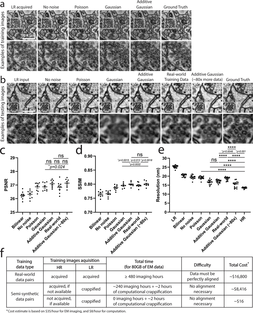
We hypothesized that to simulate real-world, low pixel resolution acquisitions with lower electron doses, our “crappifier” must add noise while also decreasing the pixel resolution. To create a suitable crappifier, we performed an ablation study, wherein we compared the performance of models trained with image pairs generated with different crappifiers, while all other factors were kept constant (Fig. 1a–e – see Methods for full details). Specifically, we compared models crappified with no noise (i.e., downsampling only), Poisson noise, Gaussian noise (independently and identically distributed), and Additive-Gaussian distributed noise, respectively. Among all models trained with crappified pairs, “Additive-Gaussian” yielded the best results. The Additive-Gaussian model also outperformed the model trained with manually acquired training pairs (“Real-world”) across all metrics. We further compared “Additive-Gaussian” with “Additive-Gaussian (~80x)”, where we used approximately 80x more training data, which interestingly did not significantly increase the Peak-Signal-to-Noise Ratio (PSNR) or Structural Similarity (SSIM) measurements, but did further increase the resolution as measured by Fourier Ring Correlation (FRC) analysis. Notably, it would have taken >480 hours of imaging time, and cost >$16,000 to acquire the same amount of real-world training data pairs as was used in our 80x Additive-Gaussian model. But by using pre-existing gold standard high-resolution data that was already acquired for separate experimental purposes, we were able to generate training data in only 2 hours, at a cost of only $16 (Fig. 1f). This highlights the utility of the crappifier method, which facilitates the generation of much larger amounts of training data at a fraction of the cost. Therefore, for our training data we “crappified” ~130GB training data of 2nm pixel transmission-mode scanning electron microscope (tSEM²⁴) images of 40nm ultrathin sections of rat CA1 hippocampal tissue. We then trained our image pairs with a ResNet-based U-Net architecture (Fig. 2a, Extended Data Fig. 1 – see Methods and Tables for full details). Using a Mean Squared Error (MSE) loss function yielded excellent results as determined by visual inspection as well as PSNR, SSIM, and FRC analyses. Overall, the PSSR-restored images from our semi-synthetic pairs contained more high-frequency information than our LR images, and yet displayed less noise than both our LR and HR images, making it easier to identify smaller objects, such as 35nm presynaptic vesicles (Fig. 2b).

Fig. 1 |. Evaluation of crappifiers with different noise injection on EM data.

a, Different crappifiers applied to high resolution, high SNR images, including “No noise” (no added noise, downsampled pixel size only), “Poisson”, “Gaussian”, and “Additive Gaussian” noise. The real-world acquired low- (LR acquired) and high-resolution (Ground Truth) images are also shown for comparison. Each training set contains 40 image pairs, achieving similar results. b, Visualized restoration performance of PSSR models that were trained on each different crappifier (No noise, Poisson, Gaussian, and Additive Gaussian), as well as a model trained with manually acquired low-resolution versions of the same samples used for the high-resolution semi-synthetic training data (“Real-world Training Data”). Results from a model that using the same crappifier as “Additive Gaussian”, but with ~80x more training data (“Additive Gaussian (~80x)”) are also displayed. LR input and Ground truth of the example testing ROI are also shown. Experiments were repeated with 8–16 images, achieving similar results. PSNR (c), SSIM (d) and resolution as measured by Fourier Ring Correlation analysis (FRC) (e) (PSNR and SSIM, n = 8 independent images; FRC resolution, n = 16 independent images). f, Shown is a table that compares the devoted time, cost and difficulty level between experiments with manually acquired training pairs and experiments using our crappification method. All values are shown as mean ± SEM. ns = not significant. P values are specified in the figure for 0.0001<p<0.05. *p<0.05, **p<0.01, ***p<0.001, ****p<0.0001, ns = not significant; Two-sided paired t-test.

Fig. 2 |. Restoration of semi-synthetic and real-world EM testing data using PSSR model trained on semi-synthetically generated training pairs.

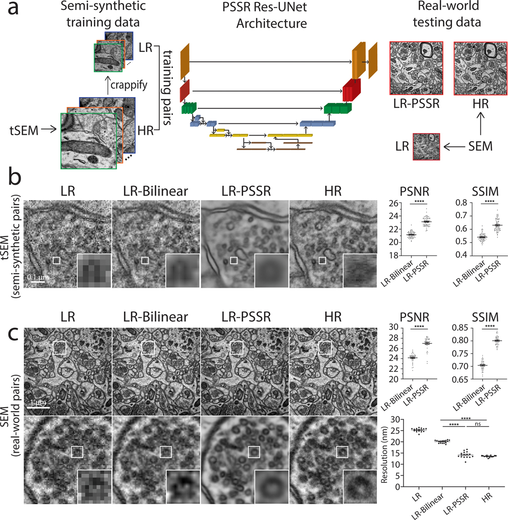
a, Overview of the general workflow. Training pairs were semi-synthetically created by applying a degrading function to the HR images taken from a scanning electron microscope in transmission mode (tSEM) to generate LR counterparts (left column). Semi-synthetic pairs were used as training data through a dynamic ResNet-based U-Net architecture. Layers of the same xy size are in the same color (middle column). Real-world LR and HR image pairs were both manually acquired under a SEM (right column). The output from PSSR (LR-PSSR) when LR is served as input is then compared to HR to evaluate the performance of our trained model. b, Restoration performance on semi-synthetic testing pairs from tSEM. Shown is the same field of view of a representative bouton region from the synthetically created LR input with the pixel size of 8nm (left column), a 16x bilinear upsampled image with 2nm pixel size (second column), 16x PSSR upsampled result with 2nm pixel size (third column) and the HR ground truth acquired at the microscope with the pixel size of 2nm (fourth column). A close view of the same vesicle in each image is highlighted. The Peak-Signal-to-Noise-Ratio (PSNR) and the Structural Similarity (SSIM) quantification of the semi-synthetic testing sets are shown (right) (n = 66 independent images). c, Restoration results of manually acquired SEM testing pairs. Shown is the comparison of the LR input acquired at the microscope with a pixel size of 8nm (left column), 16x bilinear upsampled image (second column), 16x PSSR upsampled output (third column) and the HR ground truth acquired at the microscope with a pixel size of 2nm (fourth column). Bottom row compares the enlarged region of a presynaptic bouton with one vesicle highlighted in the inset. Graphs comparing PSNR, SSIM and image resolution are also displayed (right). The PSNR and SSIM values were calculated between an upsampled result and its corresponding HR ground truth (n = 42 independent images). Resolution was calculated with the Fourier Ring Correlation (FRC) plugin in NanoJ-SQUIRREL by acquiring two independent images at low and high-resolution (n = 16 independent images). All values are shown as mean ± SEM. P values are specified in the figure for 0.0001<p<0.05. *p<0.05, **p<0.01, ***p<0.001, ****p<0.0001, ns = not significant; Two-sided paired t-test.

We next tested whether our PSSR model was effective on real-world LR acquisitions. DL-based models are notoriously sensitive to variations in training versus testing data, usually precluding the use of models generated from training images acquired in one condition on images acquired in another (i.e. data generated using a different sample preparation technique, type, or on a different microscope). Similarly, there is a risk that models trained on artificially injected noise will learn how to remove artificial noise yet fail to remove real-world noise.

Our training images were generated from 40nm sections of rat CA1 tissue acquired with a tSEM detector. But for our testing data, we acquired HR and LR images of 80nm sections of dentate gyrus tissue from a mouse brain, imaged with a backscatter detector. Based on several metrics including PSNR, SSIM, FRC (Fig. 2b–c), NanoJ-SQUIRREL error mapping analysis (Extended Data Fig. 2)²⁵, visual inspection, and comparison to the Block-Matching and 3D filtering (BM3D) denoising method (Extended Data Fig. 3)²⁶, we found PSSR successfully restored real-world LR images (Fig. 2c). Thus, our PSSR model is effective for real-world data, and is not restricted to data acquired in the exact same fashion as the training set.

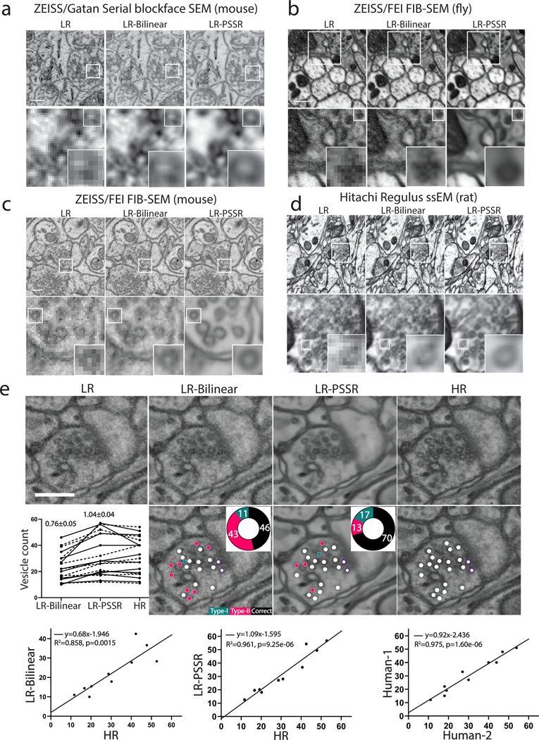
We next asked whether we could sufficiently restore 8nm SBFSEM datasets to 2nm using PSSR, since high quality 2nm SBFSEM imaging is currently difficult or impossible for us to achieve. Using the same PSSR model described above we were able to restore an 8nm pixel SBFSEM 3D dataset to 2nm (Fig. 3a, Supplementary Video 2). Remarkably, our PSSR model also worked very well on mouse, rat, and fly samples imaged on four different microscopes in four different labs (Fig. 3a–d). In addition to our SBFSEM and SEM imaging systems, PSSR processing appeared to restore images acquired on a ZEISS FIB-SEM (from the Hess lab at Janelia Farms, Fig. 3c, Supplementary Video 3) and a Hitachi Regulus FE-SEM (from the Kubota lab at National Institute for Physiological Sciences, Fig. 3d). PSSR processing also performed well on a 10×10×10nm resolution FIB-SEM fly brain dataset, resulting in a 2×2×10nm resolution dataset with higher SNR and resolution (Fig. 3b). Thus, PSSR can provide 25x super-resolution with useful results, effectively increasing the lateral resolution and speed of FIB-SEM imaging by a factor of at least 25x.

Fig. 3 |. PSSR model is effective for multiple EM modalities and sample types.

Shown are representative low-resolution (LR), bilinear interpolated (LR-Bilinear) and PSSR-restored (LR-PSSR) images from mouse brain sections (n = 75 sections in one image stack, xy dimension 240×240 pixels) imaged with a ZEISS Sigma-VP Gatan Serial Blockface SEM system (a), fly sections (n = 50 sections in one image stack, xy dimension 1250×1250 pixels) acquired with ZEISS/FEI focused ion beam-SEM (FIB-SEM) (b), mouse sections (n = 563 sections in one image stack, xy dimension 240×240 pixels) from ZEISS/FEI FIB-SEM (c) and rat sections (one montage, xy dimension 2048×1024 pixels) imaged with a Hitachi Regulus serial section EM (ssEM) (d). e, Validation of pre-synaptic vesicle detection. LR, LR-Bilinear, LR-PSSR, and ground truth high-resolution (HR) images of a representative bouton region as well as their color-labeled vesicle counts are shown. Vesicles colored with red represents false negatives, blue are false positives, and white are true positives. The percentage of each error type is shown in the pie chart. Docked vesicles were labelled with purple dots. Vesicle counts from two humans were plotted (Dashed line: Human-1, solid line: Human-2), with the average total error ± SEM. displayed above. Experiments were conducted with n=10 independent bouton regions in all conditions, achieving similar results. The linear regression between LR-Bilinear and HR, LR-PSSR and HR, and two human counters of HR are shown in the third row. The equation for the linear regression, the Goodness-of-Fit (R²) and the p-value (p) of each graph are displayed. Scale bars = 1.5μm.

The major concern with DL-based image processing is the possibility of false positives (aka “hallucinations”)^5,9,27,28. To further test the accuracy and utility of the PSSR output within a more concrete, biological context, we next randomized LR-Bilinear, LR-PSSR, and HR images, then distributed them to two blinded human experts for manual segmentation of presynaptic vesicles, which are difficult to detect with 8nm pixel resolution images (see Supplementary Notes and Methods for full details). We found the LR-PSSR segmentation was significantly more accurate than the LR-Bilinear (Fig. 3e). Interestingly, while the LR-PSSR output significantly reduced false negatives, the LR-PSSR output had a slightly higher number of “false positives” than the LR-Bilinear. However, the variance between the LR-PSSR and HR results was similar to the variance between the two expert human results on HR data (Fig. 3e), which is the current gold standard. Notably, we found PSSR images were much easier to segment - a major bottleneck for analyzing 3DEM datasets (Supplementary Video 4).

Similar to SBFSEM, laser scanning confocal microscopy also suffers from a direct relationship between pixel resolution and sample damage (i.e. phototoxicity/photobleaching)²⁹. This can be a major barrier for cell biologists who wish to study the dynamics of smaller structures such as mitochondria, which regularly undergo fission and fusion, but also show increased fission and swelling in response to phototoxicity (Supplementary Video 5, Extended Data Fig. 4).

Laser scanning microscopy also suffers from an inverse relationship between pixel resolution and imaging speed, making live cell imaging of faster processes (e.g. organelle motility in neurons) challenging if not impossible. Nonetheless, Nyquist sampling criteria often necessitates the use of smaller pixels to resolve smaller structures – this is particularly true for higher resolution imaging methods that depend on post-processing pixel reassignment and/or deconvolution. Thus, we sought to determine whether PSSR might enable acquisitions with decreased pixel resolution in order to optimize the imaging speed and SNR of live laser scanning confocal microscope imaging. Importantly, to train a DL model using image pairs of mitochondria in live cells is virtually impossible because they are constantly moving and changing their shape. Thus, our “crappification” approach is particularly useful generating training data for live cell imaging datasets.

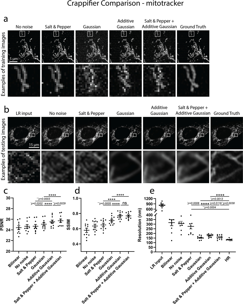
To generate our ground truth training dataset we used a ZEISS LSM 880 in Airyscan mode (see Online Methods for more details). Similar to our EM model, an ablation study that compared crappifiers with different noise distributions was conducted (Extended Data Fig. 5 – See Methods for full details). We found the crappifier injected with Salt & Pepper and Additive-Gaussian noise yielded overall best performance. For the real-world LR test data, we acquired images in confocal mode at 16x lower pixel resolution with a 2.5 AU pinhole on a PMT confocal detector, without any additional image processing. To ensure minimal phototoxicity, we also decreased the laser power for our LR acquisitions by a factor of 4 or 5 (see Tables 1–2 for more details), resulting in a net laser dose decrease of ~64–80x. Thus, our PSSR model was trained to restore low-resolution, low SNR, low pixel resolution confocal images to high SNR, high pixel resolution, high “optical” (i.e. deblurred) resolution Airyscan-equivalent image quality. To start, we trained on live cell timelapse acquisitions of mitochondria in U2OS cells. As expected, imaging at full resolution resulted in significant bleaching and phototoxicity-induced mitochondrial swelling and fission (Supplementary Video 5). However, the LR acquisitions were extremely noisy and pixelated due to undersampling. However, the LR scans showed far less photobleaching (Extended Data Fig. 4). Similar to our EM data, LR-PSSR images had higher SNR and resolution compared to LR acquisitions, as determined by testing on both semi-synthetic and real-world low- versus high-resolution image pairs. Notably, LR-PSSR images also had higher SNR than HR images (Fig. 4d).

Table 1:

Details of fluorescence PSSR training experiments.

Experiment	U2OS MitoTracker PSSR-SF	U2OS MitoTracker PSSR-MF	Neuron Mito-dsRed PSSR-MF
Input size (x, y, z)	(128, 128, 1)	(128, 128, 5)	(128, 128, 5)
Output size (x, y, z)	(512, 512, 1)	(512, 512, 1)	(512, 512, 1)
No. of image pairs for training	5000	5000	3000
No. of image pairs for validation	200	200	300
No. of GPUs	2	2	2
Training datasource size (GB)	9.4	9.4	9.5
Validation datasource size (GB)	0.44	0.44	1.8
Training dataset size (GB)	1.38	1.7	1.03
Validation dataset size (GB)	0.06	0.07	0.1
Batch size per GPU	8	8	6
No. of epochs	100	100	50
Training time (h)	3.76	3.77	1.25
Learning rate	4e-4	4e-4	4e-4
Best model found at epoch	33	86	39
Normalized to ImageNet statistics?	No	No	No
ResNet size	ResNet34	ResNet34	ResNet34
Loss function	MSE	MSE	MSE

Table 2:

Details of fluorescence PSSR testing data for PSNR, SSIM, and error-mapping.

	U2OS MitoTracker			Neuron Mito-dsRed
	Semi-synthetic	Real-world		Semi-synthetic	Real-world
	HR	LR	HR	HR	LR	HR
Microscopy	Airyscan	Confocal	Airyscan	Airyscan	Confocal	Airyscan
Laser power (μW)	35	7	28	82	11	55
Data source size (MB)	1250	7.15	200	5920	10.7	305
Data set size (MB)	325	6.39	191	1970	10.4	305
Total number of different cells	6	10	10	7	10	10

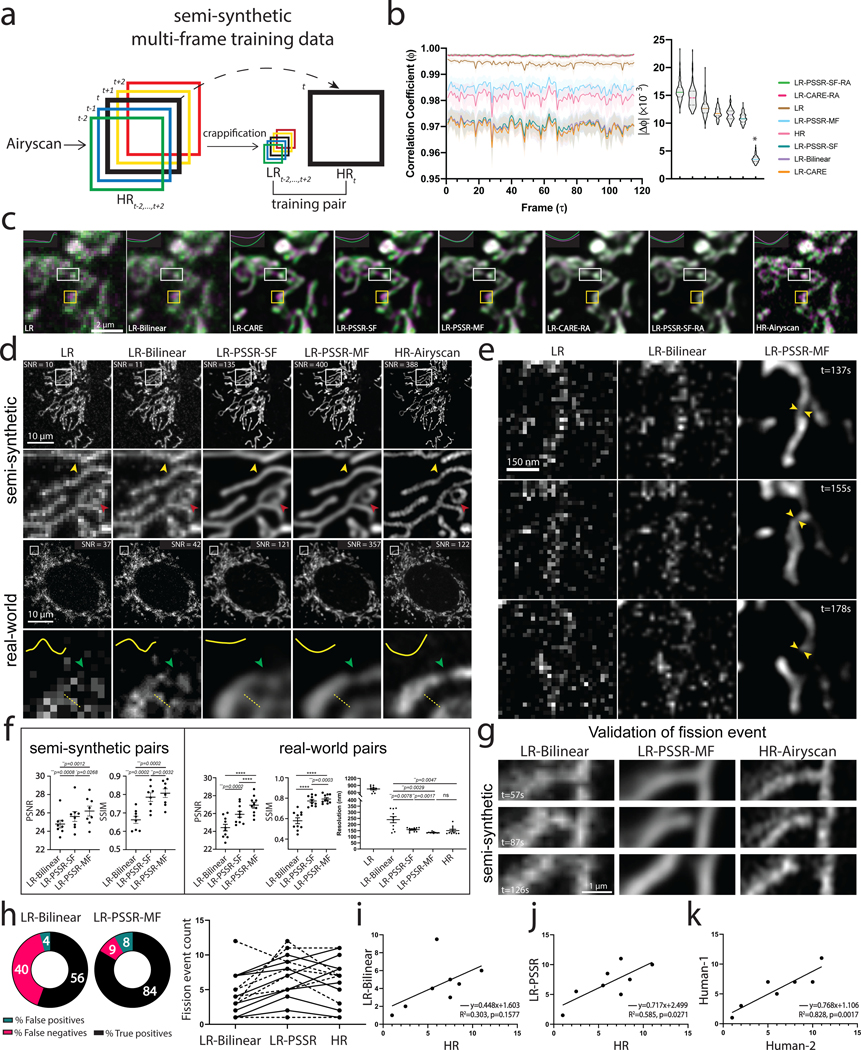
Fig. 4 |. Multi-frame PSSR timelapses of mitochondrial dynamics.

a, Overview of multi-frame PSSR training data generation method. Five consecutive frames (${HR}_i, i\in \left[t-2, t+2\right]$) from a HR Airyscan time-lapse movie were synthetically crappified to five LR images (${LR}_i, i\in \left[t-2, t+2\right]$), which together with the HR middle frame at time $t \left({HR}_t\right)$, form a five-to-one training “pair”. b, Temporal consistency analysis. Neighboring-frame cross-correlation coefficient ($\varnothing (X_{\tau }, X_{\tau +1}))$ that corresponds to frame $\tau$ in $x$-axis denotes the correlation coefficient of frame $\tau (X_{\tau }$) and frame $\tau +1\left(X_{\tau +1}\right)$ (Left). Absolute error against HR ($\left|∆\varnothing \right|$) for each condition was compared ($\left|∆\varnothing \right|=\left|{\varnothing }_{\tau }-{\varnothing }_{\tau }^{HR}\right|$, right). n = 6 independent timelapses with n = 80–120 timepoints each. Colored shades show standard error. The * sign above LR-PSSR-MF denotes that LR-PSSR-MF is significantly more consistent with HR than all other conditions (P<0.0001). All violin plots show lines at the median and quartiles. c, Examples of false mitochondrial network merges (white boxes) due to the severe flickering artifacts in single-frame models (LR-Bilinear, LR-CARE and LR-PSSR-SF), and loss of temporal consistency and resolution (yellow boxes) in models post-processed with a “rolling frame averaging” method (LR-CARE-RA and LR-PSSR-SF-RA). Two consecutive frames of an example region from semi-synthetic acquired low-resolution (LR), bilinearly upsampled (LR-Bilinear), CARE (LR-CARE), 5-frame Rolling Average post-processed CARE output (LR-CARE-RA), single-frame PSSR (LR-PSSR-SF), single-frame PSSR post-processed with a 5-frame Rolling Average (LR-PSSR-RA), 5-frame multi-frame PSSR (LR-PSSR-MF), and ground truth high-resolution (HR-Airyscan) time-lapses are color coded in magenta ($t=0s$) and green ($t=5s$). Insets show the intensity line plot of the two frames drawn in the center of the white box in each condition. The yellow box shows an example of temporal resolution loss in RA conditions (LR-CARE-RA and LR-PSSR-SF-RA) only. Magenta pixels represent signal that only exists in the t=0s frame, but not in the t=5s, while green pixels represent signal present only in the t=5s frame. d, Restoration performance on semi-synthetic and real-world testing pairs. For the semi-synthetic pair, LR was synthetically generated from Airyscan HR movies. Enlarged ROIs show an example of well resolved mitochondrial structures by PSSR, agreeing with Airyscan ground truth images. Red and yellow arrowheads show two false connecting points in LR-Bilinear and LR-PSSR-SF, which were well separated in LR-PSSR-MF. In the real-world example, green arrowheads in the enlarged ROIs highlight a well restored gap between two mitochondria segments in the LR-PSSR-MF output. Normalized line-plot cross-section profile (yellow) highlights false bridging between two neighboring structures in LR-Bilinear and LR-PSSR-SF, which was well separated with our PSSR-MF model. Signal-to-Noise Ratio (SNR) measured using the images in both semi-synthetic and real-world examples are indicated. e, PSSR output captured a transient mitochondrial fission event. Shown is a PSSR-restored dynamic mitochondrial fission event, with three key time frames displayed. Arrows highlight the mitochondrial fission site. f, PSNR and SSIM quantification of the semi-synthetic (n = 8 independent timelapses with n = 80–120 timepoints each) as well as the real-world (n = 10 independent timelapses of fixed samples with n=10 timepoints each) testing sets discussed in (d). FRC values measured using two independent low- versus high- resolution acquisitions from multiple cells are indicated (n = 10). g, Validation of fission event captures using semi-synthetic data. An example of a fission event that was detectable in LR-PSSR but not LR-Bilinear. Experiments were repeated with 8 timelapses, achieving similar results. h, For fission event detection, the number of false positives, false negatives, and true positives detected by expert humans was quantified for 8 different timelapses. Distribution was shown in the pie charts. Fission event counts from two humans were plotted (Dashed line: Human-1, solid line: Human-2). i-k, Linear regression between LR-Bilinear and HR, LR-PSSR and HR, and two human counters of HR are shown (n = 8 independent timelapses with n = 80–120 timepoints each). The linear regression equation, the Goodness-of-Fit (R²) and the p-value of each graph are displayed. All values are shown as mean ± SEM. P values are specified in the figure for 0.0001<p<0.05. *p<0.05, **p<0.01, ***p<0.001, ****p<0.0001, ns = not significant; Two-sided paired t-test.

We observed significant “flickering” in LR-PSSR timelapses (Supplementary Video 6, Figure 4b) due to noise-induced variations in signal detection and image reconstruction, causing both false breaks and merges in mitochondrial networks (Fig. 4c, white boxes, Fig. 4d, red and yellow arrows), making it impossible to accurately detect bona fide mitochondrial fission or fusion events. This temporal inconsistency was reflected in neighboring-frame cross-correlation analysis (Fig. 4b, see Methods for full details). One strategy for increasing the SNR of images is to average multiple scans, e.g. “frame averaging” – this method can also be used to reduce “flickering” effects in videos (Fig. 4b). However, this approach is problematic for live imaging of quickly moving objects: If objects move greater than half the distance of the desired spatial resolution between individual frames, temporal Nyquist criteria are no longer satisfied, resulting in blurring artifacts and loss of both spatial and temporal resolution^30,31. This loss of information is compounded if spatial Nyquist criteria are also unmet, i.e. when subsampling pixels, as is the case in LR acquisitions. However, although simple frame averaging approaches may lose resolution in exchange for higher SNR, more sophisticated computational approaches can take advantage of multi-frame acquisitions to increase the resolution of individual frame reconstructions^32–35.

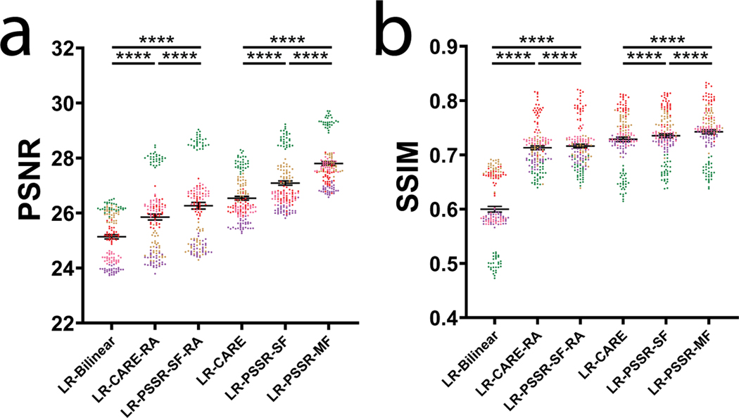
We hypothesized that the PSSR network could learn the additional information contained in sequential video frames, even when grossly undersampled in both space and time, and could thus be used to reduce flickering artifacts, while also improving the restoration accuracy and resolution of PSSR-processed timelapse videos. To test this hypothesis, we exploited the multi-dimensional capabilities of our PSSR Res-UNet architecture by training on 5 sequential timepoint inputs for each single timepoint output (multi-frame PSSR, or “PSSR-MF”, Fig. 4a). As measured by PSNR, SSIM, FRC, and NanoJ-SQUIRREL error mapping, as well as compared with the BM3D denoising algorithm, PSSR-MF processing of LR acquisitions (LR-PSSR-MF) showed significantly increased resolution and SNR compared to the raw input (LR), 16x bilinear interpolated input (LR-Bilinear), and single-frame PSSR (LR-PSSR-SF) (Fig. 4d, 4f, Extended Data Fig. 7–8). Since it is conceivable that simply averaging 5 frames would yield similar improvements due to reduced flickering and increased SNR, we tested whether using a 5-frame rolling average over the LR-PSSR-SF output (LR-PSSR-SF-RA) could yield similar results to LR-PSSR-MF. Although LR-PSSR-SF-RA output displayed reduced flickering (Fig. 4b–c), we found that LR-PSSR-SF-RA performed significantly worse than LR-PSSR-MF in terms of both resolution and accuracy (Fig. 4c, Extended Data Fig. 6, Supplementary Video 6). We also compared PSSR models with Content-Aware Image Restoration (CARE), a gold-standard DL-based image restoration algorithm (Fig. 4b–c, Extended Data Fig. 6 – see Methods for full details). Specifically, CARE trained results (LR-CARE) and its Rolling Average post-processed version (LR-CARE-RA) were compared with multi-frame PSSR (LR-PSSR-MF), singe-frame PSSR (LR-PSSR-SF) and its Rolling Average post-processed results (LR-PSSR-SF-RA). As expected, the LR-CARE and LR-PSSR-SF results were similar. However, we found the multi-frame PSSR approach yielded better results than CARE, both before and after the Rolling Average processing (Extended Data Fig. 6). We therefore concluded multi-frame PSSR significantly enhances the fidelity and resolution of LR images beyond any standard frame-by-frame image restoration approach.

For all time-lapse PSSR we used PSSR-MF and refer to it as PSSR for the remainder of this article. The improved speed, resolution, and SNR enabled us to detect mitochondrial fission events that were not detectable in the LR or LR-Bilinear images (yellow arrows, Fig. 4e, Supplementary Video 7). Additionally, the relatively high laser dose during HR acquisitions raises questions as to whether observed fission events are artifacts of phototoxicity. We validated the accuracy of our fission event detection with semi-synthetic data quantified by two expert humans (Fig. 4g–h). We found a significant improvement in detecting fission events with relatively minor increases in false positives (Fig. 4h–k). We again found the variance between the PSSR and HR results was similar to the variance between the two expert human results on HR data. Thus, our PSSR model provides an opportunity to detect very fast mitochondrial fission events with fewer phototoxicity-induced artifacts than standard high-resolution Airyscan imaging using normal confocal optics and detectors.

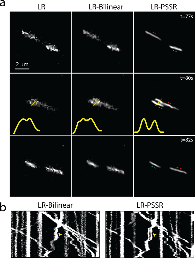
As mentioned above, in addition to phototoxicity issues, the slow speed of HR scanning confocal imaging often results in temporal undersampling of fast-moving structures such as motile mitochondria in neurons (Supplementary Fig. 1, Supplementary Videos 8–9). However, relatively fast LR scans do not provide sufficient pixel resolution or SNR to resolve fission or fusion events, or individual mitochondria when they pass one another along a neuronal process, which can result in faulty analysis or data interpretation (Supplementary Video 8). Thus, we next tested whether PSSR provided sufficient restoration of undersampled time-lapse imaging of mitochondrial trafficking in neurons.

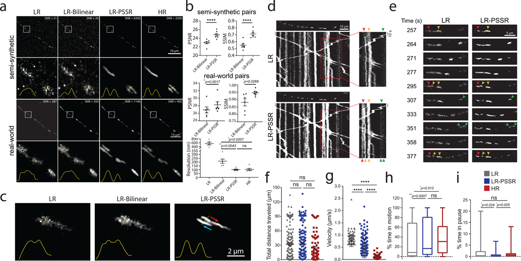
As measured by PSNR, SSIM, FRC, and NanoJ-SQUIRREL error mapping, the overall resolution and SNR improvement provided by PSSR enabled us to resolve adjacent mitochondria as well as fission and fusion events (Fig. 5a–c, Extended Data Fig. 9–10, Supplementary Video 9). Since our LR acquisition rates are 16x faster than HR, instantaneous motility details were preserved in LR-PSSR whereas in HR images they were lost (Fig. 5d, Supplementary Fig. 1, Supplementary Video 9). The overall total distance mitochondria travelled in neuronal processes was the same for both LR and HR (Fig. 5f). However, we were able to obtain unique information about how they translocate when imaging at a 16x higher frame rate (Fig. 5g). Interestingly, a larger range of velocities was identified in LR-PSSR than both LR and HR images. Overall, LR-PSSR and HR provided similar values for the percent time mitochondria spent in motion (Fig. 5h). Smaller distances travelled were easier to detect in our LR-PSSR images, and therefore there was an overall reduction in the percent time mitochondria spent in the paused position in our LR-PSSR data (Fig. 5i). Taken together, these data show PSSR provides a means to detect critical biological events that would not be possible with conventional HR or LR imaging.

Fig. 5 |. Spatiotemporal analysis of mitochondrial motility in neurons.

PSSR facilitates high spatiotemporal resolution imaging of mitochondrial motility in neurons. a, Comparison of PSSR results (LR-PSSR) versus bilinear interpolation (LR-Bilinear) on semi-synthetic (n = 7 independent timelapse movies with n=100 independent time points each) and real-world testing pairs (n = 6 independent timelapse movies with n=12 independent time points each). Enlarged ROIs from representative images show PSSR resolved two mitochondria in both semi-synthetic and real-world testing sets, quantified by normalized line plot cross-section profiles. SNR b, PSNR (top) and SSIM (middle) quantification of the datasets in (a). FRC resolution measured from two independent acquisitions of the real-world overview dataset discussed in (a) is indicated (bottom). c, PSSR restoration of LR timelapses resolves mitochondria moving past one another in a neuronal process (arrows indicate direction of movement). d, Representative kymographs of mitochondrial motility in hippocampal neurons transfected with Mito-DsRed (n = 7 independent LR timelapse movies processed to LR-PSSR). First frame of each time-lapse movie is shown above each kymograph. Different color arrowheads indicate mitochondria going through fission and fusion events. Each color represents a different mitochondrion. e, Enlarged areas of (d), capturing mitochondrial fission and fusion events in real-time. f-i, Mitochondrial motility was quantified from time-lapse movies as demonstrated in Supplementary Video 8. For each mitochondrial trajectory the total distance mitochondria travelled (f), mitochondrial velocity (g), percent time mitochondria spent in motion (h) and in pause (i) was quantified (n = 76 – 216 mitochondria from 4 neurons and 3 independent experiments). All values are shown as mean ± SEM. P values are specified in the figure for 0.0001<p<0.05. *p<0.05, **p<0.01, ***p<0.001, ****p<0.0001, ns = not significant; Two-sided paired t-test (b) and Kruskal-Wallis test followed by Dunn’s multiple comparison test (f-i).

Discussion

We have demonstrated DL-based pixel super-resolution can be a viable strategy of particular value for both optical and electron point-scanning microscopes. Acquiring suitably aligned pairs of high- and low-quality images for training is incredibly expensive and difficult (Fig. 1f). Thus, we introduced a novel “crappifier” for generating noisy, low-resolution training data from high-resolution, high SNR ground truth data. This enables the use of large, pre-existing gold standard datasets for training new models without acquiring any new data. We hope the open-source availability of our crappifier will be reciprocated by open-source sharing of high-quality imaging data, which can then be used to train new DL models. We did not fully explore all possibilities for a crappifier and believe this is an open and fruitful area for future studies.

We discovered that DL-based restoration of noisy timelapses suffers from temporal inconsistency (“flickering”) artifacts due to noise-induced randomness in pixel values between frames. To address this, we introduced a multi-frame super-resolution approach that leverages the information in previous and future timepoints to better infer the frame of interest. We found this multi-frame approach not only reduces flickering artifacts, but also provides better overall image restoration for each independent frame. Notably, this approach would be impossible without the crappifier, which provides the ability to generate training data from videos of rapidly moving structures in live cells for which it is impossible to acquire perfectly aligned image pairs.

Any output from a DL super-resolution model is a prediction, is never 100% accurate, and is always highly dependent on sufficient correspondence between the training versus experimental data^5,9,28,36. Whether the level of accuracy of a given model for a given dataset is satisfactory is ultimately dependent on the tolerance for error in the measurement being made. For example, our EM PSSR model was validated by segmenting vesicles in presynaptic boutons. But we did not rule out the possibility that other structures or regions in the same sample may not be restored by our model with the necessary accuracy for any arbitrary measurement. Thus, it is essential to validate the accuracy of the model for the specific task at hand before investing further. Similarly, we observed that no single performance metric reliably captures the “best” model. Thus, model performance must be evaluated by a combination of metrics, segmentation, and, of course, visual inspection by human experts. An important future direction may be to develop better metrics for evaluating models.

Though the accuracy of DL approaches such as PSSR is technically imperfect, real-world limitations on acquiring ground truth data may render PSSR the best option. Our results show the PSSR approach can in principle enable higher speed and resolution imaging with the fidelity necessary for biological research. The ability to use DL to supersample undersampled images provides an opportunity that extends to any point-scanning system, including ion-based imaging systems^37,38 or high-resolution cryoSTEM³⁹.

For future uses of PSSR, we propose an acquisition scheme wherein a relatively limited number of “ground truth” HR images are acquired for fine-tuning pre-trained models. More importantly, the performance of generalized, unsupervised or “self-supervised” denoising approaches^7,10 as well as DL-enabled deconvolution approaches^19,20 suggests we may one day be able to generate a more generalized model for a specific imaging system, instead of a specific sample type.

Structured illumination microscopy, single-molecule localization microscopy, and pixel reassignment microscopy demonstrate the power of configuring optical imaging schemes with a specific post-processing computational strategy in mind. The power of deep convolutional neural networks for post-processing image data presents a new opportunity for redesigning imaging systems to exploit these capabilities to minimize costs traditionally considered necessary for extracting meaningful imaging data. Similarly, automated real-time corrections to the images and real-time feedback to the imaging hardware are now within reach. This is an exciting area of active investigation in our laboratory and others (Lu Mi, Yaron Meirovitch, Jeff Lichtman, Aravinthan Samuel, Nir Shavit, personal communication).

Online Methods

Semi-synthetic Training Image Generation

HR images were acquired using scanning electron or Airyscan confocal microscopes. Due to the variance of image properties (e.g. format, size, dynamic range and depth) in the acquired HR images, data cleaning is indispensable for generating training sets that can be easily accessed during training. In this article, we differentiate the concept of “data sources” and “data sets”, where data sources refer to uncleaned acquired high-resolution images, while data sets refer to images that are generated and preprocessed from data sources. HR data sets were obtained after preprocessing HR images from data sources, LR data sets were generated from HR data sets using a “crappifier” function.

Preprocessing.

Tiles of predefined sizes (e.g. 256 × 256 and 512 × 512 pixels) were randomly cropped from each frame in image stacks from HR data sources. “Refection padding” was used if the image size in the data sources is smaller than the predefined tile size. All tiles were saved as separate images in .tif format, which together formed a HR data set.

Image Crappification.

A “crappifier” was then used to synthetically degrade the HR data sets to LR images, with the goal of approximating the undesired and unavoidable pixel intensity variation in real-world low-resolution and low SNR images of the same field of view directly taken under an imaging system. These HR images together with their corrupted counterparts served as training pairs to facilitate “deCrappification”. The crappification function can be simple, but it materially improves both the quality and characteristics of PSSR outputs.

Image sets were normalized from 0 to 1 before being 16x downsampled in pixel resolution (e.g. a 1000 × 1000 pixel image would be downsampled to 250 × 250 pixels). To mimic the image quality degradation caused by 16x undersampling on a real-world point-scanning imaging system, salt-and-pepper noise, and Gaussian additive noise with specified local variance were randomly injected into the high-resolution images. The degraded images were then rescaled to 8-bit for viewing with normal image analysis software.

EM Crappifier

Random Gaussian-distributed additive noise (${\mu }_{EM}=0,\mathrm{ }{\sigma }_{EM}=3$) was injected. The degraded images were then downsampled using spline interpolation of order 1.

MitoTracker and Neuronal Mitochondria Crappifier

The crappification of MitoTracker and neuronal mitochondria data followed a similar procedure. Salt-and-pepper noise was randomly injected in 0.5% of each image’s pixels replacing them with noise, which was followed by the injection of random Gaussian-distributed additive noise (${\mu }_{LSM}=0,\mathrm{ }{\sigma }_{LSM}=5$). The crappified images were then downsampled using spline interpolation of order 1.

Data Augmentation.

After crappified low-resolution images were generated, we used data augmentation techniques such as random cropping, dihedral affine function, rotation, random zoom to increase the variety and size of our training data⁴⁰.

Multi-frame Training Pairs.

Unlike imaging data of fixed samples, where we use traditional one-to-one high- and low-resolution images as training pairs, for time-lapse movies, five consecutive frames (${HR}_i,\mathrm{ }i\in \left[t-2,\mathrm{ }t+2\right]$) from a HR Airyscan time-lapse movie were synthetically crappified to five LR images (${LR}_i,\mathrm{ }i\in \left[t-2,\mathrm{ }t+2\right]$), which together with the HR middle frame at time $t\mathrm{ }\left({HR}_t\right)$, form a five-to-one training “pair”. The design of five-to-one training “pairs” leverages the spatiotemporal continuity of dynamic biological behaviors. (Fig. 4a).

Crappifier comparison

EM crappifier comparison.

Four crappifiers including “No noise”, “Poisson”, “Gaussian” and “Additive Gaussian” were used to generate semi-synthetic training pairs from the same set of HR SEM images. The “No noise” crappifier simply downsampled HR image pixel sizes by a factor of 16x (4×4) without adding any noise, while the “Poisson”, “Gaussian” and “Additive Gaussian” crappifiers added random Poisson noise, random Gaussian noise (${\mu }_{EM}=0,\mathrm{ }{\sigma }_{EM}=0.15$) and random Gaussian-distributed additive noise (${\mu }_{EM}=0,\mathrm{ }{\sigma }_{EM}=3$) respectively, before applying pixel downsampling. “Additive Gaussian (~80x)” used the same crappifier as “Additive Gaussian”, but with ~80x more training data. We also compared the models described above with “Real-world”, a model trained with real-world pairs, whose HR images are the same as the HR images of the semi-synthetically generated training pairs, but whose LR images were manually acquired at the microscope.

MitoTracker crappifier comparison.

Five crappifiers including “No noise”, “Salt & Pepper”, “Gaussian”, “Additive Gaussian” and “Salt & Pepper + Additive Gaussian” were used to generate semi-synthetic training pairs from the same set of HR Airyscan MitoTracker time-lapse videos. The “No noise” crappifier downsampled HR image pixel sizes by a factor of 16x (4×4) without adding any noise, while the “Salt & Pepper”, “Gaussian”, “Additive Gaussian”, and “Salt & Pepper + Additive Gaussian” crappifiers added random Salt & Pepper noise (0.5%), random Gaussian noise (${\mu }_{LSM}=0,\mathrm{ }{\sigma }_{LSM}=0.025$), random Gaussian-distributed additive noise (${\mu }_{LSM}=0,\mathrm{ }{\sigma }_{LSM}=5$), and the combination of “Salt & Pepper” and “Additive Gaussian” respectively, before the bilinear downsampling.

Neural Networks

Single-frame Neural Network (PSSR-SF).

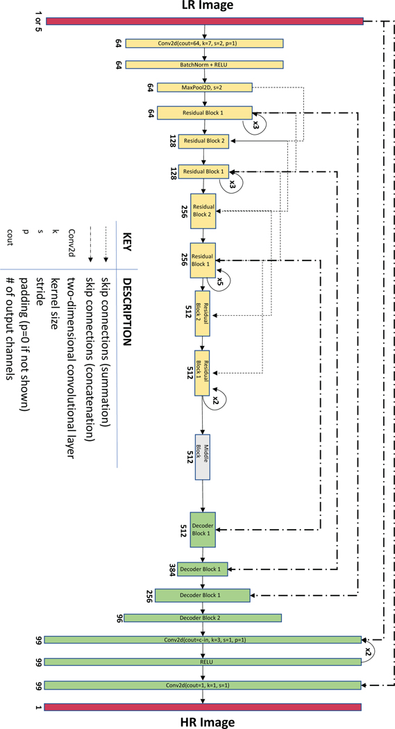
A ResNet-based U-Net was used as our convolutional neural network for training⁴¹. Our U-Net is in the form of encoder-decoder with skip-connections, where the encoder gradually downsizes an input image, followed by the decoder upsampling the image back to its original size. For the EM data, we utilized ResNet pretrained on ImageNet as the encoder. For the design of the decoder, the traditional handcrafted bicubic upscaling filters are replaced with learnable sub-pixel convolutional layers⁴², which can be trained specifically for upsampling each feature map optimized in low-resolution parameter space. This upsampling layer design enables better performance and largely reduces computational complexity, but at the same time causes unignorable checkerboard artifacts due to the periodic time-variant property of multirate upsampling filters⁴³. A blurring technique⁴⁴ and a weight initialization method known as “sub-pixel convolution initialized to convolution neural network resize (ICNR)”⁴⁵ designed for the sub-pixel convolution upsampling layers were implemented to remove checkerboard artifacts. In detail, the blurring approach introduces an interpolation kernel of the zero-order hold with the scaling factor after each upsampling layer, the output of which gives out a non-periodic steady-state value, which satisfies a critical condition ensuring a checkerboard artifact-free upsampling scheme⁴⁴. Compared to random initialization, in addition to the benefit of removing checkerboard artifacts, ICNR also empowers the model with higher modeling power and higher accuracy⁴⁵. A self-attention layer inspired by Zhang et al.⁴⁶ was added after each convolutional layer.

Multi-frame Neural Network (PSSR-MF).

A similar yet slightly modified U-Net was used for time-lapse movie training. The input layer was redesigned to take five frames simultaneously while the last layer still produced one frame as output.

Training Details

Loss Function.

MSE loss was used as our loss function.

Optimization Methods.

Stochastic gradient descent with restarts (SGDR)⁴⁷ was implemented. Aside from the benefits we are able to get through classic stochastic gradient descent, SGDR resets the learning rate to its initial value at the beginning of each training epoch and allows it to decrease again following the shape of a cosine function, yielding lower loss with higher computational efficiency.

Cyclic Learning Rate and Momentum.

Instead of having a gradually decreasing learning rate as the training converges, we adopted cyclic learning rates⁴⁸, cycling between upper bound and lower bound, which helps oscillate towards a higher learning rate, thus avoiding saddle points in the hyper-dimensional training loss space. In addition, we followed The One Cycle Policy⁴⁹, which restricts the learning rate to only oscillate once between the upper and lower bounds. Specifically, the learning rate linearly increases from the lower bound to the upper bound as the momentum decreases from its upper bound to the lower bound linearly. In the second half of the cycle, the learning rate fits a cosine annealing decreasing from the upper bound to zero while the momentum increases from its lower bound to the upper bound following the same annealing. This training technique achieves superior regularization by preventing the network from overfitting during the middle of the learning process, as well as enables super-convergence⁵⁰ by allowing large learning rates and adaptive momentum.

Progressive Resizing (used for EM data only).

Progressive resizing was applied during the training of the EM model. Training was executed in two rounds with HR images scaled to xy pixel sizes of 256 × 256 and 512 × 512 and LR images scaled to 64 × 64 and 128 × 128 progressively. The first round was initiated with an ImageNet pretrained ResU-Net, and the model trained from the first round served as the pre-trained model for the second round. The intuition behind this is it quickly reduces the training loss by allowing the model to see lots of images at a small scale during the early stages of training. As the training progresses, the model focuses more on picking up high-frequency features reflected through fine details that are only stored within larger scale images. Therefore, features that are scale-variant can be recognized through the progressively resized learning at each scale.

Discriminative Learning Rates (used for EM data only).

To better preserve the previously learned information, discriminative learning was applied during each round of training for the purpose of fine-tuning. At the first stage of training, only the parameters from the last layer were trainable after loading a pretrained model, which either came from a large-scaled trained publicly available model (i.e., pretrained ImageNet), or from the previous round of training. The learning rate for this stage ${lr}_1$ was fixed. Parameters from all layers were set as learnable in the second stage. A linearly spaced learning rate range ${lr}_2$ was applied. The learning rate gradually increased across the layers of the entire network architecture. The number of training epochs at each round is noted as $[N_1, { N}_2]$, where $N_1$ and $N_2$ denote the epoch number used at stage one and stage two separately (Table 3).

Table 3:

Details of the EM PSSR training experiment.

EM training data
Round of progressive resizing	1	2	3
Input size $(x,\mathrm{ }\mathrm{ }y,\mathrm{ }\mathrm{ }z)$	(32, 32, 3)	(64, 64, 3)	(128, 128, 3)
Output size $(x,\mathrm{ }\mathrm{ }y,\mathrm{ }\mathrm{ }z)$	(128,128,3)	(256, 256, 3)	(512, 512, 3)
Batch size per GPU	64	16	8
No. of epochs $[N_1,\mathrm{ }{\mathrm{ }N}_2]$	[1,1]	[3,3]	[3,3]
Learning rate$\mathrm{ }[{lr}_1,\mathrm{ }{\mathrm{ }lr}_2]$	[1e-3, (1e-5,1e-3)]	[1e-3, (1e-5,1e-3)]	[1e-3, (1e-5,1e-4)]
Training dataset size (GB)	3.9	15.56	62.24
Validation dataset size (GB)	0.96	3.89	15.56
Training datasource size (GB)	105
Validation datasource size (GB)	26
No. of image pairs for training	80,000
No. of image pairs for validation	20,000
Total training time (h)	16
Normalized to ImageNet statistics?	Yes
ResNet size	ResNet34
Loss function	MSE
No. of GPUs	2

Best Model Preservation (used for fluorescence data only).

Instead of saving the last model after training a fixed number of epochs, at the end of each training epoch, PSSR checks if the validation loss goes down compared to the loss from the previous epoch and will only update the best model when a lower loss is found. This technique ensures the best model will not be missed due to local loss fluctuation during the training.

Elimination of Tiling Artifacts.

Testing images often need to be cropped into smaller tiles before being fed into our model due to the memory limit of graphic cards. This creates tiling edge artifacts around the edges of tiles when stitching them back to the original images. A Gaussian blur kernel (${\mu }_{tile}=0,\mathrm{ }{\sigma }_{tile}=1$) was applied to a 10-pixel wide rectangle region centered in each tiling edge to eliminate the artifacts.

Technical specifications.

Final models were generated using fast.ai v1.0.55 library (https://github.com/fastai/fastai), PyTorch on two NVIDIA TITAN RTX GPUs. Initial experiments were conducted using NVIDIA Tesla V100s, NVIDIA Quadro P6000s, NVIDIA Quadro M5000s, NVIDIA Titan Vs, NVIDIA GeForce GTX 1080s, or NVIDIA GeForce RTX 2080Ti GPUs.

Evaluation Metrics

PSNR and SSIM quantification.

Two classic image quality metrics, PSNR and SSIM, known for their properties of pixel-level data fidelity and perceptual quality fidelity correspondingly, were used for the quantification of our paired testing image sets.

PSNR is inversely correlated with MSE, numerically reflecting the pixel intensity difference between the reconstruction image and the ground truth image, but it is also famous for poor performance when it comes to estimating human perceptual quality. Instead of traditional error summation methods, SSIM is designed to consider distortion factors like luminance distortion, contrast distortion and loss of correlation when interpreting image quality⁵¹.

SNR quantification.

SNR was quantified for LSM testing images (Fig. 4b and Fig. 5a) by:

$$SNR=\mathrm{ }\frac{I_{MAX}-{\mu }_{bg}}{{\sigma }_{bg}}$$

where $I_{MAX}$ represents the maximum intensity value in the image, ${\mu }_{bg}$ and ${\sigma }_{bg}$ represent the mean and the standard deviation of the background, respectively¹⁷.

Fourier-Ring-Correlation (FRC) analysis.

NanoJ-SQUIRREL²⁵ was used to calculate image resolution using FRC method on real-world testing examples with two independent acquisitions of fixed samples (Fig. 2b–c, 4c and Fig. 5b).

Resolution Scaled Error (RSE) and Resolution Scaled Pearson’s coefficient (RSP).

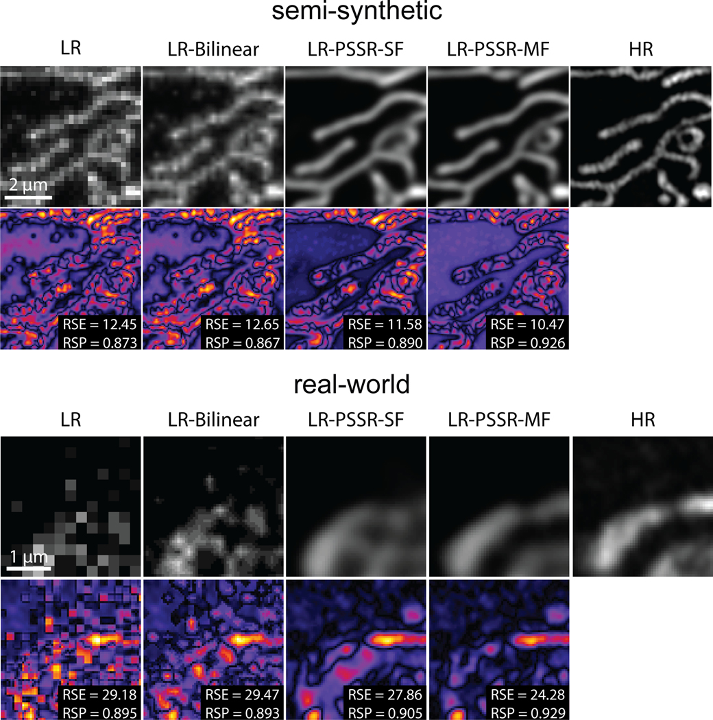
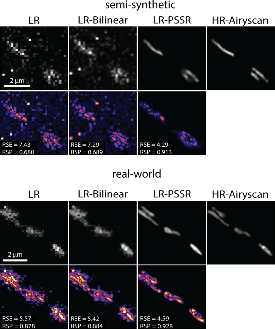
NanoJ-SQUIRREL²⁵ was used to calculate the RSE and RSP for both semi-synthetic and real-world acquired low (LR), bilinear interpolated (LR-Bilinear), and PSSR (LR-PSSR) images versus ground truth high-resolution (HR) images. Difference error maps were also calculated (Extended Data Fig. 2, 7 and 10).

EM Imaging and Analysis

tSEM high-resolution training data acquisition.

Tissue from a perfused 7-month old Long Evans male rat was cut from the left hemisphere, stratum radiatum of CA1 of the hippocampus. The tissue was stained, embedded, and sectioned at 45nm using previously described protocols⁵². Sections were imaged using a STEM detector on a ZEISS Supra 40 scanning electron microscope with a 28kV accelerating voltage and an extractor current of 102μA (gun aperture 30μm). Images were acquired with a 2nm pixel size and a field size of 24576 × 24576 pixels with Zeiss ATLAS. The working distance from the specimen to the final lens was 3.7mm, and the dwell time was 1.2μs.

EM testing sample preparation and image acquisition.

EM data sets were acquired from multiple systems at multiple institutions for this study.

For our testing ground truth data, paired LR and HR images of the adult mouse hippocampal dentate gyrus middle molecular layer neuropil were acquired from ultrathin sections (80nm) collected on silicon chips and imaged in a ZEISS Sigma VP FE-SEM²¹. All animal work was approved by the Institutional Animal Care and Use Committee (IACUC) of the Salk Institute for Biological Studies. Samples were prepared for EM according the NCMIR protocol⁵³. Pairs of 4 × 4μm images were collected from the same region at pixels sizes of both 8nm and 2nm using Fibics ATLAS software (InLens detector; 3kV; dwell time, 5.3μs; line averaging, 2; aperture, 30μm; working distance, 2mm).

Serial block face scanning electron microscope images were acquired with a Gatan 3View system installed on the ZEISS Sigma VP FE-SEM. Images were acquired using a pixel size of 8nm on a Gatan backscatter detector at 1kV and a current of 221pA. The pixel dwell time was 2μs with an aperture of 30μm and a working distance of 6.81mm. The section thickness was 100nm and the field of view was 24.5 × 24.5μm.

Mouse FIB-SEM data sample preparation and image acquisition settings were previously described in the original manuscript the datasets were published²². Briefly, the images were acquired with 4nm voxel resolution. We downsampled the lateral resolution to 8nm, then applied our PSSR model to the downsampled data to ensure the proper 8-to-2nm transformation for which the PSSR was trained.

Fly FIB-SEM data sample preparation and image acquisition settings were previously described in the original manuscript the datasets were published⁵⁴. Briefly, images were acquired with 10nm voxel resolution. We first upsampled the xy resolution to 8nm using bilinear interpolation, then applied our PSSR model to the upsampled data to ensure the proper 8-to-2nm transformation for which the PSSR model was originally trained.

The rat SEM data sample was acquired from an 8-week old male Wistar rat that was anesthetized with an overdose of pentobarbital (75 mg kg⁻¹) and perfused through the heart with 5 – 10ml of a solution of 250 mM sucrose 5mM MgCl₂ in 0.02 M phosphate buffer (pH 7.4) (PB) followed by 200 ml of 4% paraformaldehyde containing 0.2% picric acid and 1% glutaraldehyde in 0.1 M PB. Brains were then removed and oblique horizontal sections (50μm thick) of frontal cortex/striatum were cut on a vibrating microtome (Leica VT1200S, Nussloch, Germany) along the line of the rhinal fissure. The tissue was stained and cut to 50nm sections using ATUMtome (RMC Boeckeler, Tucson, USA) for SEM imaging using the protocol described in the original publication for which the data was acquired⁵⁵. The Hitachi Regulus rat SEM data was acquired using a Regulus 8240 FE-SEM with an acceleration voltage of 1.5kV, a dwell time of 3μs, using the backscatter detector with a pixel resolution of 10 × 10nm. We first upsampled the xy resolution to 8nm using bilinear interpolation, then applied our PSSR model to the upsampled data to ensure the proper 8-to-2nm transformation for which the PSSR model was originally trained.

EM segmentation and analysis.

Image sets generated from the same region of neuropil (LR-Bilinear; LR-PSSR; HR) were aligned rigidly using the ImageJ plugin Linear stack alignment with SIFT⁵⁶. Presynaptic axonal boutons (n = 10) were identified and cropped from the image set. The bouton image sets from the three conditions were then assigned randomly generated filenames and distributed to two blinded human experts for manual segmentation of presynaptic vesicles. Vesicles were identified by having a clear and complete membrane, being round in shape, and of approximately 35nm in diameter. For consistency between human experts, vesicles that were embedded in or attached to obliquely sectioned axonal membranes were excluded. Docked and non-docked synaptic vesicles were counted as separate pools. Vesicle counts were recorded and unblinded and grouped by condition and by expert counter. Linear regression analyses were conducted between the counts of the HR images and the corresponding images of the two different LR conditions (LR-Bilinear; LR-PSSR) to determine how closely the counts corresponded between the HR and LR conditions. Linear regression analysis was also used to determine the variability between counters.

Fluorescence Imaging and Analysis

U2OS cell culture.

U2OS cells were purchased from ATCC. Cells were grown in DMEM supplemented with 10% fetal bovine serum at 37 °C with 5% CO₂. Cells were plated onto either 8-well #1.5 imaging chambers or #1.5 35 mm dishes (Cellvis) coated with 10 μg/mL fibronectin in PBS at 37 °C for 30 minutes prior to plating. 50nm MitoTracker Deep Red or CMXRos Red (ThermoFisher) was added for 30 minutes then washed for at least 30 minutes to allow for recovery time before imaging in FluoroBrite (ThermoFisher) media.

Airyscan confocal imaging of U2OS cells.

To generate our ground truth training and testing dataset we used a ZEISS Airyscan LSM 880, an advanced confocal microscope that uses a 32-detector array and post-processing pixel reassignment to generate images ~1.7x higher in resolution (~120nm) and ~8x higher SNR than a standard confocal system. All HR ground truth training data were acquired with a 63x objective with at least 2x Nyquist sampling pixel sizes (~50±10nm pixels), then Airyscan processed (deconvolved) using ZEISS Zen software. For the real-world LR test data, we acquired images at 16x lower pixel resolution (~200nm pixel sizes) with a 2.5 AU pinhole on a PMT confocal detector, without any additional image processing. We maintained equal pixel dwell times for the HR versus LR testing acquisitions, resulting in overall 16x shorter exposure times for the LR images. To ensure minimal phototoxicity, we also decreased the laser power for our LR acquisitions by a factor of 4 or 5 (see Tables 1–2 for more details), resulting in a net laser dose decrease of ~64–80x (e.g., 5x lower laser power and 16x shorter exposure time yields a 80x lower laser dose). Furthermore, our LR testing data was not deconvolved and used a much larger effective pinhole size than the HR Airyscan ground truth data, resulting in a blurrier image with lower optical resolution. Cells were imaged with a 63× 1.4 NA oil objective on a ZEISS 880 LSM Airyscan confocal system with an inverted stage and heated incubation system with 5% CO₂ control. For both HR and LR images, equal or lower (when indicated) laser power and equal pixel dwell time of ~1 μs/pixel was used. For testing PSSR-MF, at least 10 sequential frames of fixed samples were acquired with high- and low-resolution settings in order to facilitate PSSR-MF processing.

Neuron preparation.

Primary hippocampal neurons were prepared from E18 rat (Envigo) embryos as previously described. Briefly, hippocampal tissue was dissected from embryonic brain and further dissociated to single hippocampal neuron by trypsinization with Papain (Roche). The prepared neurons were plated on coverslips (Bellco Glass) coated with 3.33μg/mL laminin (Life Technologies) and 20μg/mL poly-L-Lysine (Sigma) at the density of 7.5 × 10⁴ cells/cm². The cells were maintained in Neurobasal medium supplemented with B27 (Life Technologies), penicillin/streptomycin and L-glutamine for 7 – 21 days in vitro. Two days before imaging, the hippocampal neurons were transfected with Lipofectamine 2000 (Life Technologies).

Temporal consistency analysis.

Given a preprocessed time-lapse movie with $N$ total number of frames, the cross-correlation coefficient ($\varnothing \left(X_i, X_{i+1}\right), iϵ[1, N)$) was calculated for two neighboring frames ($X_i$ and $X_{i+1}$) repeatedly across each movie with a step size of $i=1$ (Fig. 4b). To ensure comparisons between PSSR output and ground truth data were not biased by high frequency artifacts and noise, each time-lapse was first preprocessed with a Gaussian blur filter ($\sigma =5).$

Fission event detection and analysis.

Given fission events cannot be precisely defined across different evaluators, a HR timelapse of mitotracker stained cells was first given to two human experts as a pilot experiment to examine and correct the inspection performance of all experts. Three conditions (LR-Bilinear; LR-PSSR; HR) of the same Airyscan timelapses (n = 6) were then sequentially assigned to two blinded human experts for mitochondria fission event detection. Fission event counts were recorded and unblinded and grouped by condition and by expert counter. Linear regression analyses were conducted between the counts of the HR images and the corresponding images of the two different LR conditions (LR-Bilinear; LR-PSSR) to determine how closely the counts corresponded between the HR and LR conditions. Linear regression analysis was used to determine the variability between counters.

Neuronal mitochondria imaging and kymograph analysis.

Live-cell imaging of primary neurons was performed using a Zeiss LSM 880 confocal microscope, enclosed in a temperature control chamber at 37 °C and 5% CO₂, using a 63x (NA 1.4) oil objective in SR-Airyscan mode (i.e. 0.2 AU virtual pinhole). For low-resolution conditions, images were acquired with a confocal PMT detector with a pinhole size of 2.5 AU at 440 × 440 pixels at 0.5x Nyquist (170nm/pixel) every 270.49ms using a pixel dwell time of 1.2μs and a laser power ranging between 1 – 20 μW. For high-resolution conditions, images were acquired at 1764 × 1764 pixels at 2x Nyquist (~42nm/pixel) every 4.33s using a pixel dwell time of 1.2μs and a laser power of 20μW. Imaging data were collected using Zen Black software. High-resolution images were further processed using Zen Blue’s 2D-SR Airyscan processing. Kymograph analysis of the time-lapse movies were conducted using ImageJ plugin Kymolyzer as described previously⁵⁷.

Fluorescence photobleaching quantification.

Normalized mean intensity over time was measured using Fiji software. Given a time-lapse movie with $N$ frames, a background region was randomly selected and remained unchanged across frames. The normalized mean intensity (${\stackrel{-}{I}}_{norm}^{\left(i\right)}$) can be expressed as:

$${\stackrel{-}{I}}_{norm}^{\left(i\right)}=\frac{{\stackrel{-}{I}}_{img}^{\left(i\right)}-{\stackrel{-}{I}}_{bg}^{\left(i\right)}}{MAX({\stackrel{-}{I}}_{img}^{\left(i\right)}-{\stackrel{-}{I}}_{bg}^{\left(i\right)})},\mathrm{ }i\in \left[1,N\right]$$

where $i$ represents the frame index, ${\stackrel{-}{I}}_{bg}^{\left(i\right)}$ represents the mean intensity of the selected background region at frame $i$ and ${\stackrel{-}{I}}_{img}^{\left(i\right)}$ represents the intensity mean of the entire frame $i$.

Comparing PSSR with other methods

Block-matching and 3D filtering (BM3D) denoising algorithm.

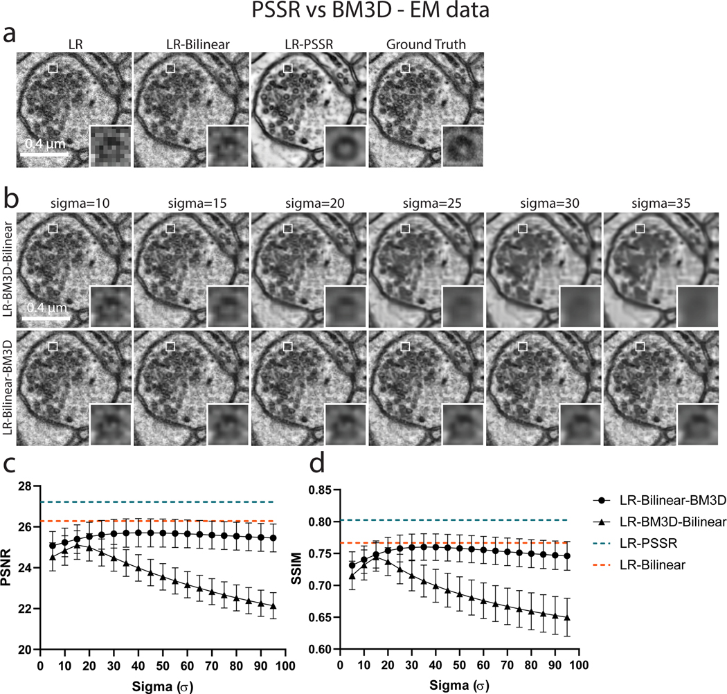
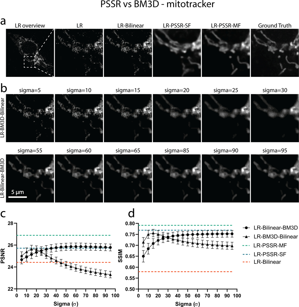
We compared PSSR with BM3D, on both EM and fluorescence MitoTracker data. Application of BM3D before (LR-BM3D-Bilinear) and after (LR-Bilinear-BM3D) bilinear upsampling of pixel sizes were both tested. A wide range of Sigma ($\sigma \in \left(0,\mathrm{ }95\right]$), the key parameter that defines the assumed zero-mean white Gaussian noise in the images, was thoroughly explored. The exact same test set was used for quantification of PSSR vs. BM3D results.

Content-aware Image Restoration (CARE) and Rolling Average (RA) methods.

A semi-synthetically crappified dataset of MitoTracker data was used to train both CARE and PSSR networks (PSSR-SF and PSSR-MF) in a consistent manner. We applied the trained models to semi-synthetically generated low-resolution testing time-lapses. Testing data were similarly crappified as training data. Five-frame rolling average processing was further applied to CARE and single-frame testing output.

Data Availability

Example training data and pretrained models are included in the GitHub release (https://github.com/BPHO-Salk/PSSR). The entirety of our training and testing data sets and data sources are available at Texas Data Repository (https://doi.org/10.18738/T8/YLCK5A).

Code Availability

PSSR source code and documentation are available for download on GitHub (https://github.com/BPHO-Salk/PSSR) and are free for use under the BSD 3-Clause License.

Reporting summary

Further information on research design is available in the Life Sciences Reporting Summary linked to this article.

Extended Data

Extended Data Fig. 1. PSSR Neural Network architecture.

Shown is the ResNet-34 based U-Net architecture. Single-frame PSSR (PSSR-SF) and multi-frame PSSR (PSSR-MF) have 1 or 5 input channels, separately.

Extended Data Fig. 2. NanoJ-SQUIRREL error-maps of EM data.

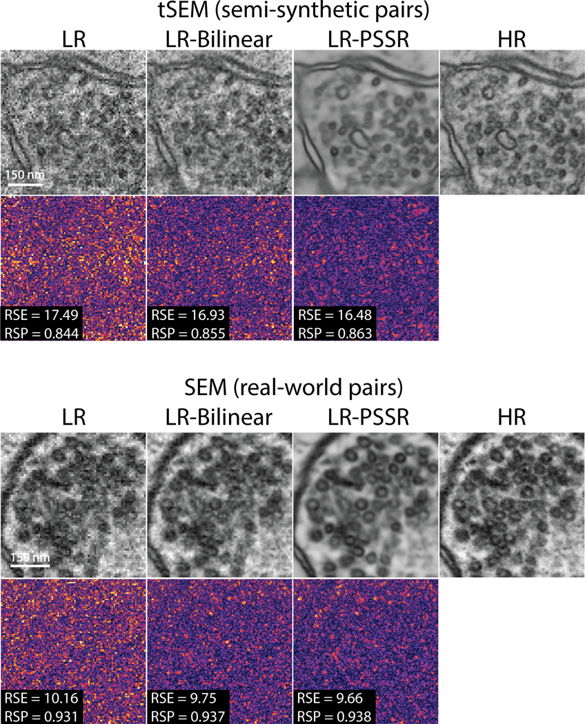
NanoJ-SQUIRREL was used to calculate the resolution scaled error (RSE) and resolution scaled Pearson’s coefficient (RSP) for both semi-synthetic and real-world acquired low (LR), bilinear interpolated (LR-Bilinear), and PSSR (LR-PSSR) images versus ground truth high-resolution (HR) images. For these representative images from Fig. 2, the RSE and RSP images are shown along with the difference images for each output.

Extended Data Fig. 3. Comparison of PSSR vs. BM3D on EM data.

PSSR restoration was compared to the Block-matching and 3D filtering (BM3D) denoising algorithm. BM3D was applied to low-resolution real-world SEM images before (LR-BM3D-Bilinear) and after (LR-Bilinear-BM3D) bilinear upsampling. A wide range of Sigma ($\sigma \in \left(0,\mathrm{ }95\right]$, with step size of 5), the key parameter that defines the assumed zero-mean white Gaussian noise in BM3D method, was thoroughly explored. Images of the same region from the LR input, bilinear upsampled, PSSR restored, and Ground truth is displayed in (a). Results of LR-BM3D-Bilinear (b, top row) and LR-Bilinear-BM3D (b, bottom row) with sigma ranging from [10, 15, … , 35] are shown. PSNR and SSIM results of LR-BM3D-Bilinear and LR-Bilinear-BM3D across the explored range of sigma are plotted in (c) and (d). Metrics for bilinear-upsampled and PSSR-restored images of the same testing set are shown as dashed lines in orange (LR-Bilinear: PSNR=26.28±0.085; SSIM=0.767±0.0031) and blue (LR-PSSR: PSNR=27.21±0.084; SSIM=0.802 ±0.0026). n=12 independent images for all conditions. Values are shown as mean ± SEM.

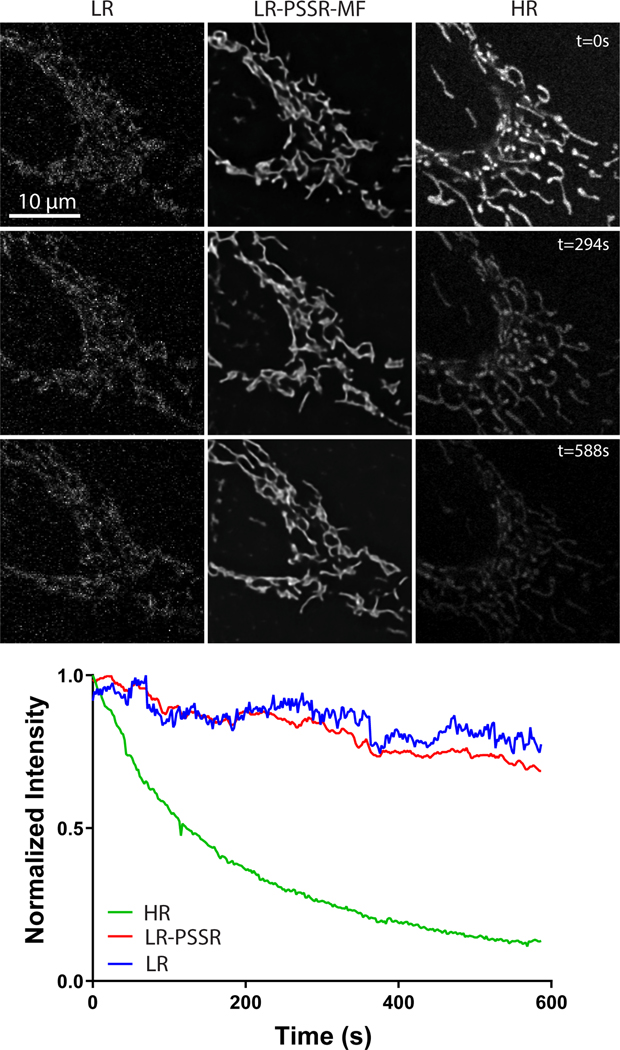
Extended Data Fig. 4. Undersampling significantly reduces photobleaching.

U2OS cells stained with mitotracker were imaged every 2 seconds with the same laser power (2.5μW) and pixel dwell time (~1μs), but with 16x lower resolution (196 × 196nm xy pixel size) than full resolution Airyscan acquisitions (~49 × 49nm xy pixel size). Mean intensity plots show the relative rates of fluorescence intensity loss over time (i.e. photobleaching) for LR, LR-PSSR, and HR images.

Extended Data Fig. 5. Evaluation of crappifiers with different noise injection on mitotracker data.

Examples of crappified training images, visualized results and metrics (PSNR, SSIM and FRC resolution) of PSSR-SF models that were trained on high- and low-resolution pairs semi-synthetically generated by crappifiers with different noise injection were presented. a, Shown is an example of crappified training images generated by different crappifiers, including “No noise” (no added noise, downsampled pixel size only), Salt & Pepper, Gaussian, Additive Gaussian, and a mixture of Salt & Pepper plus Additive Gaussian noise. High-resolution version of the same region is also included. b, Visualized restoration performance of PSSR models that used different crappifiers (No noise, Salt & Pepper, Gaussian, Additive Gaussian, and a mixture of Salt & Pepper plus Additive Gaussian noise). LR input and Ground Truth of the example testing ROI are also shown. PSNR (c), SSIM (d) and FRC (e) quantification show the PSSR model that used “Salt & Pepper + Additive Gaussian” crappifier yielded the best overall performance (n=10 independent timelapses of fixed samples with n=10 timepoints for all conditions). All values are shown as mean ± SEM. P values are specified in the figure for 0.0001<p<0.05. *p<0.05, **p<0.01, ***p<0.001, ****p<0.0001, ns = not significant; Two-sided paired t-test.

Extended Data Fig. 6. Quantitative comparison of CARE and PSSR-SF with PSSR-MF and Rolling Average (RA) methods for timelapse data.

PSNR (a) and SSIM (b) quantification show a decrease in accuracy when applying RA to LR-CARE and LR-PSSR-SF, while multi-frame PSSR provides superior performance compared to LR-PSSR-SF and CARE before and after RA processing. Data points were color-coded based on different cells. See Fig. 4c for visualized comparisons, and Supplementary Movie 6 for a video comparison of the entire timelapse for CARE, LR-PSSR-SF, LR-PSSR-SF-RA, and LR-PSSR-MF. N=5 independent timelapses with n=30 timepoints each, achieving similar results. All values are shown as mean ± SEM. ****p<0.0001; Two-sided paired t-test.

Extended Data Fig. 7. NanoJ-SQUIRREL error-maps of MitoTracker data.

NanoJ-SQUIRREL was used to calculate the resolution scaled error (RSE) and resolution scaled Pearson’s coefficient (RSP) for both semi-synthetic and real-world acquired low (LR), bilinear interpolated (LR-Bilinear), and PSSR (LR-PSSR) images versus ground truth high-resolution (HR) images. For these representative images from Fig. 4, the RSE and RSP images are shown along with the difference images for each output.

Extended Data Fig. 8. Compare PSSR with BM3D denoising method on mitotracker data.

PSSR restored images was compared to results of applying BM3D denoising algorithm to low-resolution real-world mitotracker images before (LR-BM3D-Bilinear) and after (LR-Bilinear-BM3D) bilinear upsampling. A wide range of Sigma ($\sigma \in \left(0,\mathrm{ }95\right]$, with step size of 5) was thoroughly explored. Examples of the same region from the LR input, bilinear upsampled, PSSR-SF restored, PSSR-MF restored, and Ground truth are displayed (a, top row). Images from the top 6 results (evaluated by both PSNR and SSIM values) of LR-BM3D-Bilinear (a, middle row) and LR-Bilinear-BM3D (a, bottom row) are shown. PSNR and SSIM results of LR-BM3D-Bilinear and LR-Bilinear-BM3D across the explored range of sigma are plotted in (b) and (c). Metrics resulted from bilinearly upsampled, PSSR-SF restored and PSSR-MF restored images of the same testing set are shown as dash lines in orange (LR-Bilinear: PSNR=24.42±0.367; SSIM=0.579 ±0. 0287), blue (LR-PSSR-SF: PSNR=25.72±0.323; SSIM=0.769 ±0.0139) and green (LR-PSSR-MF: PSNR=26.89 ±0.322; SSIM=0.791±0.0133). As it shows, in this fluorescence mitotracker example, BM3D performs better than bilinear upsampling with carefully defined noise distribution, whereas its general performance given both PSNR and SSIM is overall worse than single-frame PSSR (LR-PSSR-SF). Excitably, our multi-frame PSSR (LR-PSSR-MF) yields the best performance. n=10 independent timelapses of fixed samples with n=6–10 timepoints each for all conditions. Values are shown as mean ± SEM.

Extended Data Fig. 9. NanoJ-SQUIRREL error-maps of neuronal mitochondria data.

NanoJ-SQUIRREL was used to calculate the resolution scaled error (RSE) and resolution scaled Pearson’s coefficient (RSP) for both semi-synthetic and real-world acquired low (LR), bilinear interpolated (LR-Bilinear), and PSSR (LR-PSSR) images versus ground truth high-resolution (HR) images. For these representative images from Fig. 5, the RSE and RSP images are shown along with the difference images for each output.

Extended Data Fig. 10. PSSR facilitates detection of mitochondrial motility and dynamics.

Rat hippocampal neurons expressing mito-dsRed were undersampled with a confocal detector using 170nm pixel resolution (LR) to facilitate faster frame rates, then restored with PSSR (LR-PSSR). a, before and after time points of the event shown in Fig. 5 wherein two adjacent mitochondria pass one another but cannot be resolved in the original low-resolution (LR) or bilinear interpolated (LR-Bilinear) image but are clearly resolved in the LR-PSSR image. b, kymographs of a LR vs LR-PSSR timelapse that facilitates the detection of a mitochondrial fission event (yellow arrow).

Supplementary Material

1668081_SourceDataFig5

Statistical source data for PSNR, SSIM and FRC resolution plots of both semi-synthetic and real-world testing data (panel b) and mitochondrion mobility analysis plots (panel f-i)

1668081_SourceExtDataFig5

Statistical source data for PSNR, SSIM and FRC resolution plots (panel c-e)

1668081_SourceExtDataFig4

Source data for photobleaching intensity plots.

1668081_SourceDataFig4

Statistical source data for flickering quantification plots (panel b), PSNR, SSIM and FRC resolution plots (panel f) and fission event counting plots (panel h-k)

1668081_SourceExtDataFig6

Statistical source data for PSNR and SSIM plots (panel a-b)

1668081_SourceExtDataFig8

Statistical source data for PSNR and SSIM plots (panel c-d)

1668081_SourceExtDataFig3

Statistical source data for PSNR and SSIM plots (panel c-d)

References

- 1.Wang Z, Chen J & Hoi SCH Deep Learning for Image Super-resolution: A Survey. eprint arXiv:1902.06068, arXiv:1902.06068 (2019). [DOI] [PubMed] [Google Scholar]
- 2.Jain V et al. Supervised Learning of Image Restoration with Convolutional Networks. (2007). [Google Scholar]
- 3.Romano Y, Isidoro J & Milanfar P. RAISR: rapid and accurate image super resolution. IEEE Transactions on Computational Imaging 3, 110–125 (2016). [Google Scholar]
- 4.Shrivastava A et al. in Proceedings of the IEEE conference on computer vision and pattern recognition. 2107–2116. [Google Scholar]
- 5.Moen E et al. Deep learning for cellular image analysis. Nat Methods, doi: 10.1038/s41592-019-0403-1 (2019). [DOI] [PMC free article] [PubMed] [Google Scholar]
- 6.Buchholz T-O, Jordan M, Pigino G & Jug F in 2019 IEEE 16th International Symposium on Biomedical Imaging (ISBI 2019). 502–506 (IEEE; ). [Google Scholar]
- 7.Krull A, Buchholz T-O & Jug F in Proceedings of the IEEE Conference on Computer Vision and Pattern Recognition. 2129–2137. [Google Scholar]
- 8.Buchholz TO et al. Content-aware image restoration for electron microscopy. Methods Cell Biol 152, 277–289, doi: 10.1016/bs.mcb.2019.05.001 (2019). [DOI] [PubMed] [Google Scholar]
- 9.Weigert M et al. Content-aware image restoration: pushing the limits of fluorescence microscopy. Nat Methods 15, 1090–1097, doi: 10.1038/s41592-018-0216-7 (2018). [DOI] [PubMed] [Google Scholar]
- 10.Batson J & Royer L. Noise2self: Blind denoising by self-supervision. arXiv preprint arXiv:1901.11365 (2019). [Google Scholar]
- 11.Li Y et al. DLBI: deep learning guided Bayesian inference for structure reconstruction of super-resolution fluorescence microscopy. Bioinformatics 34, i284-i294, doi: 10.1093/bioinformatics/bty241 (2018). [DOI] [PMC free article] [PubMed] [Google Scholar]
- 12.Ouyang W, Aristov A, Lelek M, Hao X & Zimmer C. Deep learning massively accelerates super-resolution localization microscopy. Nat Biotechnol 36, 460–468, doi: 10.1038/nbt.4106 (2018). [DOI] [PubMed] [Google Scholar]
- 13.Nelson AJ & Hess ST Molecular imaging with neural training of identification algorithm (neural network localization identification). Microsc Res Tech 81, 966–972, doi: 10.1002/jemt.23059 (2018). [DOI] [PMC free article] [PubMed] [Google Scholar]
- 14.Heinrich L, Bogovic JA & Saalfeld S in Medical Image Computing and Computer-Assisted Intervention − MICCAI 2017. (eds Maxime Descoteauxet al.) 135–143 (Springer International Publishing; ). [Google Scholar]
- 15.de Haan K, Ballard ZS, Rivenson Y, Wu Y & Ozcan A. Resolution enhancement in scanning electron microscopy using deep learning. Scientific Reports 9, 1–7 (2019). [DOI] [PMC free article] [PubMed] [Google Scholar]
- 16.Sreehari S et al. in Proceedings of the IEEE Conference on Computer Vision and Pattern Recognition Workshops. 88–96. [Google Scholar]
- 17.Wang H et al. Deep learning enables cross-modality super-resolution in fluorescence microscopy. Nat Methods 16, 103–110, doi: 10.1038/s41592-018-0239-0 (2019). [DOI] [PMC free article] [PubMed] [Google Scholar]
- 18.Chen J et al. Three-dimensional residual channel attention networks denoise and sharpen fluorescence microscopy image volumes. bioRxiv, 2020.2008.2027.270439, doi: 10.1101/2020.08.27.270439 (2020). [DOI] [PubMed] [Google Scholar]
- 19.Guo M et al. Rapid image deconvolution and multiview fusion for optical microscopy. Nat Biotechnol, doi: 10.1038/s41587-020-0560-x (2020). [DOI] [PMC free article] [PubMed] [Google Scholar]
- 20.Kobayashi H, Solak AC, Batson J & Royer LA Image Deconvolution via Noise-Tolerant Self-Supervised Inversion. arXiv preprint arXiv:2006.06156 (2020). [Google Scholar]
- 21.Horstmann H, Korber C, Satzler K, Aydin D & Kuner T. Serial section scanning electron microscopy (S3EM) on silicon wafers for ultra-structural volume imaging of cells and tissues. PLoS One 7, e35172, doi: 10.1371/journal.pone.0035172 (2012). [DOI] [PMC free article] [PubMed] [Google Scholar]
- 22.Xu CS et al. Enhanced FIB-SEM systems for large-volume 3D imaging. Elife 6, doi: 10.7554/eLife.25916 (2017). [DOI] [PMC free article] [PubMed] [Google Scholar]
- 23.Denk W & Horstmann H. Serial block-face scanning electron microscopy to reconstruct three-dimensional tissue nanostructure. PLoS Biol 2, e329, doi: 10.1371/journal.pbio.0020329 (2004). [DOI] [PMC free article] [PubMed] [Google Scholar]
- 24.Kuwajima M, Mendenhall JM, Lindsey LF & Harris KM Automated transmission-mode scanning electron microscopy (tSEM) for large volume analysis at nanoscale resolution. PLoS One 8, e59573, doi: 10.1371/journal.pone.0059573 (2013). [DOI] [PMC free article] [PubMed] [Google Scholar]
- 25.Culley S et al. Quantitative mapping and minimization of super-resolution optical imaging artifacts. Nat Methods 15, 263–266, doi: 10.1038/nmeth.4605 (2018). [DOI] [PMC free article] [PubMed] [Google Scholar]
- 26.Dabov K, Foi A, Katkovnik V & Egiazarian K in Image Processing: Algorithms and Systems, Neural Networks, and Machine Learning. 606414 (International Society for Optics and Photonics; ). [Google Scholar]
- 27.von Chamier L, Laine RF & Henriques R. Artificial intelligence for microscopy: what you should know. Biochem Soc Trans, doi: 10.1042/BST20180391 (2019). [DOI] [PubMed] [Google Scholar]
- 28.Belthangady C & Royer LA Applications, promises, and pitfalls of deep learning for fluorescence image reconstruction. Nat Methods, doi: 10.1038/s41592-019-0458-z (2019). [DOI] [PubMed] [Google Scholar]
- 29.Phototoxicity revisited. Nat Methods 15, 751, doi: 10.1038/s41592-018-0170-4 (2018). [DOI] [PubMed] [Google Scholar]
- 30.Jonkman J & Brown CM Any Way You Slice It-A Comparison of Confocal Microscopy Techniques. J Biomol Tech 26, 54–65, doi: 10.7171/jbt.15-2602-003 (2015). [DOI] [PMC free article] [PubMed] [Google Scholar]
- 31.Kner P, Chhun BB, Griffis ER, Winoto L & Gustafsson MG Super-resolution video microscopy of live cells by structured illumination. Nat Methods 6, 339–342, doi: 10.1038/nmeth.1324 (2009). [DOI] [PMC free article] [PubMed] [Google Scholar]
- 32.Wronski B et al. Handheld Multi-Frame Super-Resolution. arXiv preprint arXiv:1905.03277 (2019). [Google Scholar]
- 33.Huang X et al. Fast, long-term, super-resolution imaging with Hessian structured illumination microscopy. Nat Biotechnol 36, 451–459, doi: 10.1038/nbt.4115 (2018). [DOI] [PubMed] [Google Scholar]
- 34.Carlton PM et al. Fast live simultaneous multiwavelength four-dimensional optical microscopy. Proc Natl Acad Sci U S A 107, 16016–16022, doi: 10.1073/pnas.1004037107 (2010). [DOI] [PMC free article] [PubMed] [Google Scholar]
- 35.Arigovindan M et al. High-resolution restoration of 3D structures from widefield images with extreme low signal-to-noise-ratio. Proc Natl Acad Sci U S A 110, 17344–17349, doi: 10.1073/pnas.1315675110 (2013). [DOI] [PMC free article] [PubMed] [Google Scholar]
- 36.Barbastathis G, Ozcan A & Situ G. On the use of deep learning for computational imaging. Optica 6, 921–943, doi: 10.1364/OPTICA.6.000921 (2019). [DOI] [Google Scholar]
- 37.Keren L et al. MIBI-TOF: A multiplexed imaging platform relates cellular phenotypes and tissue structure. Sci Adv 5, eaax5851, doi: 10.1126/sciadv.aax5851 (2019). [DOI] [PMC free article] [PubMed] [Google Scholar]
- 38.Arrojo EDR et al. Age Mosaicism across Multiple Scales in Adult Tissues. Cell Metab 30, 343–351 e343, doi: 10.1016/j.cmet.2019.05.010 (2019). [DOI] [PMC free article] [PubMed] [Google Scholar]
- 39.Wolf SG & Elbaum M. CryoSTEM tomography in biology. Methods Cell Biol 152, 197–215, doi: 10.1016/bs.mcb.2019.04.001 (2019). [DOI] [PubMed] [Google Scholar]
Methods-only References
- 40.Perez L & Wang J. The effectiveness of data augmentation in image classification using deep learning. arXiv preprint arXiv:1712.04621 (2017). [Google Scholar]
- 41.Ronneberger O, Fischer P & Brox T in International Conference on Medical image computing and computer-assisted intervention. 234–241 (Springer; ). [Google Scholar]
- 42.Shi W et al. in Proceedings of the IEEE conference on computer vision and pattern recognition. 1874–1883. [Google Scholar]
- 43.Harada Y, Muramatsu S & Kiya H in 9th European Signal Processing Conference (EUSIPCO 1998). 1–4 (IEEE; ). [Google Scholar]
- 44.Sugawara Y, Shiota S & Kiya H in 2018 25th IEEE International Conference on Image Processing (ICIP). 66–70 (IEEE; ). [Google Scholar]
- 45.Aitken A et al. Checkerboard artifact free sub-pixel convolution: A note on sub-pixel convolution, resize convolution and convolution resize. arXiv preprint arXiv:1707.02937 (2017). [Google Scholar]
- 46.Zhang H, Goodfellow I, Metaxas D & Odena A. Self-attention generative adversarial networks. arXiv preprint arXiv:1805.08318 (2018). [Google Scholar]
- 47.Loshchilov I & Hutter F. Sgdr: Stochastic gradient descent with warm restarts. arXiv preprint arXiv:1608.03983 (2016). [Google Scholar]
- 48.Smith LN in 2017 IEEE Winter Conference on Applications of Computer Vision (WACV). 464–472 (IEEE; ). [Google Scholar]
- 49.Smith LN A disciplined approach to neural network hyper-parameters: Part 1--learning rate, batch size, momentum, and weight decay. arXiv preprint arXiv:1803.09820 (2018). [Google Scholar]
- 50.Smith LN & Topin N Super-convergence: Very fast training of residual networks using large learning rates. (2018). [Google Scholar]
- 51.Hore A & Ziou D in 2010 20th International Conference on Pattern Recognition. 2366–2369 (IEEE; ). [Google Scholar]
- 52.Kuwajima M, Mendenhall JM & Harris KM Large-volume reconstruction of brain tissue from high-resolution serial section images acquired by SEM-based scanning transmission electron microscopy. Methods Mol Biol 950, 253–273, doi: 10.1007/978-1-62703-137-0_15 (2013). [DOI] [PMC free article] [PubMed] [Google Scholar]
- 53.Deerinck TJ, Bushong EA, Thor A & Ellisman MH NCMIR methods for 3D EM: a new protocol for preparation of biological specimens for serial block face scanning electron microscopy. Microscopy, 6–8 (2010). [Google Scholar]
- 54.Takemura SY et al. Synaptic circuits and their variations within different columns in the visual system of Drosophila. Proc Natl Acad Sci U S A 112, 13711–13716, doi: 10.1073/pnas.1509820112 (2015). [DOI] [PMC free article] [PubMed] [Google Scholar]
- 55.Kubota Y et al. A carbon nanotube tape for serial-section electron microscopy of brain ultrastructure. Nat Commun 9, 437, doi: 10.1038/s41467-017-02768-7 (2018). [DOI] [PMC free article] [PubMed] [Google Scholar]
- 56.Lowe DG Distinctive Image Features from Scale-Invariant Keypoints. International Journal of Computer Vision 60, 91–110, doi: 10.1023/b:Visi.0000029664.99615.94 (2004). [DOI] [Google Scholar]
- 57.Pekkurnaz G, Trinidad JC, Wang X, Kong D & Schwarz TL Glucose regulates mitochondrial motility via Milton modification by O-GlcNAc transferase. Cell 158, 54–68, doi: 10.1016/j.cell.2014.06.007 (2014). [DOI] [PMC free article] [PubMed] [Google Scholar]
Associated Data
This section collects any data citations, data availability statements, or supplementary materials included in this article.
Supplementary Materials