Spatial analysis of COVID-19 incidence and its determinants using spatial modeling: A study on India

Abstract

The first incident of COVID-19 case in India was recorded on 30th January, 2020 which turns to 100,000 marks on May 19th and by June 3rd it was over 200,000 active cases and 5,800 deaths. Geographic Information System (GIS) based spatial models can be helpful for better understanding of different factors that have triggered COVID-19 spread at district level in India. In the present study, 19 variables were considered that can explain the variability of the disease. Different spatial statistical techniques were used to describe the spatial distribution of COVID-19 and identify significant clusters. Spatial lag and error models (SLM and SEM) were employed to examine spatial dependency, geographical weighted regression (GWR) and multi-scale GWR (MGWR) were employed to examine at local level. The results show that the global models perform poorly in explaining the factors for COVID-19 incidences. MGWR shows the best-fit-model to explain the variables affecting COVID-19 (R2= 0.75) with lowest AICc value. Population density, urbanization and bank facility were found to be most susceptible for COVID-19 cases. These indicate the necessity of effective policies related to social distancing, low mobility. Mapping of different significant variables using MGWR can provide significant insights for policy makers for taking necessary actions.

1. Introduction

The pandemic of this century which is created by the COVID-19, has become a major challenge to the nations. As of June 5th 2020, more than 6,704,010 peoples are reported positive worldwide and more than 393,233 peoples lost their life due to COVID-19. Following the devastating impact of this infectious virus, the United Nations has declared the situation as human, economic, and social crisis (United Nations. Department of Economic and Social Affairs Social Inclusion. 2020). As per record of the World Health Organization, this virus was first observed in the Wuhan city of China. Later on, the virus has moved in different countries through human body transmission and the international passengers have worked as the carrier unknowingly and unintentionally (Lau et al., 2020). India, a south Asian country, has also affected critically by this. Initially, the number of corona virus positive case was very low in India and the Government of India has undertaken several crucial steps immediately to stop the spread of this virus in the country (Tata Capital blog, 2020). However, despite of several actions like suspension of visas, shut down of all educational institutions, compulsory 14 days of isolation of people who had travelled abroad, taking samples for COVID test etc., the number of positive cases in India is increasing gradually. Currently, each day India registers record number of positive cases and, most importantly, the report of positive cases are coming out almost from every state. As of June 5^th, 2020, more than 0.22 million confirmed cases have been reported in India. Though the number of cases is not very high in respect to the entire country's population size at present, it becomes crucial in terms of its intensity and increasing rate. Therefore, the number of positive cases will likely to increase in the upcoming days. Besides, due to the high negative impact of lockdown on the country's economy, the Government of India has decided to end the lockdown in the country phase wise on and from June 1st, 2020. It will also lead to the increase in the number of positive cases at a rapid speed.

Recent researches regarding COVID-19 had identified multiple factors associated with this incident, such as, temperature (Liu et al., 2020; Wang et al., 2020; Yongjiana et al., 2020; Zhu and Xie, 2020), air pollution (Wu et al., 2020), humidity (Auler et al., 2020; Gupta et al., 2020; Ma et al., 2020), smoking (Taghizadeh-Hesary and Akbari, 2020) and WaSH effects (Das et al., 2020), social vulnerability (Kang et al., 2020) which may regulate the severity and rate of COVID-19 spread. Identification of risk factors related to demographic, socio-economic, building environment is essential at every phase of this pandemic for all practical purpose of preventing the spread of COVID-19 virus. It is already observed that poor demographic, socio-economic, building environment, poor health structure are considered possible factors for spreading infectious diseades like HIV, Influenza, Tuberculosis, Pneumonia etc. (Khalatbari-Soltani et al., 2020; Bluhm and Pinkovskiy, 2020; Bärnighausen et al., 2020; Huang et al., 2017; Farr et al., 2000). These studies may suggest that similar pattern might be visible for this newly emerged virus. However, more studies are needed in context of developing countries in different contexts that considers large variety of determinants for getting a complete scenario. Developing country like India with huge population of 1.38 billion faces major problems in different issues like lack of proper infrastructure, unemployment, social inequality, poor health structures etc, could be a perfect unit of study for understanding different contributing factors of COVID-19. Moreover, most of the studies do not emphasize these important factors which need to be explored to gain more awareness about this pandemic. Therefore the main question arise here is that what is the potential impact of demographic, socio-economic, building environment or health structure on COVID-19 incidence.

GIS is an excellent platform to examine the spatial epidemiology and mapping of infectious diseases. Spatial statistics and mapping can aid the process of providing insights to fight against a pandemic and improving public health (Mollalo et al., 2020; Ramírez-Aldana et al., 2020). Very few researches had been made using GIS technique regarding the vectors of COVID-19 pandemic (Das et al., 2020; Das et al., 2020b; Gibson and Rush, 2020; Lakhani, 2020).

Spatial statistics tools are excellent way to investigate the relationship between different independent variables and COVID-19 disease outbreak (Ramírez-Aldana et al., 2020). In this study, different spatial analysis and regression models were performed to examine the COVID-19 situation in India and how well the models can explain the vectors of COVID-19 outbreak in India considering different explanatory variables. This study in India with respect to COVID-19 will be helpful in (i) accessing the role of different influencing factors to the practitioners and administrators; (ii) addressing the spatial vulnerability of the community to the COVID-19 district-wise; (iii) development of effective mitigation strategies.

2. Data and methodology

2.1. Study area

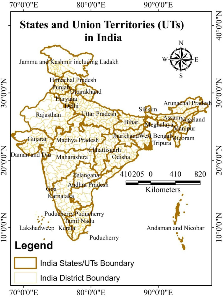
India, a country of South Asia with 1.38 billion people (https://www.worldometers.info), is the second largest populous country in the world. As per the Census of India 2011, the population density in India is 382 persons/sq. km, which is comparatively very high concerning the western world. This country is very vulnerable to the spread of corona virus due to very dense population. Therefore, it becomes essential to find out the role of different factors that are associated with high possibility of the spreading of the virus. India is composed of 640 districts (Census of India 2011). This study is conducted in case of the whole India (Fig. 1).

Fig. 1.

Location of India with all states and Union territories (UTs).

2.2. Data collection

For this study, relevance data were collected from different official websites. District level COVID-19 cases across the country were retrieved from https://www.covid19india.org on June 3rd, 2020. COVID-19 data was used as the dependent variable.

A list of 19 variables (Table 1 ) categorized into three broad dimensions namely adaptive, sensitivity and exposure were considered. These variables are related to the demographic, economic, health facilities, community facilities, building environment etc. As discussed earlier these variables may be considered as the explanatory factors for COVID-19 cases.

Table 1.

List of variables taken as explanatory variables in the study.

Dimension	Indicator	Source	Description
Adaptive	Availability of health facility per lakh	District wise RHS data, 2019
	Availability of banking facility	Census of India, 2011
	Literacy rate	Census of India, 2011
	Asset index	Census of India, 2011	Average of HHs have Radio/Transistor, Television, computer/laptop, telephone/mobile, bicycle, Scooter/ Motorcycle/Moped, Car/ Jeep/Van
	Housing index (good condition, permanent hh, own)	Census of India, 2011	Average of HHs have good condition of house, permanent house and own house
	% of population have very high blood sugar	NFHS 4	Includes both male and female
	% of population have very high hypertension	NFHS 4	Includes both male and female
Sensitivity	Percentage of population of age 60 and more	NFHS 4
	Percentage of population of age 6 and less	Census of India, 2011
	% of HH having water inside premises	Census of India, 2011
	% of HH having sanitation inside premises	Census of India, 2011
	% of Households use clean source of fuel	Census of India, 2011	Fuel sources that do not cause much pollution to the environment
	% of Households having electricity	Census of India, 2011
Exposure	Max temperature	World climate
	Min temperature	World climate
	Precipitation	World climate
	Urbanization rate	Census of India, 2011	Percentage of urban population to total population
	Household density	Census of India, 2011
	Population density	Census of India, 2011

2.3. Spatial autocorrelation

Moran's I statistics was used to estimate the global autocorrelation and spatial distribution of COVID-19 cases and different variables. Moran's I helps to understand the distribution pattern. The outcome of the analysis is produced in two types of map, LISA cluster map and LISA significant map. LISA cluster map were generated to understand the contribution of each district in the analysis. LISA cluster types are: high-high (HH), low-low (LL), low-high (LH) and high-low (HL). HH and LL clusters indicate significant clusters surrounded by clusters with similar high or low values respectively.

In this study both univariate and bivariate LISA cluster maps were obtained. In a bivariate cluster, HH cluster refers to a cluster with high value of first variable surrounded by a cluster with high value in second variable. Bivariate cluster naps were use to understand the individual effect of variables over the COVID-19 diseases.

2.4. Spatial linear models

To understand the relationship between variables and COVID-19 rates, five different spatial models were used. These are ordinary least squares (OLS), spatial lag model (SLM), spatial error model (SEM), geographically weighted regression (GWR) and multiscale GWR (MGWR). The former three models are global models and the later are local models.

2.4.1. Ordinary least squares (OLS)

OLS is a global regression method which investigates the relationship between a dependent and various independent variables. It is shown as-

$$y_i={\beta }_0+x_i\beta +{\epsilon }_i$$ (1)

Where, y_i is the dependent variable (in this study COVID-19 incidence) in an area i, β0 is the intercept, x_i is the vector of selected explanatory variables, β is the vector of regression coefficients, and ε_i is a random error term.

2.4.2. Spatial Lag Model (SLM)

This method shows the dependency between the dependent and independent variables. It is denoted as-

$$y_i={\beta }_0+x_i\beta +\rho W_i{y}_i+{\epsilon }_i$$ (2)

where ρ is the spatial lag parameter, and W_i is a vector of spatial weights (a row of the spatial weights matrix). Eq. (2) is formed by disintegrating the error term in Eq. (1) (Ward and Gleditsch, 2018).

2.4.3. Spatial Error Models (SEM)

SEM postulates spatial dependence in the error term of OLS and explain the errors in Eq. (1). It can be shown as-

$$y_i={\beta }_0+x_i\beta +\lambda W_i{\xi }_i+{\epsilon }_i$$ (3)

where at county i, ξi indicates the spatial component of the error, λ indicates the level of correlation between these components, and εi is a spatially uncorrelated error term (Ward and Gleditsch, 2018).

2.4.4. Geographically weighted regression (GWR)

GWR is an extension of global regression models that fail to show relationship between variables over space. GWR helps to derive parameters for each location separately (Mollalo et al., 2020). It is denoted as-

$$y_i={\beta }_{i0}+\sum _{j-1}^m{\beta }_{ij}{X}_{ij}+{\epsilon }_i,i=1,2,\dots ,n$$ (4)

where at an area i, y_i is the value for dependent variable, β_i0 is the intercept, β_ij is the j_th regression parameter, X_ij is the value of the j_th explanatory parameter, and ε_i is a random error term (Mollalo et al., 2020).

2.4.5. Multiscale GWR (MGWR)

It is expected that the scale of all involved variables could not be same over the space as GWR does. Therefore, MGWR is an extension of GWR that helps to study this relationship at different scales with multiple bandwidths. It can be formulated as-

$$y_i=\sum _{j-0}^m{\beta }_{bwj}{X}_{ij}+{\epsilon }_i,i=1,2,\dots ,n$$ (5)

where β_bwj is the bandwidth used for calibration of the j_th relationship (Mollalo et al., 2020), and the rest of the parameters are the same as Eq. (1).

2.5. Data validation

In this part, procedures were taken to eliminate the non-significant variables . Pearson's correlation was applied to identify the highly correlated variables and variance inflation factor (VIF) was used to identify the multi-collinearity among the variables. The global models and spatial autocorrelation and LISA (Local Indices of Spatial Correlation) were obtained using Geoda 1.12. GWR was implemented using GWR 4.0 software and MGWR was implemented using MGWR 2.2 software. R2 value and AICc values were taken into consideration to compare the performance of models in explaining COVID-19 incidences across the country (Mollalo et al., 2020).

3. Results and analysis

3.1. Spatial distribution and autocorrelation of COVID-19 between districts

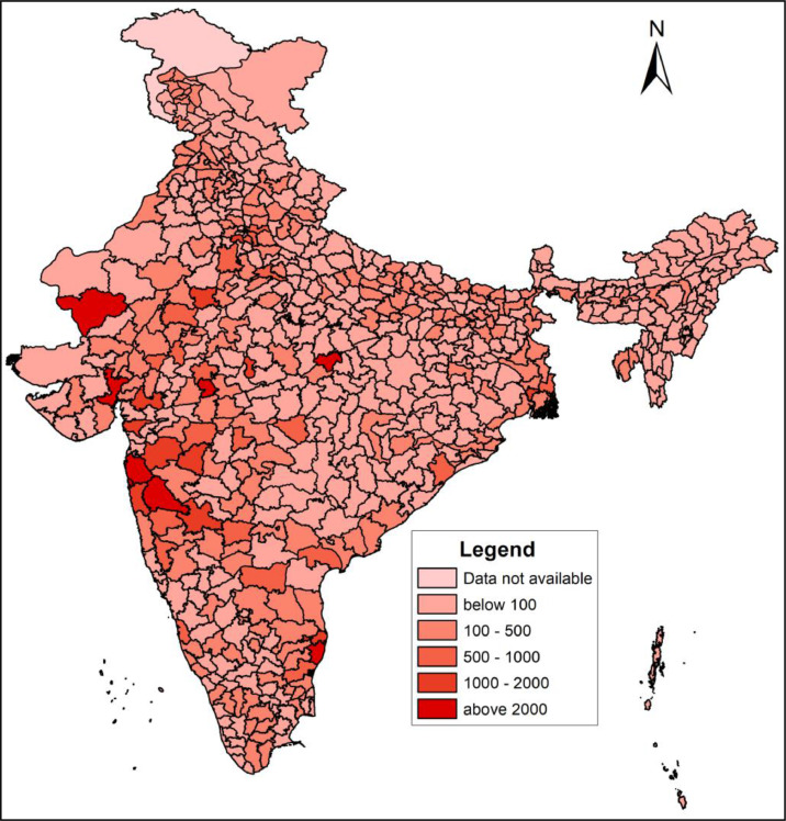
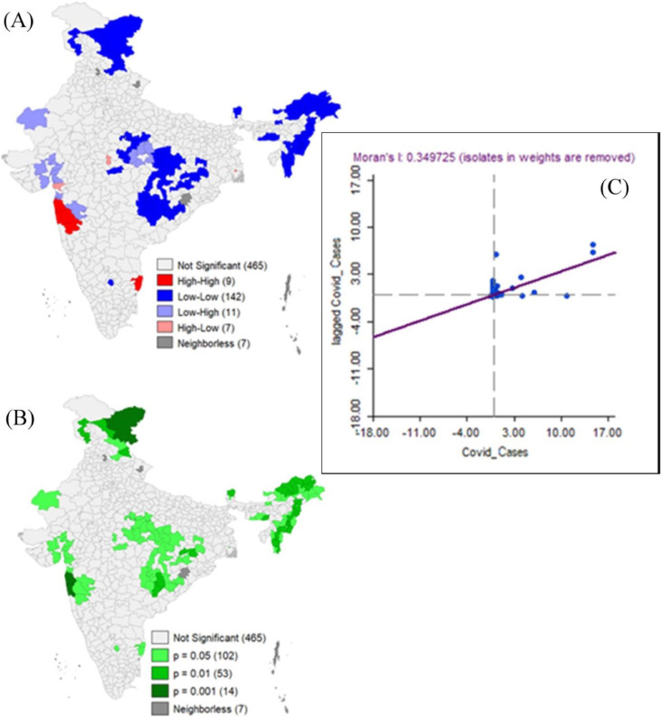
Spatial distribution of COVID-19 cases is presented in Fig. 2 . It is observed that the highest rates of COVID-19 cases are located in the western and southern parts of India. Significant autocorrelation can be observed from Fig. 3 (Moran's I= 0.35, p= 0.001), indicates that COVID-19 cases between the districts is highly spatially correlated.

Fig. 2.

Spatial distribution of COVID-19 cases (3^rd June, 2020)

Fig. 3.

Spatial Cluster map associated with COVID-19 cases by districts (3^rd June, 2020), A) Significant Clusters obtained through LISA, B) Significance Map and P-values associated with spatial cluster map, C) Scatter plot and Moran's I Value.

Fig. 3 shows significant clusters of COVID-19 cases. The cluster was delimited with four zones. High-high cluster with red colour indicates towards the district of Maharashtra, Tamilnadu and West Bengal with significant COVID-19 cases surrounded by similar cases. In contrast, lo-low cluster with blue colour is delimited with low COVID-19 cases surrounded by similar cases towards the districts of North-eastern states, Jammu and Kashmir, Madhya Pradesh, Chhattishgarh, Orissa (Fig. 3).

3.2. Summary statistics of variables for COVID-19 spread

After the selection and correlation analysis among the 19 selected variables, only three variables were selected to be included in the suitable model analysis. These are, households having bank facility, urbanization and population density. It is observed from Table 2 that, these selected variables have very low multi-collinearity as the VIFs value is less than the threshold value of 5 (less than 1.5) (Mollalo et al., 2020; O'brien, 2020).

Table 2.

Summary statistics for OLS model.

Variable	Coefficient	T-statistics	Sig.	VIF
CONSTANT	-428.30	-1.07	0.28	-
Bank facility	4.19	0.62	0.54	1.09
Urbanization	11.01	1.74	0.08	1.45
Population density	0.34	7.97	0.00	1.38

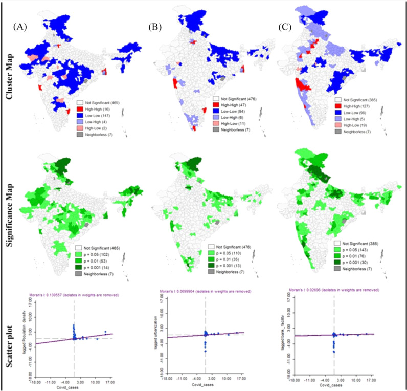
Maps for each significant variable with COVID-19 cases are presented in Fig. 4 . Bivariate LISA significant cluster was performed between each variable and COVID-19 case. A positive autocorrelation was observed between population density and COVID-19 rates (Moran's I= 0.13, p= 0.002). Districts with high population density and high COVID-19 cases are almost same with the areas with high-high and low-low COVID-19 clusters. There is a positive spatial correlation between urbanization and COVID-19 rates (Moran's I= 0.07, p= 0.001). The positive relationship between bank facility and COVID-19 cases is also confirmed (Moran's I= 0.03, p= 0.001). Both high-high and low-low clusters are almost same with the district of cluster for COVID-19 cases. This shows that inspite of having low Moran's I value, overall the variables are spatially correlated with COVID-19 rates indicates the direct association among them.

Fig. 4.

Bivariate LISA cluster and significant map between significant variable and COVID-19 cases, A) Population density, B) Urbanization in 2011, C) Households have banking facility.

3.3. Spatial modelling for COVID-19 rates

A suitable spatial model is necessary as OLS model has shown a very low adjusted R2. Low adjusted R2 of OLS implies that almost 85% of the COVID-19 cases across India are caused by unknown variables which are not captured by the model. Therefore this study confirmed the need for a spatial model to picture the COVID-19 incidents. Table 3 shows the summary statistics of spatial lag model (SLM) and spatial error model (SEM). These models show an improvement of performance than global OLS model in modelling the COVID-19 factors in India. In both cases autoregressive lag coefficients (i.e., ρ and λ) are strongly significant (p<0.000). Between these two models, lag model shows relatively low standard error than error model. However, both SLM and SEM models shows better performance than OLS, but still a poor performance regarding the framing of COVID-19 cases in India (Table 4 ). This result may be caused by the neglected scale at local level involved in modelling the COVID-19 incidence in India.

Table 3.

Summary Statistics for SLM and SEM models.

Variable	Coefficient		Std. Error		Z-Score		P-Value
	SLM	SEM	SLM	SEM	SLM	SEM	SLM	SEM
CONSTANT	-396.53	-749.83	374.04	526.71	-1.06	-1.42	0.29	0.15
Bank facility	3.23	9.50	6.36	8.60	0.51	1.10	0.61	0.27
Urbanization	5.92	8.51	5.93	6.49	1.00	1.31	0.32	0.19
Population density	0.33	0.44	0.04	0.04	7.97	10.23	0.00	0.00
LAMBDA	-	0.54	-	0.05	-	11.55	-	0.00
W_Covid case	0.44	-	0.05	-	8.92	-	0.00	-

Table 4.

Comparison of different models for goodness of fit in modelling COVID-19 rates.

Criterion	OLS	SEM	SLM	GWR	MGWR
Adj R2	0.15	0.30	0.25	0.74	0.75
AICc	11977.06	11887.36	11921.26	11253.73	963.90

To test the factor of scale in modelling the COVID-19 incidences, two local level regression model were employed namely GWR and MGWR. According to Table 4, adjusted R2 value increases significantly and it is 15% in OLS, 30% in SEM, 25% in SLM, 74% in GWR model and 75% in MGWR model. This numeric figure showed that MGWR can explain upto 75% of the variables that are causing the COVID-19 incidences in India. This fact is also supported by the dropping figure of AICc from 11977.06 for OLS to 963.90 for MGWR. This indicates that MGWR model is the most suitable model for modelling COVID-19 incidences with the highest R2 value and lowest AICc which is slightly higher than the regular GWR model.

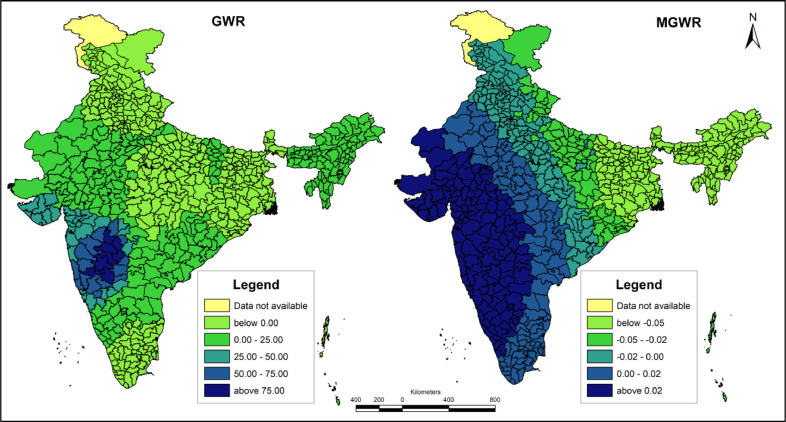
Figs. 4, 5 and 6 show the results of coefficients of GWR and MGWR for the selected variables. As observed form the Fig. 5, effect of population density demonstrates almost similar pattern describing the COVID-19 incidence in India at district level for both GWR and MGWR models. Population density is an important factor in influencing the COVID-19 rates across the country especially in the western parts like Gujarat, Maharashtra for both models.

Fig. 5.

Effects of population density in describing COVID-19 using GWR and MGWR.

Fig. 6.

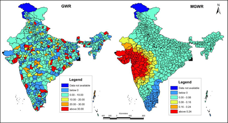
Effects of bank facility in describing COVID-19 using GWR and MGWR.

In Fig. 6 the impact of bank facility over COVID-19 incidences is inconsistent between GWR and MGWR models. However, it shows the similar kind of impact like the population density. The western part is showing high coefficients values than the north, eastern and north-eastern part of India.

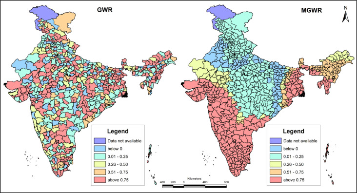
Fig. 7 describes the impact of urbanization on COVID-19 cases. This figure also shows the inconsistency between the impact in GWR and MGWR models. In GWR model, it is observed that there is not any general spatial pattern whereas the MGWR model reflects a similar spatial pattern like Figs. 4 and 5.

Fig. 7.

Effects of urbanization in describing COVID-19 using GWR and MGWR.

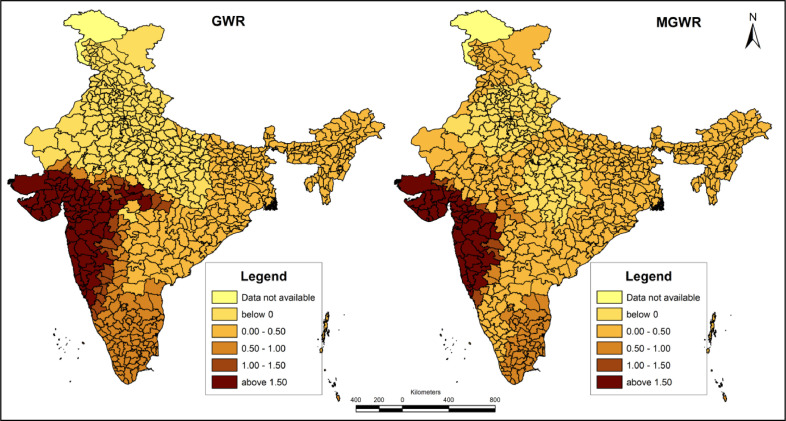
Fig. 8 shows the spatial distribution of local R2 values associated with population density, bank facility and urbanization in India in both GWR and MGWR model. In GWR model, it is observed that there is no significant general pattern of R2 distribution at local level. On the contrary, in MGWR, it is found that the district of Gujarat, Maharashtra, Karnataka, Kerala, Tamilnadu, Andhra Pradesh, West Bengal, Tripura, Mizoram had very high R2 value which indicates a very decent fit of the model in these areas. Although there is a clear difference between the goodness of fit of both GWR and MGWR model, it is found that MGWR model is most suitable for predicting the COVID-19 incidences in India.

Fig. 8.

Distribution of Local R² of GWR and MGWR.

4. Discussion

In this study, GIS based approach was adopted for modelling the COVID-19 incident and its vectors. 19 explanatory variables were considered that could potentially explain the pattern of COVID-19 outbreaks. These variables were broadly categorized under three groups, such as, adaptive, sensitivity and exposure. After analyzing the variables and removing the tendency of multi-collinearity, three important variables were considered for the further study namely population density, HHs (Households) having bank facility and rate of urbanization. Several statistical models had been used to model the incidence and the relationship with the explanatory variables. Among the models, MGWR was found to be the best model in explaining the factors of COVID-19 incidence rate.

The study demonstrates that urbanization rate shows a positive effect over COVID-19 cases. As a demographic process, it leads to an increase in human mobility and population density, which ultimately reduces the social distancing. Along with that, the level of pollution, overcrowding becomes also relevant for COVID-19 outbreaks. More importantly, this study shows that population density has the most significant effects over COVID-19 outbreaks. Findings of GWR and MGWR show a significant positive relationship between COVID-19 diseases and population density. Increasing population density facilitates spread of the disease at a very fast rate due to lower social distancing.

However, this study does not found any significant contribution of climatic phenomena over COVID-19 outbreaks. In their study over China, Ma et al., (2020) found positive integration between temperature range and COVID-19. The role of older adults also does not show any significant contribution in controlling COVID-19 diseases. In Iran, Ramírez-Aldana et al., (2020) found this factor as the most important factor having the maximum effect over COVID-19 outbreaks. They predicted that, 1% increase of older aging more than 60, can cause a multiplicative effect of 1490 COVID-19 cases.

However, this study has some limitations. The main limitation of this study was the data availability. Most of the data of the variables used as explanatory variables were backdated and not updated. Another limitation was, different states and union territories (UT) have their own perspective of policy making. Therefore, this generalised proposal of policy taking may cause extraordinary impacts on different cases. This study also does not include different pre-existing health issues such as, mental tension, cardiovascular conditions which are considered vulnerable to COVID-19. Incorporation of such risk factors may be helpful in influencing COVID-19 (Bansal, 2020; Saha and Chouhan, 2020). For example, it is observed that persons with pre-existing health issues are more susceptible and vulnerable to the Covid-19 (Mhango et al., 2020; Tahmasebi et al., 2020). Therefore, inclusion of the number of persons having co-morbidity may deliver slightly better output. Future studies may focus in improving the vectors that not only transmit disease but also relates transmission dynamics.

5. Conclusion

Despite all the limitations, this study approached a spatial statistical analysis that helps to identify district level variation of potential factors that facilitates COVID-19 disease. It may be also applicable for others countries with similar characteristics. This study considers multiple factors for the outbreak of this pandemic and could help to monitor the areas with high incidence rates. GWR and MGWR are very helpful in monitoring the relationship between COVID-19 and variables. The result confirmed that MGWR accomplished the highest goodness-of-fit among the other models. The performance of MGWR can vary over different nation in response to different variables. This study could be helpful for further research for modelling disease.

Declaration of Competing Interest

The authors certify that they have NO affiliations or involvement in any other organization or entity with any financial interest (such as honoraria; educational grants; participation in speakers’ bureaus; membership, employment, consultancies, stock ownership, or other equity interest; and expert testimony or patent-licensing arrangements), or non-financial interest (such as personal or professional relationships, affiliations, knowledge or beliefs) in the subject matter or materials discussed in this manuscript.

References

- Auler A.C., Cássaro F.A.M., da Silva V.O., Pires L.F. Evidence that high temperatures and intermediate relative humidity might favor the spread of COVID-19 in tropical climate: A case study for the most affected Brazilian cities. Sci. Total Environ. 2020 doi: 10.1016/j.scitotenv.2020.139090. [DOI] [PMC free article] [PubMed] [Google Scholar]
- Bansal M. Cardiovascular disease and COVID-19. Diab. Metab. Syndrome: Clin. Res. Rev. 2020;14(3):247–250. doi: 10.1016/j.dsx.2020.03.013. [DOI] [PMC free article] [PubMed] [Google Scholar]
- Bärnighausen T., Hosegood V., Timaeus I.M., Newell M.L. The socioeconomic determinants of HIV incidence: evidence from a longitudinal, population-based study in rural South Africa. AIDS (London, England) 2020;21(Suppl 7):S29. doi: 10.1097/01.aids.0000300533.59483.95. [DOI] [PMC free article] [PubMed] [Google Scholar]
- Bluhm R., Pinkovskiy M. The spread of COVID-19 and the BCG vaccine: A natural experiment in reunified Germany. FRB of New York Staff Report. 2020;(926) [Google Scholar]
- Das A., Ghosh S., Das K., Basu T., Das M., Dutta I. Modelling the Effect of Area-deprivation on COVID-19 Incidences: a study of Chennai Megacity. India. Public Health. 2020 doi: 10.1016/j.puhe.2020.06.011. [DOI] [PMC free article] [PubMed] [Google Scholar]
- Das A., Ghosh S., Das K., Dutta I., Basu T., Das M. (In) visible impact of inadequate WaSH Provision on COVID-19 incidences can be not be ignored in large and megacities of India. Public Health. 2020 doi: 10.1016/j.puhe.2020.05.035. [DOI] [PMC free article] [PubMed] [Google Scholar]
- Farr B.M., Bartlett C.L.R., Wadsworth J., Miller D.L., THE I.A.W.M.O., British Thoracic Society Pneumonia Study Group Risk factors for community-acquired pneumonia diagnosed upon hospital admission. Respir. Med. 2000;94(10):954–963. doi: 10.1053/rmed.2000.0865. [DOI] [PubMed] [Google Scholar]
- Gibson L., Rush D. Novel corona virus in Cape Town informal settlements: feasibility of using informal dwelling outlines to identify high risk areas for COVID-19 transmission from a social distancing perspective. JMIR Public Health Surveill. 2020;6(2):e18844. doi: 10.2196/18844. [DOI] [PMC free article] [PubMed] [Google Scholar]
- Gupta R., Ghosh A., Singh A.K., Misra A. Clinical considerations for patients with diabetes in times of COVID-19 epidemic. Diab. Metab. Syndrome. 2020;14(3):211–212. doi: 10.1016/j.dsx.2020.03.002. Advance online publication. [DOI] [PMC free article] [PubMed] [Google Scholar]
- Huang X., Lambert S., Lau C., Magalhaes R.S., Marquess J., Rajmokan M., Milinovich G., Hu W. Assessing the social and environmental determinants of pertussis epidemics in Queensland, Australia: a Bayesian spatio-temporal analysis. Epidemiol. Infect. 2017;145(6):1221–1230. doi: 10.1017/S0950268816003289. [DOI] [PMC free article] [PubMed] [Google Scholar]
- Kang J.Y., Michels A., Lyu F., Wang S., Agbodo N., Freeman V.L., Wang S. Rapidly measuring spatial accessibility of COVID-19 healthcare resources: a case study of Illinois, USA. Int. J. Health Geogr. 2020;19(1):1–17. doi: 10.1186/s12942-020-00229-x. [DOI] [PMC free article] [PubMed] [Google Scholar]
- Khalatbari-Soltani S., Cumming R.C., Delpierre C., Kelly-Irving M. Importance of collecting data on socioeconomic determinants from the early stage of the COVID-19 outbreak onwards. J. Epidemiol. Community Health. 2020;74(8):620–623. doi: 10.1136/jech-2020-214297. [DOI] [PMC free article] [PubMed] [Google Scholar]
- Lakhani A. Which Melbourne metropolitan areas are vulnerable to COVID-19based on age, disability and access to health services? Using spatial analysis to identify service gaps and inform delivery. J. Pain Symptom Manag. 2020;S0885-3924(20):30194–30199. doi: 10.1016/j.jpainsymman.2020.03.041. (Published online ahead of print) [DOI] [PMC free article] [PubMed] [Google Scholar]
- Lau H., Khosrawipour V., Kocbach P., Mikolajczyk A., Ichii H., Zacharksi M., Bania J., Khosrawipour T. The association between international and domestic air traffic and the coronavirus (COVID-19) outbreak. J. Microbiol. Immunol. Infect. 2020;53(3):467–472. doi: 10.1016/j.jmii.2020.03.026. [DOI] [PMC free article] [PubMed] [Google Scholar]
- Liu J., Zhou J., Yao J., Zhang X., Li L., Xu X., He X., Wang B., Fu S., Niu T., Yan J., Shi Y., Ren X., Niu J., Zhu W., Li S., Luo B., Zhang K. Impact of meteorological factors on the COVID-19 transmission: a multi-city study in China. Sci. Total Environ. 2020 doi: 10.1016/j.scitotenv.2020.138513. [DOI] [PMC free article] [PubMed] [Google Scholar]
- Ma Y., Zhao Y., Liu J., He X., Wang B., Fu S. Effects of Temperature Variation and Humidity on the Mortality of COVID-19 in Wuhan. medRxiv. 2020 doi: 10.1016/j.scitotenv.2020.138226. Google Scholar. [DOI] [PMC free article] [PubMed] [Google Scholar]
- Mhango M., Dzobo M., Chitungo I., Dzinamarira T. COVID-19 risk factors among health workers: a rapid review. Saf. Health at Work. 2020 doi: 10.1016/j.shaw.2020.06.001. [DOI] [PMC free article] [PubMed] [Google Scholar]
- Mollalo A., Vahedi B., Rivera K.M. GIS-based spatial modeling of COVID-19 incidence rate in the continental United States. Sci. Total Environ. 2020;728 doi: 10.1016/j.scitotenv.2020.138884. [DOI] [PMC free article] [PubMed] [Google Scholar]
- O'brien R.M. A caution regarding rules of thumb for variance inflation factors. Qual.Quant. 2020;41(5):673–690. [Google Scholar]
- Ramírez-Aldana R., Gomez-Verjan J.C., Bello-Chavolla O.Y. Spatial analysis of COVID-19 spread in Iran: Insights into geographical and structural transmission determinants at a province level. medRxiv. 2020 doi: 10.1371/journal.pntd.0008875. Google Scholar. [DOI] [PMC free article] [PubMed] [Google Scholar]
- Saha J., Chouhan P. Indoor air pollution (IAP) and pre-existing morbidities among under-5 children in India: are risk factors of coronavirus disease (COVID-19)? Environ. Pollut. 2020;266 doi: 10.1016/j.envpol.2020.115250. [DOI] [PMC free article] [PubMed] [Google Scholar]
- Taghizadeh-Hesary F., Akbari H. The powerful immune system against powerful COVID-19: a hypothesis. Med. Hypotheses. 2020;140 doi: 10.1016/j.mehy.2020.109762. [DOI] [PMC free article] [PubMed] [Google Scholar]
- Tahmasebi P., Shokri-Kuehni S.M., Sahimi M., Shokri N. How do environmental, economic and health factors influence regional vulnerability to COVID-19? MedRxiv. 2020 [Google Scholar]
- Tata Capitalblog. 2020. What are the Steps Taken by the Government to Fight Coronavirus in India? https://www.tatacapital.com/blog/trends/what-are-the-steps-taken-by-the-government-to-fight-coronavirus-in-india/. (accessed on June 4th, 2020).
- United Nations. Department of Economic and Social Affairs Social Inclusion. 2020. https://www.un.org/development/desa/dspd/2020/04/covid19-social-crisis/. (accessed on June 4th, 2020).
- Wang L., Li J., Guo S., Xie N., Yao L., Cao Y., Day S.W., Howard S.C., Graff J.C., Gu T., Ji J. Real-time estimation and prediction of mortality caused by COVID-19 with patient information based algorithm. Sci. Total Environ. 2020;727 doi: 10.1016/j.scitotenv.2020.138394. [DOI] [PMC free article] [PubMed] [Google Scholar]
- Ward M.D., Gleditsch K.S. Sage Publications; 2018. Spatial Regression Models (Vol. 155) [Google Scholar]
- Wu X., Nethery R.C., Sabath B.M., Braun D., Dominici F. Exposure to air pollution and COVID-19 mortality in the United States: A nationwide cross-sectional study. medRxiv. 2020 doi: 10.1126/sciadv.abd4049. [DOI] [PMC free article] [PubMed] [Google Scholar]
- Yongjiana Z., Jingubc X., Fengmingb H., Liqingb C. Association between short term exposure to air pollution and COVID-19 infection: evidence from China. Sci. Total Environ. 2020;727 doi: 10.1016/j.scitotenv.2020.138704. [DOI] [PMC free article] [PubMed] [Google Scholar]
- Zhu Y., Xie J. Association between ambient temperature and COVID-19 infection in 122 cities from China. Sci. Total Environ. 2020;724 doi: 10.1016/j.scitotenv.2020.138704. [DOI] [PMC free article] [PubMed] [Google Scholar]