On the necessity of proper quarantine without lock down for 2019-nCoV in the absence of vaccine

Abstract

Presently the world is passing through a critical phase due to the prevalence of the Novel Corona virus, 2019-nCoV or COVID-19, which has been declared a pandemic by WHO. The virus transmits via droplets of saliva or discharge from the nose when an infected person coughs or sneezes. Due to the absence of vaccine, to prevent the disease, social distancing and proper quarantine of infected populations are needed. Non-resident citizens coming from several countries need to be quarantined for 14 days prior to their entrance. The same is to be applied for inter-state movements within a country. The purpose of this article is to propose mathematical models, based on quarantine with no lock down, that describe the dynamics of transmission and spread of the disease thereby proposing an effective preventive measure in the absence of vaccine.

Introduction

Viruses are not new on Earth. Since the evolution of first living cells they existed as most numerous biological entity in almost ecosystem having infected all life forms besides human beings. The history of human race was disrupted several times by terrible impacts of viral infections. During last one year the entire world is facing challenges posed by novel corona virus 2019, commonly known as COVID-19 and the battle is not over yet. A new strain of COVID-19 has become very dangerous through its exceptional infectious qualities [3]. Reportedly, China country office of WHO, for the first time on December ${31}^{\mathit{st}}$,2019, come to know about cases of pneumonia of unknown aetiology which was detected in Wuhan city, Hubei Province of China. Up to January $3^{\mathit{rd}}$,2020, a total of 44 cases of pneumonia with unknown cases were reported. Subsequently on January $7^{\mathit{th}}$, 2020, it was identified that the pathogenic agent behind the cases of pneumonia was corona virus of a new strain. On January ${13}^{\mathit{th}}$, 2020, the first imported case of novel corona virus (2019-nCoV) was reported by the Ministry of Public Health, Thailand [9], [14], [21]. With the passage of time the whole world have been hit by the rapid spread of COVID-19. As reported by WHO [22] a total of 8385440 confirmed cases of COVID-19 positive and total of 450686 deaths have taken place by ${19}^{\mathit{th}}$ June,2020. The following table 1 shows a list of top 12 countries with respect to transmission of COVID-19.

Table 1.

World top 12 countries with reported laboratory-confirmed COVID-19 cases and deaths; data as of ${19}^{\mathit{th}}$ June, 2020 [22].

Country Name	Total confirmed cases	Total confirmed new cases	Total deaths	Total new deaths
United States of America	2149166	23139	117472	770
Brazil	955377	32188	46510	1269
Russian Federation	569063	7972	7841	181
India	380532	13586	12573	336
The United Kingdom	300473	1218	42288	135
Spain	245268	585	27136	0
Peru	240908	3752	7257	201
Italy	238159	331	34514	66
Chile	225103	4475	3841	226
Iran	197647	2596	9272	87
Germany	187764	0	8856	0
Turkey	184031	1304	4882	21

Way back in $1918-19$ the world had seen a pandemic of similar extent when the human civilization was attacked by H1N1 influenza. Since there was no vaccine available, different governments took different measures to contain the transmission of the virus in their countries.These pharmaceutical interventions (NPIs) included closing schools, churches, bars and other places of social gathering. The places where these interventions were implemented early were successful in reducing the number of cases while a lower mortality rate were experience in place where interventions remained in place. But with the lifting of controls the transmission renounced once again [10].

Now we, the whole human civilization over the globe, experience a very similar kind of situation in combating COVID-19 with so called non-pharmaceutical interventions which aims at reducing contact rates in the population to arrest the transmission of the virus [11], [24]. Such measures include the reduction of social contact in work places, schools and other public domains. For quantitative estimates of the impact of these measures in reducing morbidity, infection rate, excess mortality, proper mathematical model of virus transmission are required and these can contribute significantly in the public health planning.

To combat against COVID-19 the measures that included closing of international borders, shutting school, colleges and workplaces containing large gatherings (“Great lock down”, the phrase coined by the IMF), has invited huge impact on global economy which resulted in people to loose their jobs and businesses being disrupted. It’s truly a global crisis.

At this point of time mathematics has emerged to be an invaluable weapon to combat against COVID-19. Mathematical models allow public health officials to conduct virtual experiments thereby evaluating the efficacious of control strategies. By studying the transmission dynamics [15], [19] a systematic quarantine strategy can be taken up.

Epidemic outbreaks evolve in geographic territories with considerable variability in spatial footings. This spatial inconstancy is significant in understanding the dominance of public health policies and interventions in regulating these epidemics. A major trouble in provoking models to narrate spatial inconstancy in epidemics is accounting for the movement of people in spatial contexts. Multiple approaches to generate such statement have been exhibited, including individual based models, network models, stochastic models, and partial differential equations models. For the geographic spread [4] and control of COVID-19, we consider two epidemic models of partial differential equations [8], [17] corresponding to the epidemic 2019-nCoV, one is due to proper quarantine of infected population and other is due to no quarantine. To include and quantify spatial effect we consider these models as diffusion models [1], [5], [15] for the geographic spread of the epidemic. The problem we interested in including a number of E class and I class in a uniform population together with homogeneous initial susceptible volume $S_0$ and calculating geotemporal propagation of the malady. Nomenclatures used in the epidemic models of the pandemic disease COVID-19 is given in the Table 2 .

Table 2.

Nomenclature for the models.

Symbols	Descriptions
$S(x,t)$	Susceptible population
$E(x,t)$	A population in which the disease is latent
$I(x,t)$	Infected population
$R(x,t)$	Removed population
${\lambda }_1$	Rate of contact between S and E class
${\lambda }_2$	Rate of contact between S and I class
${\lambda }_3$	A fraction of ${\lambda }_1$ that belong to E class
${\lambda }_4$	Rate of contact between E and I class
${\lambda }_5$	A fraction of ${\lambda }_1$ that belong to I class
$\gamma$	Rate at which both E and I classes release their individuals from their respective classes
D	Diffusion coefficient

Basic terminologies:

Susceptible population $S(x,t)$ : A susceptible population $S(x,t)$ in an epidemiology is a population at $x\in \mathrm{\Omega }\subset {\mathbb{R}}^n$ in time t, in which an infectious disease is not present but each individuals of this population is at risk of gaining infection by the disease in forward time.

Latent infected population $E(x,t)$ : A latent infected population $E(x,t)$ in an epidemiology is a population at $x\in \mathrm{\Omega }\subset {\mathbb{R}}^n$ in time t, in which an infectious disease (COVID-19 in our case) is present without any symptoms. In forward time they may belong to the infected population with symptoms or may become susceptible. They have ability to transmit the disease.

Infected population $I(x,t)$ :An infected population $I(x,t)$ in an epidemiology is a population at $x\in \mathrm{\Omega }\subset {\mathbb{R}}^n$ in time t, in which an infectious disease (COVID-19 in our case) is present with symptoms. In forward time they have full ability to transmit the disease through migrant population transmission or by local individual transmission or community transmission.

Removed population $R(x,t)$ : A removed population $R(x,t)$ in an epidemiology is a population at $x\in \mathrm{\Omega }\subset {\mathbb{R}}^n$ in time t, whose members are recovered from the infection of the infectious disease or died due to the infectious disease (COVID-19 in our case).

Basic reproduction rate $R_0$ : For an infectious disease (COVID-19 in our case) the basic reproductive number is the number of secondary infections delivered by a single infected individual in whole susceptible population. This quantity indicates the initial growth rate for the infected class and the potential for a large-scale epidemic. It is one of the touchstones of epidemiology.

Herd immunity: The immunization of an individual not only protects that individual but also indirectly protects others against the possibility of disease transmission from the immunized individual. If a sufficient fraction of a population is immunized, then an epidemic may be averted altogether. The protection of an entire population via the immunity of a fraction of the population is called herd immunity.

Epidemic models

In this section we develop two non-linear epidemic models [12], one is due to proper quarantine of infected population and other is due to no quarantine.

Hypothesis

For the non-linear epidemic model [12] the whole population N is considered to be constant. Due to diffusion, we consider the spread of the infection within the population as a function of time and space both. Let $\mathrm{\Omega }\subset {\mathbb{R}}^n$, be a bounded domain. Suppose the disease is such that the population can be separated into four distinct classes: the susceptible population, $S(x,t)$, who can grab the disease; the infected population, $I(x,t)$, who have the disease and can emit it; a class in which the disease is latent, $E(x,t)$, who also can transmit the disease; and the removed population, $R(x,t)$, namely, those who are recovered, immune or isolated until recovered or dies out; at the location $x\in \mathrm{\Omega }$ and at time t. Then

$$S+E+I+R=N,$$ (1)

Also suppose that ${\lambda }_1$ is the rate at which the interaction between the S class and the E class occur, ${\lambda }_2$ is the rate at which the interaction between the S class and the I class occur, ${\lambda }_3$ be the fraction of ${\lambda }_1$ for which the interaction between S class and E class belong to the E class, ${\lambda }_4$ is the rate at which the interaction between the I class and the E class occur, ${\lambda }_5$ be the remaining fraction of ${\lambda }_1$ for which the interaction between S class and E class belong to the I class, that is ${\lambda }_3+{\lambda }_5={\lambda }_1,\gamma$ be the rate at which both E class and I class release the individuals from their respective classes(in this case we choose the same rate for both E and I class) and D be the diffusion coefficient for all the population.

Model for no quarantine case

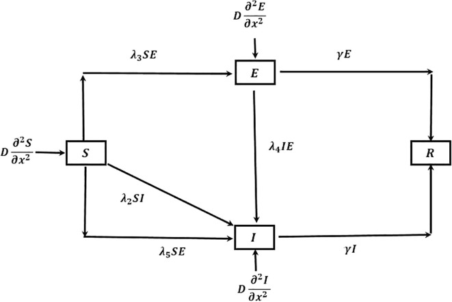
If there are no quarantine for infected populations, no social distancing and not considering for citizens of several countries that needed to be quarantined for 14 days earlier to entering their topical countries or topical state who comes outside their own country or own state respectively, the population of all $S,E$ and I classes are interact with each other. For which as time goes,the total populations has high probability to become latent infected as well as infected and the corresponding model is followed by the flow chart Fig. 1 , given by:

$$\frac{\partial S}{\partial t}=-({\lambda }_1\mathit{SE}+{\lambda }_2\mathit{SI})+D\frac{{\partial }^{2}S}{\partial x^2},$$ (2)

$$\frac{\partial E}{\partial t}={\lambda }_3\mathit{SE}-{\lambda }_4\mathit{IE}-\gamma E+D\frac{{\partial }^{2}E}{\partial x^2},$$ (3)

$$\frac{\partial I}{\partial t}={\lambda }_2\mathit{SI}+{\lambda }_4\mathit{IE}+{\lambda }_5\mathit{SE}-\gamma I+D\frac{{\partial }^{2}I}{\partial x^2}\text{.}$$ (4)

$$\frac{\partial R}{\partial t}=\gamma (I+E)\text{.}$$ (5)

Fig. 1.

Flow of COVID-19 transmission for ‘no quarantine case’.

It is easy to check that the system (2), (4) has infinitely many solutions. The following results show that the solutions of the system (2), (4) are non-negative and uniformly bounded. First we represent a non-negativity lemma, which can be found in any standard book.

Lemma 1

Let $u\in C^{2,1}\left(\bar{\mathrm{\Omega }}\times [0,\tau ]\right)\cap C^{2,1}\left(\mathrm{\Omega }\times [0,\tau ]\right)$ with

$$u_t-D\mathrm{\Delta }u⩾a(x,t)u\text{;}x\in \mathrm{\Omega },0<t⩽\tau$$

$$\frac{\partial u}{\partial \eta }⩾0\text{;}x\in \partial \mathrm{\Omega },0<t⩽\tau$$

$$u(x,0)⩾0\text{;}x\in \bar{\mathrm{\Omega }}$$

where $a(x,t)\in C^{2,1}\left(\bar{\mathrm{\Omega }}\times [0,\tau ]\right)$ and $\frac{\partial u}{\partial \eta }$ is the outward normal derivative of u at $\partial \mathrm{\Omega }$ . Then $u(x,t)⩾0$ on $\bar{\mathrm{\Omega }}\times [0,\tau ]$ . Moreover $u(x,t)>0$ or $u(x,t)=0$ in $\mathrm{\Omega }\times [0,\tau ]$ .

Proposition 1

For a non-negative initial condition, the system (2), (4) possesses a non-negative solution.

Proof

Let $\left(S,E,I\right)$be a solution of the system (2), (4) in $\mathrm{\Omega }\times [0,T_{\mathit{max}}]$. Then for every $\tau \in \left(0,T_{\mathit{max}}\right)$and from the system (2), (4)

$$S_t-D\mathrm{\Delta }S=-\left({\lambda }_{1}E+{\lambda }_{2}I\right)S$$

$$E_t-D\mathrm{\Delta }E=\left({\lambda }_{3}S-{\lambda }_{4}I-\gamma \right)E$$

$$I_t-D\mathrm{\Delta }I={\lambda }_2\mathit{SI}+{\lambda }_4\mathit{IE}+{\lambda }_5\mathit{SE}-\gamma I⩾\left({\lambda }_{2}S+{\lambda }_{4}E-\gamma \right)I$$

where $x\in \mathrm{\Omega },0<t⩽\tau$. Also ${\lambda }_{1}E+{\lambda }_{2}I,{\lambda }_{3}S-{\lambda }_{4}I-\gamma$and ${\lambda }_{2}S+{\lambda }_{4}E-\gamma$ are bounded in $\mathrm{\Omega }\times [0,\tau ]$.

Thus from Lemma (1, as $\tau$ is arbitrary in $\left(0,T_{\mathit{max}}\right)$, we must have $S(x,t)⩾0,E(x,t)⩾0$ and $I(x,t)⩾0$ in $\mathrm{\Omega }\times [0,\tau ]$. Hence the proof. □

Proposition 2

For a non-trivia and non-negative initial value let $\left(S,E,I\right)\in {\left[\in C^{2,1}\left(\bar{\mathrm{\Omega }}\times [0,T_{\mathit{max}})\right)\cap C^{2,1}\left(\mathrm{\Omega }\times (0,T_{\mathit{max}})\right)\right]}^3$ be a solution of the system (2), (4) . Then $T_{\mathit{max}}=\infty$ and

$0<S(x,t)+E(x,t)+I(x,t)⩽\mathit{max}\{{\left|\left|S_0\left(x\right)+E_0\left(x\right)+I_0\left(x\right)\right|\right|}_{\infty }+{\left|\left|S_0^{\prime }\left(x\right)+E_0^{\prime }\left(x\right)+I_0^{\prime }\left(x\right)\right|\right|}_{\infty }+{\left|\left|S_0^{″}\left(x\right)+E_0^{″}\left(x\right)+I_0^{″}\left(x\right)\right|\right|}_{\infty },N\}$ , where prime denote the differentiation with respect to x and N is given by the relation (1) .

Proof

First we show that all of $S(x,t),E(x,t)$ and $I(x,t)$ are bounded in $\mathrm{\Omega }\times (0,T_{\mathit{max}})$. Let $U(x,t)=S(x,t)+E(x,t)+I(x,t)$. As.

$0<U(x,0)⩽{\left|\left|U_0\left(x\right)\right|\right|}_{\infty }+{\left|\left|U_0^{\prime }\left(x\right)\right|\right|}_{\infty }++{\left|\left|U_0^{″}\left(x\right)\right|\right|}_{\infty }$ and

$${\left(S+E+I\right)}_t-D\mathrm{\Delta }\left(S+E+I\right)=-\gamma \left(E+I\right)⩽\gamma N-\gamma \left(S+E+I\right),$$

we must have $0<U(x,0)⩽w\left(t\right)$ in $\mathrm{\Omega }\times (0,T_{\mathit{max}})$, where

$w\left(t\right)=\left[N+\left({\left|\left|U_0\left(x\right)\right|\right|}_{\infty }+{\left|\left|U_0^{\prime }\left(x\right)\right|\right|}_{\infty }+{\left|\left|U_0^{″}\left(x\right)\right|\right|}_{\infty }-N\right)e^{-\gamma t}\right]$for $t\in [0,\infty )$ is the solution of the ODE

$$\frac{\mathit{dw}\left(t\right)}{\mathit{dt}}=\gamma N-\gamma w\left(t\right),$$

$w\left(0\right)={\left|\left|U_0\left(x\right)\right|\right|}_{\infty }+{\left|\left|U_0^{\prime }\left(x\right)\right|\right|}_{\infty }+{\left|\left|U_0^{″}\left(x\right)\right|\right|}_{\infty }$.

Thus we have $0<w\left(t\right)⩽\mathit{max}\left\{{\left|\left|U_0\left(x\right)\right|\right|}_{\infty }+{\left|\left|U_0^{\prime }\left(x\right)\right|\right|}_{\infty }++{\left|\left|U_0^{″}\left(x\right)\right|\right|}_{\infty },N\right\}$ for $t\in [0,\infty )$.

Therefore $0<S(x,0)+E(x,0)+I(x,0)⩽w\left(t\right)$.

$⩽\mathit{max}\{{\left|\left|S_0\left(x\right)+E_0\left(x\right)+I_0\left(x\right)\right|\right|}_{\infty }+{\left|\left|S_0^{\prime }\left(x\right)+E_0^{\prime }\left(x\right)+I_0^{\prime }\left(x\right)\right|\right|}_{\infty }$

$+{\left|\left|S_0^{\prime }\left(x\right)+E_0^{\prime }\left(x\right)+I_0^{\prime }\left(x\right)\right|\right|}_{\infty }+{\left|\left|S_0^{″}\left(x\right)+E_0^{″}\left(x\right)+I_0^{″}\left(x\right)\right|\right|}_{\infty },N\}$. Hence the proof.

$R_0$ and Herd immunity for ‘no quarantine case’: For the reproductive rate of COVID-19 [23], [25], in the model (2), (5), considering initially $E_0=I_0$ the per capita increase of E and I class is given by

$$\frac{1}{\left(E+I\right)}\frac{\partial \left(E+I\right)}{\partial t}=\frac{\left({\lambda }_{1}E+{\lambda }_{2}I\right)S}{\left(E+I\right)}-\gamma \text{.}$$

Which gives us the basic reproductive rate

$$R_0=\frac{({\lambda }_1+{\lambda }_2)S_0}{\gamma }\text{.}$$

If $R_0>1$, then every infected member of the population will emit the disease to leastwise one other member during the infectious epoch, and the model argue that the disease will propagate within the population. If not, then the disease is desired to fall through before overreaching a substantive fraction of total population. Therefore $R_0=1$ is a critical epidemiological grade. In other terms, pathogens with elevated equilibrium of contagion and subordinate rescue and mortality rates will gesture an ideal threat. The reciprocal of the removal rate is the average time interval during which an individual from both E and I class remain contagious, given by $\frac{1}{\gamma }$.

The expression for $R_0$ can be rearranged to find the minimum size of a susceptible population, necessary for an epidemic to occur. Assuming that $R_0=1$, the threshold condition is given by

$$S_T=\frac{\gamma }{\left({\lambda }_1+{\lambda }_2\right)}\text{.}$$

A pathogen will go extinct if the size of the susceptible population is less than this threshold ($S<S_T$). If the population size is above this threshold, then we can rewrite the basic reproductive rate as

$$R_0=\frac{S_0}{S_T}\text{.}$$

Immunization reduces the size of the S class and thus leads to a smaller basic reproductive rate of the pathogen. In particular, immunizing a fraction p of a population reduces $R_0$ to

$$R_0^i=\frac{(1-p)S_0}{S_T}=(1-p)R_0\text{.}$$

Immunization will successfully eradicate the disease if it causes the basic reproductive rate to drop below one. Thus the critical immunization rate $p_c$ is

$$p_c=1-\frac{1}{R_0}\text{.}$$

Expansion of this model have been utilized to anticipate the necessity of minimum coverage to urge some other tangible diseases to mitigation. For example, measles and whooping cough two of the most contagious diseases are thought to require 90–95% coverage, chicken pox and mumps 85–90% coverage, polio and scarlet fever 82–97% coverage, and smallpox 70–80% coverage [2]. □

Re-parametrisation

For non-dimensionalisation, re-scaling dependent variables $S,E,I,R$ by $S_0$, the initial susceptible population and independent variables as $x,t$ by $x_0$ and $t_0$ respectively, let $S=S_0{S}^{\ast },E=S_0{E}^{\ast },I=S_0{I}^{\ast },R=S_0{R}^{\ast },t=t_0{t}^{\ast },x=x_0{x}^{\ast }$, where $S_0,t_0$ and $x_0$ are the characteristic units used to scale the above variables. Putting these in the system (2), (5) we get

$$\frac{S_0}{t_0}\frac{\partial S^{\ast }}{\partial t^{\ast }}=-\left({\lambda }_1{S}_0{S}^{\ast }{S}_0{E}^{\ast }+{\lambda }_2{S}_0{S}^{\ast }{S}_0{I}^{\ast }\right)+D\frac{S_0}{x_0^2}\frac{{\partial }^2{S}^{\ast }}{\partial x^{*2}}$$

$$\frac{S_0}{t_0}\frac{\partial E^{\ast }}{\partial t^{\ast }}={\lambda }_3{S}_0{S}^{\ast }{S}_0{E}^{\ast }-{\lambda }_4{S}_0{I}^{\ast }{S}_0{E}^{\ast }-\gamma S_0{E}^{\ast }+D\frac{S_0}{x_0^2}\frac{{\partial }^2{E}^{\ast }}{\partial x^{*2}}$$

$$\frac{S_0}{t_0}\frac{\partial I^{\ast }}{\partial t^{\ast }}={\lambda }_2{S}_0{S}^{\ast }{S}_0{I}^{\ast }+{\lambda }_4{S}_0{I}^{\ast }{S}_0{E}^{\ast }+{\lambda }_5{S}_0{S}^{\ast }{S}_0{E}^{\ast }-\gamma S_0{I}^{\ast }+D\frac{S_0}{x_0^2}\frac{{\partial }^2{I}^{\ast }}{\partial x^{*2}}$$

$$\frac{S_0}{t_0}\frac{\partial R^{\ast }}{\partial t^{\ast }}=\gamma S_0(I^{\ast }+E^{\ast })$$

that is,

$$\frac{\partial S^{\ast }}{\partial t^{\ast }}=-\left({\lambda }_1{t}_0{S}^{\ast }{S}_0{E}^{\ast }+{\lambda }_2{t}_0{S}^{\ast }{S}_0{I}^{\ast }\right)+D\frac{t_0}{x_0^2}\frac{{\partial }^2{S}^{\ast }}{\partial x^{*2}}$$

$$\frac{\partial E^{\ast }}{\partial t^{\ast }}={\lambda }_3{t}_0{S}^{\ast }{S}_0{E}^{\ast }-{\lambda }_4{t}_0{I}^{\ast }{S}_0{E}^{\ast }-\gamma t_0{E}^{\ast }+D\frac{t_0}{x_0^2}\frac{{\partial }^2{E}^{\ast }}{\partial x^{*2}}$$

$$\frac{\partial I^{\ast }}{\partial t^{\ast }}={\lambda }_2{t}_0{S}^{\ast }{S}_0{I}^{\ast }+{\lambda }_4{t}_0{I}^{\ast }{S}_0{E}^{\ast }+{\lambda }_5{t}_0{S}^{\ast }{S}_0{E}^{\ast }-\gamma t_0{I}^{\ast }+D\frac{t_0}{x_0^2}\frac{{\partial }^2{I}^{\ast }}{\partial x^{*2}}$$

$$\frac{\partial R^{\ast }}{\partial t^{\ast }}=\gamma t_0(I^{\ast }+E^{\ast })$$

With $S^{\ast }(x,0)=1,E^{\ast }(x,0)=\frac{E_0}{S_0},I^{\ast }(x,0)=\frac{I_0}{S_0},R^{\ast }(x,0)=0$ as initial conditions, where $E_0$ and $I_0$ are respectively the initial population of E and I class.

Letting $\gamma t_0=1$ and $D\frac{t_0}{x_0^2}=1$, we get $t_0=\frac{1}{\gamma }$ and $x_0={\left(\frac{D}{\gamma }\right)}^{\frac{1}{2}}$. Thus we end up with the scaled model

$$\frac{\partial S^{\ast }}{\partial t^{\ast }}=-{\mathit{aS}}^{\ast }{E}^{\ast }-(R_0-a)S^{\ast }{I}^{\ast }+\frac{{\partial }^2{S}^{\ast }}{\partial x^{*2}},$$ (6)

$$\frac{\partial E^{\ast }}{\partial t^{\ast }}={\mathit{bS}}^{\ast }{E}^{\ast }-\mu I^{\ast }{E}^{\ast }-E^{\ast }+\frac{{\partial }^2{E}^{\ast }}{\partial x^{*2}},$$ (7)

$$\frac{\partial I^{\ast }}{\partial t^{\ast }}=(R_0-a)S^{\ast }{I}^{\ast }+\mu I^{\ast }{E}^{\ast }+(a-b)S^{\ast }{E}^{\ast }-I^{\ast }+\frac{{\partial }^2{I}^{\ast }}{\partial x^{*2}}\text{.}$$ (8)

$$\frac{\partial R^{\ast }}{\partial t^{\ast }}=I^{\ast }+E^{\ast }\text{.}$$ (9)

with $S^{\ast }(x,0)=1,E^{\ast }(x,0)=\frac{E_0}{S_0}$ , $I^{\ast }(x,0)=\frac{I_0}{S_0},R^{\ast }(x,0)=0$ and four dimensionless numbers $a,b,\mu$ and $R_0$ as $a=\frac{{\lambda }_1{S}_0}{\gamma },b=\frac{{\lambda }_3{S}_0}{\gamma },\mu =\frac{{\lambda }_4{S}_0}{\gamma }$ and $R_0=\frac{({\lambda }_1+{\lambda }_2)S_0}{\gamma }$ respectively.

The parameters ${\lambda }_1$, …, ${\lambda }_5,\gamma$ and D in the dimensional model have been reduced to four dimensionless grouping $R_0,a,b$ and $\mu$.

Method of solution

In this model we investigate the local spread of an epidemic wave [13] of infection into a uniform susceptible population. We want to designate conditions for the existence of such travelling wave, its speed of propagation and, when it exists.

Looking for the one dimensional travelling wave solutions, let.

$S^{\ast }(x^{\ast },t^{\ast })=S^{\ast }\left(z\right),E^{\ast }(x^{\ast },t^{\ast })=E^{\ast }\left(z\right),I^{\ast }(x^{\ast },t^{\ast })=I^{\ast }\left(z\right),R^{\ast }(x^{\ast },t^{\ast })=R^{\ast }\left(z\right),z=x^{\ast }-{\mathit{ct}}^{\ast }$where the wave speed c, have to determine. The above consideration will gives us a travelling wave of constant shape in the direction of positive $x^{\ast }$-axis. Substituting the above consideration into the system (6), (9) we get the system of equations as

$$-c\frac{{\mathit{dS}}^{\ast }}{\mathit{dz}}=-{\mathit{aS}}^{\ast }{E}^{\ast }-(R_0-a)S^{\ast }{I}^{\ast }$$

$$-c\frac{{\mathit{dE}}^{\ast }}{\mathit{dz}}={\mathit{bS}}^{\ast }{E}^{\ast }-\mu I^{\ast }{E}^{\ast }-E^{\ast }$$

$$-c\frac{{\mathit{dI}}^{\ast }}{\mathit{dz}}=(R_0-a)S^{\ast }{I}^{\ast }+\mu I^{\ast }{E}^{\ast }+(a-b)S^{\ast }{E}^{\ast }-I^{\ast }$$

$$-c\frac{{\mathit{dR}}^{\ast }}{\mathit{dz}}=I^{\ast }+E^{\ast }$$

Which can be represented as

$$S^{\ast ″}+{\mathit{cS}}^{\ast \prime }-{\mathit{aS}}^{\ast }{E}^{\ast }-(R_0-a)S^{\ast }{I}^{\ast }=0,$$ (10)

$$E^{\ast ″}+{\mathit{cE}}^{\ast \prime }+{\mathit{bS}}^{\ast }{E}^{\ast }-\mu I^{\ast }{E}^{\ast }-E^{\ast }=0,$$ (11)

$$I^{\ast ″}+{\mathit{cI}}^{\ast \prime }+(R_0-a)S^{\ast }{I}^{\ast }+\mu I^{\ast }{E}^{\ast }+(a-b)S^{\ast }{E}^{\ast }-I^{\ast }=0\text{.}$$ (12)

$${\mathit{cR}}^{\ast \prime }+(I^{\ast }+E^{\ast })=0\text{.}$$ (13)

where prime represents differentiation w.r.t. z. The above system consists of finding range of parameters considered above, for which there exists a solution with positive wave speed c and non-negative $S^{\ast },I^{\ast }$ such that

$E^{\ast }(-\infty )=E^{\ast }\left(\infty \right)=0,S^{\ast }(-\infty )=1,S^{\ast }\left(\infty \right)=0,0⩽I^{\ast }(-\infty )<I^{\ast }\left(\infty \right)=1$

The conditions on $E^{\ast }$ and $I^{\ast }$ imply a pulse wave of infective population which propagates into the uninfected population. As time goes, the equations (11), (12) changes by linearising, with $S^{\ast }\to E^{\ast },E^{\ast }\to I^{\ast }$ and $I^{\ast }\to 1$ to get

$$S^{\ast ″}+{\mathit{cS}}^{\ast \prime }-R_0{S}^{\ast }\approx 0,$$ (14)

$$E^{\ast ″}+{\mathit{cE}}^{\ast \prime }+(b-\mu -1)E^{\ast }\approx 0,$$ (15)

$$I^{\ast ″}+{\mathit{cI}}^{\ast \prime }+(R_0+\mu -b-1)I^{\ast }\approx 0\text{.}$$ (16)

Phase plane analysis: From equation (15) a typical wave front solution is where $E^{\ast }$ towards one side, say, as $z\to -\infty$, is at one steady state and as $z\to \infty$ it is at the other. In that case we have to determine the value or values of c, for which the equation (15) has a non-negative solution $E^{\ast }$ which satisfies.

${\lim }_{z\to -\infty }{E}^{\ast }\left(z\right)=1,{\lim }_{z\to \infty }{E}^{\ast }\left(z\right)=0$.

In $(E^{\ast },U)$ phase plane.

$E^{\ast \prime }=U,U^{\prime }=-\mathit{cU}-(b-\mu -1)E^{\ast }$we have the phase plane trajectories as the solution of

$\frac{\mathit{dU}}{{\mathit{dE}}^{\ast }}=\frac{-\mathit{cU}-(b-\mu -1)E^{\ast }}{U}$which has one singular point for $(E^{\ast },U)$ as $(0,0)$. Corresponding to this singular point we define the matrix

$$A=\left(\begin{array}{cc}\hfill -c\hfill & \hfill -(b-\mu -1)\hfill \\ \hfill 1\hfill & \hfill 0\hfill \\ \hfill \hfill \end{array}\right)$$

whose eigenvalues are

$\frac{1}{2}\left[-c\pm \sqrt{c^2-4(b-\mu -1)}\right]$   $\Rightarrow$ $\left\{\begin{array}{cc}\hfill \mathit{stable}\mathit{node},\hfill & \hfill \mathit{if}{c}^2>4(b-\mu -1)\hfill \\ \hfill \mathit{stable}\mathit{spiral},\hfill & \hfill \mathit{if}{c}^2<4(b-\mu -1)\hfill \\ \hfill \hfill \end{array}\right)$ If $c⩾c_{\mathit{min}}=2\sqrt{b-\mu -1}$ then the singular point $(0,0)$ is a stable node. The case when $c=c_{\mathit{min}}$ gives us a degenerate node. If $c^2<4(b-\mu -1)$, it is a stable spiral; i.e., $E^{\ast }$ oscillates in a neighbourhood of the origin. By continuity disputes, in dimensional terms the range of c must satisfy

$$c⩾c_{\mathit{min}}=2\sqrt{b-\mu -1}=2\sqrt{\frac{{\lambda }_3{S}_0}{\gamma }-\frac{{\lambda }_4{S}_0}{\gamma }-1},\mu <b-1\text{.}$$

No wave solution exists for $\mu >b-1$. So this condition is necessary for the spread of epidemic wave for $E^{\ast }$ class.

There are a typical travelling wave solution when $c⩽2\sqrt{b-\mu -1}$. As $E^{\ast }<0$ for some z, they are physically unrealistic, because in that case $E^{\ast }$ spirals around the origin. In this seance $E^{\ast }\to 0$ at the leading edge with decreasing oscillation around $E^{\ast }=0$.

From equation (16) a typical wave front solution is where $I^{\ast }$ at one side, say, as $z\to \infty$, is at one steady state and as $z\to -\infty$ it is at the other. In that case we have to determine the value or values of c for which the equation (16) has a non-negative solution $I^{\ast }$ which satisfies.

${\lim }_{z\to -\infty }{I}^{\ast }\left(z\right)=1,{\lim }_{z\to \infty }{I}^{\ast }\left(z\right)=0$.

In $(I^{\ast },U)$ phase plane.

$I^{\ast \prime }=V,V^{\prime }=-\mathit{cV}-(R_0+\mu -b-1)I^{\ast }$we have the phase plane trajectories as solution of

$\frac{\mathit{dV}}{{\mathit{dI}}^{\ast }}=\frac{-\mathit{cV}-(R_0+\mu -b-1)I^{\ast }}{V}$which has one singular point for $(I^{\ast },V)$ as $(0,0)$. Corresponding to this singular point we define the matrix

$$A=\left(\begin{array}{cc}\hfill -c\hfill & \hfill -(R_0+\mu -b-1)\hfill \\ \hfill 1\hfill & \hfill 0\hfill \\ \hfill \hfill \end{array}\right)$$

whose eigenvalues are

$\frac{1}{2}\left[-c\pm \sqrt{c^2-4(R_0+\mu -b-1)}\right]$   $\Rightarrow$ $\left\{\begin{array}{cc}\hfill \mathit{stable}\mathit{node},\hfill & \hfill \mathit{if}{c}^2>4(R_0+\mu -b-1)\hfill \\ \hfill \mathit{stable}\mathit{spiral},\hfill & \hfill \mathit{if}{c}^2<4(R_0+\mu -b-1)\hfill \\ \hfill \hfill \end{array}\right)$ If $c⩾c_{\mathit{min}}=2\sqrt{R_0+\mu -b-1}$ then the singular point $(0,0)$ is a stable node. The case when $c=c_{\mathit{min}}$ gives us a degenerate node. If $c^2<4(R_0+\mu -b-1)$, it is a stable spiral; i.e., $I^{\ast }$ oscillates in a neighbourhood of the origin. By continuity disputes, in dimensional terms the range of c must satisfy.

$c⩾c_{\mathit{min}}=2\sqrt{R_0+\mu -b-1}=2\sqrt{\frac{(-{\lambda }_1+{\lambda }_2+{\lambda }_3+{\lambda }_4)S_0}{\gamma }-1}$,

$\mu >b+1-R_0$.

No wave solution exists for $\mu <b+1-R_0$. So this condition is necessary for $I^{\ast }$ class to propagate an epidemic wave.

There are a typical travelling wave solution when $c⩽2\sqrt{R_0+\mu -b-1}$. As $I^{\ast }<0$ for some z, they are physically unrealistic, because in that case $I^{\ast }$ spirals around the origin. In this seance $I^{\ast }\to 0$ at the leading edge with decreasing oscillation around $I^{\ast }=0$.

Analysis of analytical solution

Now solutions of equations (15), (16) are respectively given by

$$E^{\ast }\left(z\right)\propto \mathit{exp}\left[\frac{(-c\pm {\{c^2-4(b-\mu -1\left)\right\}}^{\frac{1}{2}})z}{2}\right],$$ (17)

and

$$I^{\ast }\left(z\right)\propto \mathit{exp}\left[\frac{(-c\pm {\{c^2-4(R_0+\mu -b-1\left)\right\}}^{\frac{1}{2}})z}{2}\right]\text{.}$$ (18)

As we required $E^{\ast }\left(z\right)\to I^{\ast }\left(z\right)$ and $I^{\ast }\left(z\right)\to 1$ with $E^{\ast }\left(z\right)>0$ and $I^{\ast }\left(z\right)>0$, these solutions can not oscillate about $E^{\ast }=I^{\ast }$ and $I^{\ast }=1$ respectively; otherwise $E^{\ast }\left(z\right)<0$ and $I^{\ast }\left(z\right)<0$ for some z. Then from relations (17), (18), the travelling wave speed c and $\mu$ must satisfy

$$c⩾c_{\mathit{min}}=\mathit{max}\left\{2\sqrt{b-\mu -1},2\sqrt{R_0+\mu -b-1}\right\}$$

$$=\mathit{max}\left\{2\sqrt{\frac{{\lambda }_3{S}_0}{\gamma }-\frac{{\lambda }_4{S}_0}{\gamma }-1},2\sqrt{\frac{\left({\lambda }_1+{\lambda }_2\right)S_0}{\gamma }+\frac{{\lambda }_4{S}_0}{\gamma }-\frac{{\lambda }_3{S}_0}{\gamma }-1}\right\}$$

where $b+1-R_0<\mu <b-1$. This maximum represents whether due to the pandemic COVID-19, the population in which the disease is in latent state or the infected population increase more from the starting of pandemic or not.

Thus the wave speed for the pandemic COVID-19 in total population is given by

$${\left|\left|c\right|\right|}_2⩾2\sqrt{{\left|\sqrt{b-\mu -1}\right|}^2+{\left|\sqrt{R_0+\mu -b-1}\right|}^2}=2\sqrt{R_0-2}\text{.}$$ (19)

In dimensional term this is given by

$${\left|\left|c\right|\right|}_2⩾2\sqrt{\frac{\left({\lambda }_1+{\lambda }_2\right)S_0}{\gamma }-2}$$

we expect such travelling waves derived from fully non-linear system of equations, will evolve into a travelling waveform with the minimum wave speed given by the equation(19), except in exceptional conditions. The wave velocity for COVID-19, V say, in dimensional term is then given as

$$V={\left(\gamma D\right)}^{\frac{1}{2}}{\left|\left|c\right|\right|}_2,$$

where

$${\left|\left|c\right|\right|}_2=2\sqrt{R_0-2}\text{.}$$

The travelling wave solution for susceptible population $S^{\ast }$ cannot exhibit a local maximum, since $S^{\ast \prime }=0$ there and the equation for $S^{\ast }$ shows that $S^{\ast ″}={\mathit{aS}}^{\ast }{E}^{\ast }+(R_0-a)I^{\ast }{S}^{\ast }>0$, which indicates a local minimum. So $S^{\ast }\left(z\right)$ is a monotone increasing function of z. By linearising the equation (10) for $S^{\ast }$ as $z\to \infty$, where $S^{\ast }=0+s$, with s small, we get

$$s^{″}+{\mathit{cs}}^{\prime }=0$$

which gives $S^{\ast }\left(z\right)\to 0$ as $z\to \infty$.

Model for proper quarantine case

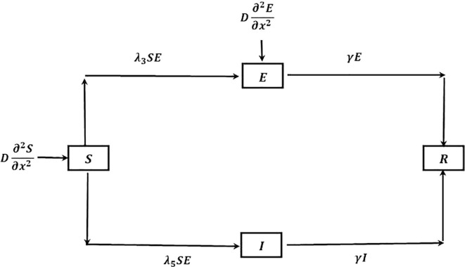
Due to proper quarantine of infective population and considering for citizens of several countries that needed to be quarantined for 14 days earlier to entering their topical countries or topical state, who comes outside their own country or own state respectively and treating them as infective, though the interaction between several classes of people, considered above, is reduced but not properly [18]. Because of daily life survival, some of the susceptible population comes in contact with some of the E class, like in market, medicine shop etc. In this model only the population of S and E classes are interact with each other, infected are to be separated in an isolated place. The corresponding model followed by the flow chart Fig. 2 is:

$$\frac{\partial S}{\partial t}=-{\lambda }_1\mathit{SE}+D\frac{{\partial }^{2}S}{\partial x^2},$$ (20)

$$\frac{\partial E}{\partial t}={\lambda }_3\mathit{SE}-\gamma E+D\frac{{\partial }^{2}E}{\partial x^2},$$ (21)

$$\frac{\partial I}{\partial t}={\lambda }_5\mathit{SE}-\gamma I\text{.}$$ (22)

$$\frac{\partial R}{\partial t}=\gamma (I+E)\text{.}$$ (23)

Fig. 2.

Flow of COVID-19 transmission for ‘proper quarantine case’.

It is easy to check that the system (20), (21) has infinitely many solutions. The following results show that the solutions of the system (20), (21) is non-negative and uniformly bounded.

Proposition 3

For a non-negative initial function, the system (20), (21) possesses a non-negative solution.

Proof

The proof is similar as Proposition (1. □

Proposition 4

For a non-negative non-trivial initial value let

$\left(S,E\right)\in {\left[C^{2,1}\left(\bar{\mathrm{\Omega }}\times [0,T_{\mathit{max}})\right)\cap C^{2,1}\left(\mathrm{\Omega }\times (0,T_{\mathit{max}})\right)\right]}^2$ be a solution of the system (20), (21) . Then $T_{\mathit{max}}=\infty$ and

$0<S(x,t)+E(x,t)⩽\mathit{max}\{{\left|\left|S_0\left(x\right)+E_0\left(x\right)\right|\right|}_{\infty }+{\left|\left|S_0^{\prime }\left(x\right)+E_0^{\prime }\left(x\right)\right|\right|}_{\infty }+{\left|\left|S_0^{″}\left(x\right)+E_0^{″}\left(x\right)\right|\right|}_{\infty },N\}$ , where prime denote the differentiation with respect to x.

Proof

The proof is similar as Proposition (2. □

$R_0$ for ‘proper quarantine case’: Due to ‘proper quarantine’ [6], the strict isolation [7] of infected individuals and considering for citizens of several countries that required to be quarantined for 14 days prior to entering their native countries or native state, who comes outside their own country or own state respectively, mainly the E class is dominated to spread the pandemic COVID-19. From the equation (21), the per capita increase of E class is given by

$$\frac{1}{E}\frac{\partial E}{\partial t}={\lambda }_{3}S-\gamma \text{.}$$

Which gives us the basic reproductive rate

$$R_0=\frac{{\lambda }_3{S}_0}{\gamma }\text{.}$$

If $R_0>1$, then every infected member of the population will emit the disease to leastwise one other member during the infectious epoch, and the model argue that the disease will propagate within the population. If not, then the disease is desired to fall through before overreaching a substantive fraction of total population. Therefore $R_0=1$ is a critical epidemiological grade. In other terms, pathogens with elevated equilibrium of contagion and subordinate rescue and mortality rates will gesture an ideal threat. The reciprocal of the removal rate is the average time interval during which an individual from both E and I class remain contagious, given by $\frac{1}{\gamma }$.

Re-parametrisation

For non-dimensionalisation, rescaling dependent variables $S,E,I,R$ by $S_0$, the initial susceptible population and independent variables as $x,t$ by $x_0$ and $t_0$ respectively, let $S=S_0{S}^{\ast },E=S_0{E}^{\ast },I=S_0{I}^{\ast },R=S_0{R}^{\ast },t=t_0{t}^{\ast },x=x_0{x}^{\ast }$, where $S_0,t_0$ and $x_0$ are the characteristic units used to scale the above variables. Putting these in the system (20), (23) we get

$$\frac{S_0}{t_0}\frac{\partial S^{\ast }}{\partial t^{\ast }}=-{\lambda }_1{S}_0{S}^{\ast }{S}_0{E}^{\ast }+D\frac{S_0}{x_0^2}\frac{{\partial }^2{S}^{\ast }}{\partial x^{*2}}$$

$$\frac{S_0}{t_0}\frac{\partial E^{\ast }}{\partial t^{\ast }}={\lambda }_3{S}_0{S}^{\ast }{S}_0{E}^{\ast }-\gamma S_0{E}^{\ast }+D\frac{S_0}{x_0^2}\frac{{\partial }^2{E}^{\ast }}{\partial x^{*2}}$$

$$\frac{S_0}{t_0}\frac{\partial I^{\ast }}{\partial t^{\ast }}={\lambda }_5{S}_0{S}^{\ast }{S}_0{E}^{\ast }-\gamma S_0{I}^{\ast }$$

$$\frac{S_0}{t_0}\frac{\partial R^{\ast }}{\partial t^{\ast }}=\gamma S_0(I^{\ast }+E^{\ast })$$

that is,

$$\frac{\partial S^{\ast }}{\partial t^{\ast }}=-{\lambda }_1{t}_0{S}^{\ast }{S}_0{E}^{\ast }+D\frac{t_0}{x_0^2}\frac{{\partial }^2{S}^{\ast }}{\partial x^{*2}}$$

$$\frac{\partial E^{\ast }}{\partial t^{\ast }}={\lambda }_3{t}_0{S}^{\ast }{S}_0{E}^{\ast }-\gamma t_0{E}^{\ast }+D\frac{t_0}{x_0^2}\frac{{\partial }^2{E}^{\ast }}{\partial x^{*2}}$$

$$\frac{\partial I^{\ast }}{\partial t^{\ast }}={\lambda }_5{t}_0{S}^{\ast }{S}_0{E}^{\ast }-\gamma t_0{I}^{\ast }$$

$$\frac{\partial R^{\ast }}{\partial t^{\ast }}=\gamma t_0(I^{\ast }+E^{\ast })$$

With $S^{\ast }(x,0)=1,E^{\ast }(x,0)=\frac{E_0}{S_0},I^{\ast }(x,0)=\frac{I_0}{S_0},R^{\ast }(x,0)=0$ as initial conditions; where $E_0$ and $I_0$ are respectively the initial population of E and I class.

Letting $\gamma t_0=1$ and $D\frac{t_0}{x_0^2}=1$, we get $t_0=\frac{1}{\gamma }$ and $x_0={\left(\frac{D}{\gamma }\right)}^{\frac{1}{2}}$. Thus we end up with the scaled model

$$\frac{\partial S^{\ast }}{\partial t^{\ast }}=-\mu S^{\ast }{E}^{\ast }+\frac{{\partial }^2{S}^{\ast }}{\partial x^{*2}},$$ (24)

$$\frac{\partial E^{\ast }}{\partial t^{\ast }}=R_0{S}^{\ast }{E}^{\ast }-E^{\ast }+\frac{{\partial }^2{E}^{\ast }}{\partial x^{*2}},$$ (25)

$$\frac{\partial I^{\ast }}{\partial t^{\ast }}=(\mu -R_0)S^{\ast }{E}^{\ast }-I^{\ast }\text{.}$$ (26)

$$\frac{\partial R^{\ast }}{\partial t^{\ast }}=I^{\ast }+E^{\ast }\text{.}$$ (27)

with $S^{\ast }(x,0)=1,E^{\ast }(x,0)=\frac{E_0}{S_0}$ , $I^{\ast }(x,0)=\frac{I_0}{S_0},R^{\ast }(x,0)=0$ and two dimensionless numbers $R_0$ and $\mu$ as $R_0=\frac{{\lambda }_3{S}_0}{\gamma }$ and $\mu =\frac{{\lambda }_1{S}_0}{\gamma }$ respectively.

The parameters ${\lambda }_1$, …, ${\lambda }_5,\gamma$ and D in the dimensional model have been reduced to only two dimensionless grouping $R_0$ and $\mu$.

Method of solution

In this model we investigate the local spread of an epidemic wave [13] of infection into a uniform susceptible population. We want to designate conditions for the existence of such travelling wave, its speed of propagation and, when it exists.

Looking for the one dimensional travelling wave solutions, let.

$S^{\ast }(x^{\ast },t^{\ast })=S^{\ast }\left(z\right),E^{\ast }(x^{\ast },t^{\ast })=E^{\ast }\left(z\right),I^{\ast }(x^{\ast },t^{\ast })=I^{\ast }\left(z\right),R^{\ast }(x^{\ast },t^{\ast })=R^{\ast }\left(z\right),z=x^{\ast }-{\mathit{ct}}^{\ast }$; where the wave speed c, have to be determine. The above consideration will gives us a travelling wave of constant shape in the direction of positive $x^{\ast }$-axis. Substituting the above consideration into the system (24), (27) we get the system of equations as

$$-c\frac{{\mathit{dS}}^{\ast }}{\mathit{dz}}=-\mu S^{\ast }{E}^{\ast },$$ (28)

$$-c\frac{{\mathit{dE}}^{\ast }}{\mathit{dz}}=R_0{S}^{\ast }{E}^{\ast }-E^{\ast },$$ (29)

$$-c\frac{{\mathit{dI}}^{\ast }}{\mathit{dz}}=(\mu -R_0)S^{\ast }{E}^{\ast }-I^{\ast },$$ (30)

$$-c\frac{{\mathit{dR}}^{\ast }}{\mathit{dz}}=I^{\ast }+E^{\ast }\text{.}$$ (31)

Proposition 5

For the positive constants $R_0,\mu ,c$ ; let the system (28), (29) possesses a solution $S^{\ast }\left(z\right)⩾0,E^{\ast }\left(z\right)⩾0$ with $S^{\ast }\left(0\right)=S_0^{\ast }=1$ , $E^{\ast }\left(0\right)=E_0^{\ast }>0$ . Then the long term behaviour of the system (28), (29) is characterized by $R_0$ , i.e., if $R_0<1$ , then $S^{\ast }\left(z\right)$ decreases to a limiting value $S^{\ast }\left(\infty \right)>0$ and $E^{\ast }\left(z\right)$ first increase and then decrease to 0. If $R_0>1$ , then $S^{\ast }\left(z\right)$ decreases to a limiting value $S^{\ast }\left(\infty \right)>0$ and $E^{\ast }\left(z\right)$ decrease to 0.

Proof

Addition of (28), (29) and integration over $(0,z)$ gives

$$0⩽S^{\ast }\left(z\right)+E^{\ast }\left(z\right)=\frac{\mu -R_0}{c}{\int }_0^z{S}^{\ast }\left(s\right)E^{\ast }\left(s\right)\mathit{ds}+\frac{1}{c}{\int }_0^z{E}^{\ast }\left(s\right)\mathit{ds}+1+E_0^{\ast }$$

The existence of unique non-negative solution on $[0,\infty )$ follows from the standard theory.

Since $\frac{{\mathit{dS}}^{\ast }}{\mathit{dz}}⩾0,S^{\ast }\left(z\right)$ converges to a limit $S^{\ast }\left(\infty \right)⩾0$. The boundedness of $\frac{{\mathit{dE}}^{\ast }}{\mathit{dz}}$ on $[0,\infty )$ follows from the boundedness of $S^{\ast }\left(z\right),E^{\ast }\left(z\right)$ on $[0,\infty )$ and

${\int }_0^{\infty }{E}^{\ast }\left(s\right)\mathit{ds}<\infty$,   ${\int }_0^z{S}^{\ast }\left(s\right)E^{\ast }\left(s\right)\mathit{ds}<\infty$. which implies that ${\lim }_{z\to \infty }{E}^{\ast }\left(z\right)=0$ and ${\lim }_{z\to \infty }{S}^{\ast }\left(z\right)E^{\ast }\left(z\right)=0$.

Division of equation (28) by $S^{\ast }\left(z\right)$ and integration over $(0,z)$ gives

$$S^{\ast }\left(z\right)=\mathit{exp}\left(\frac{\mu }{c}{\int }_0^z{E}^{\ast }\left(s\right)\mathit{ds}\right)$$

$\Rightarrow$   $S^{\ast }\left(\infty \right)=\mathit{exp}\left(\frac{\mu }{c}{\int }_0^{\infty }{E}^{\ast }\left(s\right)\mathit{ds}\right)\ne 0$ Now differentiating equation (29) with respected to z we get

$$\frac{d^2{E}^{\ast }}{{\mathit{dz}}^2}=-\frac{R_0}{c}\left[\frac{{\mathit{dS}}^{\ast }}{\mathit{dz}}{E}^{\ast }+S^{\ast }\frac{{\mathit{dE}}^{\ast }}{\mathit{dz}}\right]+\frac{1}{c}\frac{{\mathit{dE}}^{\ast }}{\mathit{dz}}$$

If there exists $z^{\ast }\in [0,\infty )$ such that ${\left(\frac{{\mathit{dE}}^{\ast }}{\mathit{dz}}\right)}_{z^{\ast }}=0$ then from the above equation we get

$${\left(\frac{d^2{E}^{\ast }}{{\mathit{dz}}^2}\right)}_{z^{\ast }}=-\frac{R_0}{c}{\left(\frac{{\mathit{dE}}^{\ast }}{\mathit{dz}}\right)}_{z^{\ast }}{\left(E^{\ast }\right)}_{z^{\ast }}<0$$

.

Thus if ${\left(\frac{{\mathit{dE}}^{\ast }}{\mathit{dz}}\right)}_{z^{\ast }}=0$ for some $z^{\ast }\in [0,\infty )$, then $E\left(z\right)$ is concave downwards.

Again from (29)

$$\frac{{\mathit{dE}}^{\ast }}{\mathit{dz}}=\frac{1}{c}\left(-R_0{S}^{\ast }\left(z\right)+1\right)E^{\ast }\left(z\right)$$

Then $E^{\ast }\left(z\right)$ increases at $z=0$ if $-R_0+1>0$, i.e. if $R_0<1$ and decreases at $z=0$ if $-R_0+1<0$, i.e. if $R_0>1$.

Therefore $E^{\ast }\left(z\right)$ has at most one peak. Also with the convergence of $E^{\ast }\left(z\right)$ to 0, our claim on $E^{\ast }\left(z\right)$ follows. Hence the proof.

Now the system (28), (31) can be represented as

$$S^{\ast ″}+{\mathit{cS}}^{\ast \prime }-\mu S^{\ast }{E}^{\ast }=0,$$ (32)

$$E^{\ast ″}+{\mathit{cE}}^{\ast \prime }+R_0{S}^{\ast }{E}^{\ast }-E^{\ast }=0,$$ (33)

$$I^{\ast ″}+{\mathit{cI}}^{\ast \prime }+(\mu -R_0)S^{\ast }{E}^{\ast }-I^{\ast }=0,$$ (34)

$${\mathit{cR}}^{\ast \prime }+(I^{\ast }+E^{\ast })=0\text{.}$$ (35)

where prime represents differentiation w.r.t. z. The above system consists of finding range of parameters considered above, for which there exists a solution with positive wave speed c and non-negative $S^{\ast },I^{\ast }$ such that

$E^{\ast }(-\infty )=E^{\ast }\left(\infty \right)=0,I^{\ast }(-\infty )=I^{\ast }\left(\infty \right)=0,0⩽S^{\ast }(-\infty )<S^{\ast }\left(\infty \right)=1$.

The conditions on $E^{\ast }$ and $I^{\ast }$ imply a pulse wave of infective population which propagates into the uninfected population. As time goes, the system (33), (34) changes by linearising, with $S^{\ast }\to 1,E^{\ast }\to 0$ and $I^{\ast }\to 0$ to get

$$E^{\ast ″}+{\mathit{cE}}^{\ast \prime }+(R_0-1)E^{\ast }\approx 0,$$ (36)

$$I^{\ast ″}+{\mathit{cI}}^{\ast \prime }-I^{\ast }\approx 0\text{.}$$ (37)

Phase plane analysis: From equations (36) a typical wave front solution is where $E^{\ast }$ at one side, say, as $z\to -\infty$, is at one steady state and as $z\to \infty$ it is at the other. So here we have to determine the value or values of c, for which the equation (36) has a non-negative solution $E^{\ast }$ which satisfies.

${\lim }_{z\to \infty }{E}^{\ast }\left(z\right)=0,{\lim }_{z\to -\infty }{E}^{\ast }\left(z\right)=1$.

In $(E^{\ast },U)$ phase plane.

$E^{\ast \prime }=U,U^{\prime }=-\mathit{cU}-(R_0-1)E^{\ast }$we have the phase plane trajectories as the solution of

$\frac{\mathit{dU}}{{\mathit{dE}}^{\ast }}=\frac{-\mathit{cU}-(R_0-1)E^{\ast }}{U}$which has one singular point for $(E^{\ast },U)$ as $(0,0)$. Corresponding to this singular point we define the matrix

$$A=\left(\begin{array}{cc}\hfill -c\hfill & \hfill -(R_0-1)\hfill \\ \hfill 1\hfill & \hfill 0\hfill \\ \hfill \hfill \end{array}\right)$$

whose eigenvalues are

$\frac{1}{2}\left[-c\pm \sqrt{c^2-4(R_0-1)}\right]$   $\Rightarrow$ $\left\{\begin{array}{cc}\hfill \mathit{stable}\mathit{node},\hfill & \hfill \mathit{if}{c}^2>4(R_0-1)\hfill \\ \hfill \mathit{stable}\mathit{spiral},\hfill & \hfill \mathit{if}{c}^2<4(R_0-1)\hfill \\ \hfill \hfill \end{array}\right)$ If $c⩾c_{\mathit{min}}=2\sqrt{R_0-1}$ then the singular point $(0,0)$ is a stable node. The case when $c=c_{\mathit{min}}$ gives us a degenerate node. If $c^2<4(R_0-1)$, it is a stable spiral; that is, in a neighbourhood of the origin, $E^{\ast }$ oscillates. By continuity disputes, in dimensional terms the range of c must satisfy

$$c⩾c_{\mathit{min}}=2\sqrt{R_0-1}=2\sqrt{\frac{{\lambda }_3{S}_0}{\gamma }-1},R_0>1\text{.}$$

No wave solution exists for $R_0<1$. So this condition is necessary for the spread of epidemic wave for $E^{\ast }$ class.

There are a typical travelling wave solution when $c⩽2\sqrt{R_0-1}$. As $E^{\ast }<0$ for some z, they are physically unrealistic, because in that case $E^{\ast }$ spirals around the origin. In this seance $E^{\ast }\to 0$ at the leading edge with decreasing oscillation around $E^{\ast }=0$.

From equations (37) a typical wave front solution is where $I^{\ast }$ at one side, say, as $z\to \infty$, is at one steady state and as $z\to -\infty$ it is at the other. In that case we have to determine the value or values of c for which the equation (37) has a non-negative solution $I^{\ast }$ which satisfies.

${\lim }_{z\to \infty }{I}^{\ast }\left(z\right)=0,{\lim }_{z\to -\infty }{I}^{\ast }\left(z\right)=1$.

In $(I^{\ast },V)$ phase plane.

$I^{\ast \prime }=V,V^{\prime }=-\mathit{cV}+I^{\ast }$we have the phase plane trajectories as solution of

$\frac{\mathit{dV}}{{\mathit{dI}}^{\ast }}=\frac{-\mathit{cV}+I^{\ast }}{V}$which has one singular point for $(I^{\ast },V)$ as $(0,0)$. Corresponding to this singular point we define the matrix

$$A=\left(\begin{array}{cc}\hfill -c\hfill & \hfill 1\hfill \\ \hfill 1\hfill & \hfill 0\hfill \\ \hfill \hfill \end{array}\right)$$

whose eigenvalues are

$\frac{1}{2}\left[-c\pm \sqrt{c^2+4}\right]$   $\Rightarrow$ $\mathit{saddle}\mathit{point}$. □

Analysis of analytical solution

Now solutions of the system (36), (37) are respectively given by

$$E^{\ast }\left(z\right)\propto \mathit{exp}\left[\frac{(-c\pm {\{c^2-4(R_0-1\left)\right\}}^{\frac{1}{2}})z}{2}\right]$$ (38)

and

$$I^{\ast }\left(z\right)\propto \mathit{exp}\left[\frac{(-c\pm {\{c^2+4\}}^{\frac{1}{2}})z}{2}\right]$$ (39)

As we required $E^{\ast }\left(z\right)\to 0$ and $I^{\ast }\left(z\right)\to 0$ with $E^{\ast }\left(z\right)>0$ and $I^{\ast }\left(z\right)>0$, these solutions can not oscillate about $E^{\ast }=0$ and $I^{\ast }=0$ respectively; otherwise $E^{\ast }\left(z\right)<0$ and $I^{\ast }\left(z\right)<0$ for some z. Then from the relations (38), (39), the wave speed c and $R_0$ must satisfy

$$c⩾c_{\mathit{min}}=2\sqrt{R_0-1}=2\sqrt{\frac{{\lambda }_3{S}_0}{\gamma }-1},R_0>1$$ (40)

and the threshold condition in dimensional terms is given by

$$R_0=\frac{{\lambda }_3{S}_0}{\gamma }>1$$ (41)

we expect such travelling waves derived from the fully non-linear system of equations will evolve into a travelling waveform with the minimum wave speed $c=2{(R_0-1)}^{\frac{1}{2}}$, except in exceptional conditions. The wave velocity for COVID-19, V say, in dimensional term is then given by

$$V={\left(\gamma D\right)}^{\frac{1}{2}}c=2{\left(\gamma D\right)}^{\frac{1}{2}}{[\frac{{\lambda }_3{S}_0}{\gamma }-1]}^{\frac{1}{2}}$$

The travelling wave solution for susceptible population $S^{\ast }$ cannot have a local maximum, since $S^{\ast \prime }=0$ there and the equation for $S^{\ast }$ shows that $S^{\ast ″}=\mu E^{\ast }{S}^{\ast }>0$, which indicate a local minimum. So $S^{\ast }\left(z\right)$ is a monotone increasing function of z. By linearising the equation (32) for $S^{\ast }$ as $z\to \infty$, where $S^{\ast }=1-s$, with s small, we get

$$s^{″}+{\mathit{cs}}^{\prime }-\mu E^{\ast }=0$$

with which $E^{\ast }\left(z\right)$ from (38),

$$S^{\ast }\left(z\right)~1-O\left(\mathit{exp}\right[\frac{(-c\pm {\{c^2-4(R_0-1\left)\right\}}^{\frac{1}{2}})z}{2}\left]\right)$$

and so, as $z\to \infty ,S^{\ast }\left(z\right)\to 1$ exponentially.

Results and discussion

In this paper for the epidemic COVID-19, we have investigated both analytical and numerical solutions for both the models ‘no quarantine case’ and ‘proper quarantine case’. From our analysis of analytical solution for both the models it is observed that for ‘no quarantine case’ as time goes, both the susceptible and latent infected population tend to zero and the total population will become infected where as for ‘proper quarantine case’ as time goes; the infected population decrease, latent infected population tend to zero and the total population will become susceptible.

For ‘no quarantine case’ we separately calculate the speed of spread of COVID-19 in both E and I class, which tells us that, as time goes, whether E or I class increase. After that we consider the Euclidean norm to calculate the wave velocity for the pandemic COVID-19 in total population, given by the relation (19). For ‘proper quarantine case’, due to proper quarantine for infected population, the speed of spread of COVID-19 only depend on E class. So the speed of spread of COVID-19 in E class is the wave velocity for the pandemic COVID-19 in total population, given by the relation (40).

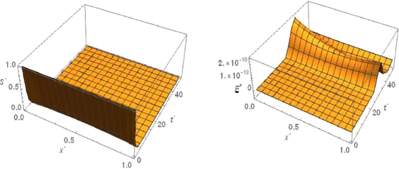
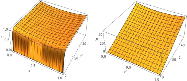
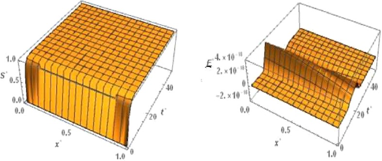
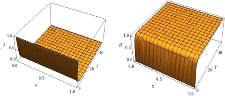
For ‘no quarantine case’ the numerical simulation of travelling wave solution of the system (6), (9) is done using Crank-Nicolson method. For the sake of convenience we truncate the time domain $[0,\infty )$ to $[0,50]$ and the one dimensional spatial domain $\mathrm{\Omega }$ to $[0,1]$. With respect to this boundary condition of $t^{\ast }$ and $x^{\ast }$, The boundary conditions of $S^{\ast }(x^{\ast },t^{\ast })),E^{\ast }(x^{\ast },t^{\ast })$ , $I^{\ast }(x^{\ast },t^{\ast })$ and $R^{\ast }(x^{\ast },t^{\ast })$ are considered as $S^{\ast }(x^{\ast },0)=S^{\ast }(x^{\ast },50)=1,S^{\ast }(0,t^{\ast })=S^{\ast }(1,t^{\ast })=0\text{;}{E}^{\ast }(x^{\ast },0)=E^{\ast }(x^{\ast },50)=E^{\ast }(0,t^{\ast })=E^{\ast }(1,t^{\ast })=0$ and $I^{\ast }(x^{\ast },0)=I^{\ast }(x^{\ast },50)⩾0,I^{\ast }(0,t^{\ast })=I^{\ast }(1,t^{\ast })=1$ and $R^{\ast }(x^{\ast },0)$=0 respectively. The 3D plots of $S^{\ast }(x^{\ast },t^{\ast }),E^{\ast }(x^{\ast },t^{\ast })$ $I^{\ast }(x^{\ast },t^{\ast })$ and $R^{\ast }(x^{\ast },t^{\ast })$ are shown in Figs. Fig. 3, Fig. 4 ,respectively with respect to $x^{\ast }$ and $t^{\ast }$ for the travelling wave solution. Based on above boundary conditions, numerical simulation shows that for the figure Fig. 3, the susceptible population $S^{\ast }(x^{\ast },t^{\ast })$ goes to zero in forward time and at any position $x^{\ast }$. From the figure Fig. 3 it is obvious that the latent infected population $E^{\ast }(x^{\ast },t^{\ast })$ first increase and after certain time it decrease and goes to zero in forward time at any position $x^{\ast }$. From the figure Fig. 4, it is observed that the infected population $I^{\ast }(x^{\ast },t^{\ast })$ increases and takes the value one in forward time at any position $x^{\ast }$. From the figure Fig. 4 we observe that the graph of removed population $R^{\ast }(x^{\ast },t^{\ast })$ is flat with respect to $t^{\ast }$, because there are no diffusion of $R^{\ast }$.

Fig. 3.

No quarantine case: Numerical simulation for Susceptible population $S^{\ast }(x^{\ast },t^{\ast })$ and Latent infected population $E^{\ast }(x^{\ast },t^{\ast })$ for the system of equations (6), (9) when $a=8\text{;}b=3\text{;}\mu =1.8,\left|\right|c|{|}_2=2.5$ and $R_0=2.5$.

Fig. 4.

No quarantine case: Numerical simulation for Infected population $I^{\ast }(x^{\ast },t^{\ast })$ and Removed population $R^{\ast }(x^{\ast },t^{\ast })$ for the system of equations (6), (9) when $a=8\text{;}b=3\text{;}\mu =1.8,\left|\right|c|{|}_2=2.5$ and $R_0=2.5$.

For ‘proper quarantine case’ the numerical simulation of travelling wave solution of the system (24), (27) is done. Like ‘no quarantine case’ here we also truncate the time domain $[0,\infty )$ to $[0,50]$ and the one dimensional spatial domain $\mathrm{\Omega }$ to $[0,1]$. With respect to this boundary condition of $t^{\ast }$ and $x^{\ast }$, the boundary condition of $S^{\ast }(x^{\ast },t^{\ast }),E^{\ast }(x^{\ast },t^{\ast }),I^{\ast }(x^{\ast },t^{\ast })$ and $R^{\ast }(x^{\ast },t^{\ast })$ are defined as by $S^{\ast }(x^{\ast },0)=S^{\ast }(x^{\ast },50)⩾0$, $S^{\ast }(0,t^{\ast })=S^{\ast }(1,t^{\ast })=1$, $E^{\ast }(x^{\ast },0)=E^{\ast }(x^{\ast },50)=E^{\ast }(0,t^{\ast })=E^{\ast }(1,t^{\ast })=0$ , $I^{\ast }(x^{\ast },0)=I^{\ast }(x^{\ast },50)=1,I^{\ast }(0,t^{\ast })=I^{\ast }(1,t^{\ast })=0$ and $R^{\ast }(x^{\ast },0)$=0. The 3D plots of $S^{\ast }(x^{\ast },t^{\ast }),E^{\ast }(x^{\ast },t^{\ast })$ $I^{\ast }(x^{\ast },t^{\ast })$ and $R^{\ast }(x^{\ast },t^{\ast })$ are shown in figures (5 and 6 , respectively with respect to $x^{\ast }$ and $t^{\ast }$ for the travelling wave solution. Based on above boundary conditions, numerical simulation shows that for the Fig. 5, the susceptible population $S^{\ast }(x^{\ast },t^{\ast })$ increases and goes to one in forward time and at any position $x^{\ast }$. From the figure Fig. 5 it is obvious that the latent infected population $E^{\ast }(x^{\ast },t^{\ast })$ first increase and after certain time it decrease and goes to zero in forward time at any position $x^{\ast }$. From the figure Fig. 6 we observe that the infected population $I^{\ast }(x^{\ast },t^{\ast })$ decrease and takes the value zero in forward time at any position $x^{\ast }$. From the figure Fig. 6 we observe that the graph of removed population $R^{\ast }(x^{\ast },t^{\ast })$ is increases in forward time and at any position $x^{\ast }$.

Fig. 5.

Proper quarantine case: Numerical simulation for Susceptible population $S^{\ast }(x^{\ast },t^{\ast })$ and Latent infected population $E^{\ast }(x^{\ast },t^{\ast })$ for the system of equations (24), (27) when c = 5, $\mathit{mu}=3$ and $R_0=2.5$.

Fig. 6.

Proper quarantine case: Numerical simulation for Infected population $I^{\ast }(x^{\ast },t^{\ast })$ and Removed population $R^{\ast }(x^{\ast },t^{\ast })$ for the system of equations (24), (29) when c = 5, $\mathit{mu}=3$ and $R_0=2.5$.

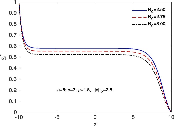
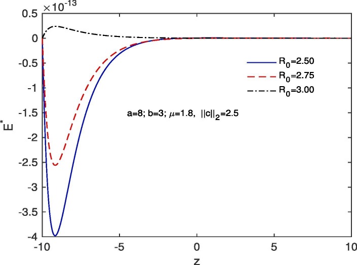
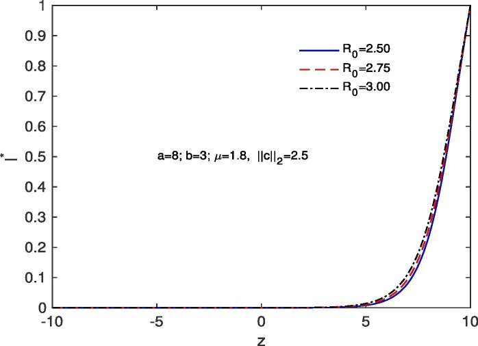
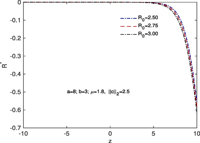
For ‘no quarantine case’, we solve the system (10), (13) numerically with boundary conditions $E^{\ast }(-\infty )=E^{\ast }\left(\infty \right)=0$, $S^{\ast }(-\infty )=1,S^{\ast }\left(\infty \right)=0,0⩽I^{\ast }(-\infty )<I^{\ast }\left(\infty \right)=1$. The estimation of parameters are given by $a=8,b=3,\mu =1.8,c=2.5$ and $2.5⩽R_0⩽3.00$. Based on those boundary conditions and the estimation of parameters, a numerical simulation is done for all of $S^{\ast },E^{\ast },I^{\ast }$ and $R^{\ast }$ populations with respect to z and the variations of Basic Reproduction number $R_0=2.50,R_0=2.75$ and $R_0=3.00$. In Fig. 7 we draw the graphs of $S^{\ast }$ with respect to z and the above stated variations of $R_0$. For all the variations of $R_0$ we observed that $S^{\ast }$tends to 0 as z approaches to $\infty$. As for an infectious disease (COVID-19 in our case) the basic reproductive number is the number of secondary infections delivered by a single infected individual in whole susceptible population and this quantity indicates the initial growth rate of the infected population and the potential for a large-scale epidemic, it is also noticed that for the larger value of $R_0$ the susceptible population will become more infected and the rate of convergence of the susceptible population $S^{\ast }$ to 0 becomes faster for a large population. In Fig. 8 we draw the graphs of $E^{\ast }$ with respect to z and for the variations of $R_0$. In this case for all the variations of $R_0$ we observed that the latent infected population $E^{\ast }$ tends to 0 as z approaches to $\infty$. In Fig. 9 we draw the graphs of $I^{\ast }$ with respect to z and the variations of $R_0$. For all the variations of $R_0$ we observed that $I^{\ast }$ tends to 1 as z approaches to $\infty$. It is also noticed that for the larger value of $R_0$ the volume of susceptible population $S^{\ast }$ decreases, whereas the volume of infected population $I^{\ast }$ increases. That is why the rate of convergence of the infected population $I^{\ast }$ to 1 becomes faster for the larger value of $R_0$ for a larger population. In Fig. 10 the graphs of $R^{\ast }$ with respect to z and for the variations of $R_0$ are drawn. For all the above stated variations of $R_0$ the removed population $R^{\ast }$ decreases as z approaches to $\infty$. This discussion guarantee us that for vno quarantine case’ the total population will become infected after certain time. That is why a ‘proper quarantine’ is essential, as a result we consider our next model as a ‘proper quarantine model’.

Fig. 7.

Variation of the susceptible population with z when $a=8\text{;}b=3\text{;}\mu =1.8,\left|\right|c|{|}_2=2.5$, with respect to the variation of $R_0$.

Fig. 8.

Variation of the latent infected population with z when $a=8,b=3,\mu =1.8,\left|\right|c|{|}_2=2.5$; with respect to the variation of $R_0$.

Fig. 9.

Variation of the Infected population with z when $a=8,b=3,\mu =1.8,\left|\right|c|{|}_2=2.5$; with respect to the variation of $R_0$.

Fig. 10.

Variation of the Removed population with z when $a=8,b=3,\mu =1.8,\left|\right|c|{|}_2=2.5$; with respect to the variation of $R_0$.

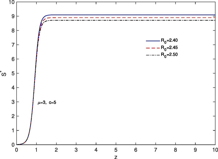
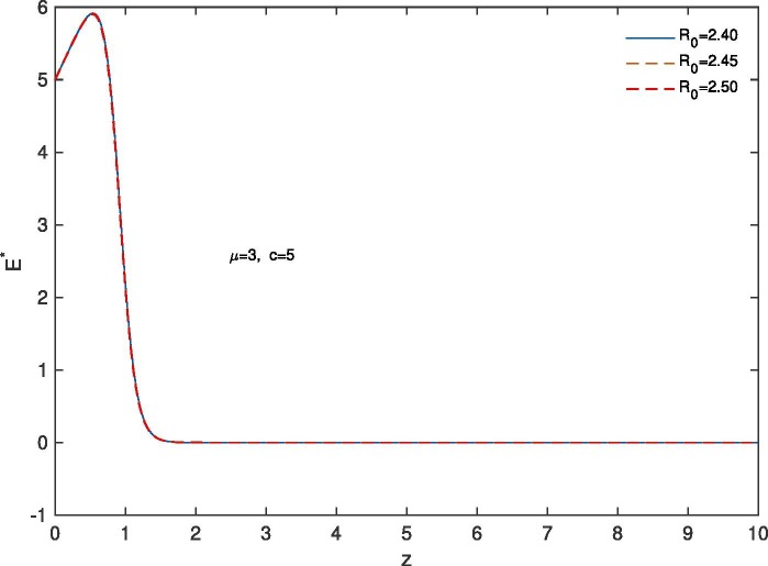
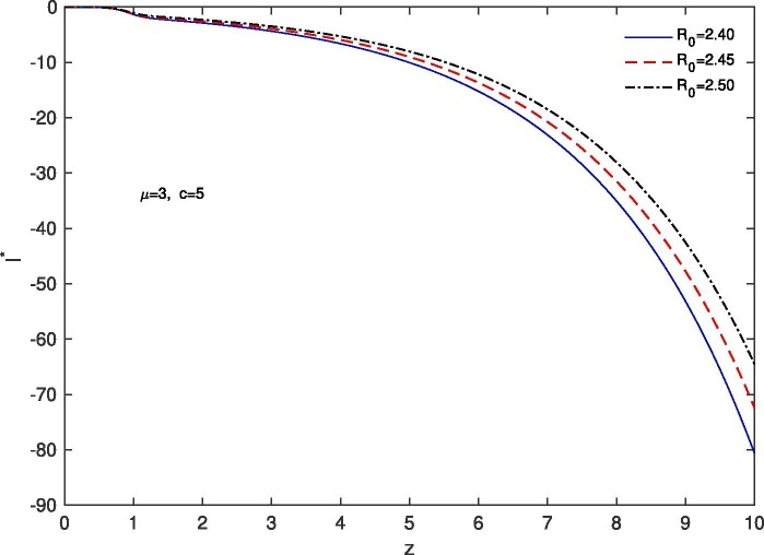
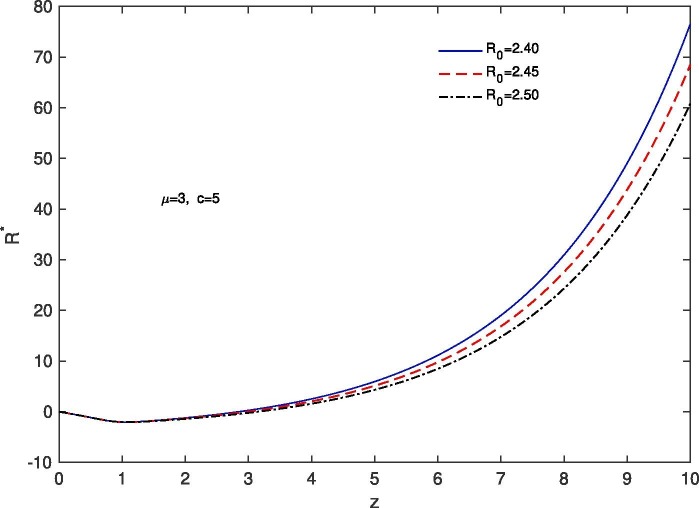
For ‘proper quarantine case’, we solve the system (28), (31) numerically with boundary conditions $E^{\ast }(-\infty )=E^{\ast }\left(\infty \right)=0$, $I^{\ast }(-\infty )=I^{\ast }\left(\infty \right)=0,0⩽S^{\ast }(-\infty )<S^{\ast }\left(\infty \right)=1$. The estimation of parameters are given by $\mu =3,c=5$ and $2.40⩽R_0⩽2.50$. Based on those boundary conditions and the estimation of parameters, a numerical simulation is done for all of $S^{\ast },E^{\ast }$, $I^{\ast }$ and $R^{\ast }$ populations with respect to z and the variations of the Basic Reproduction Number $R_0$ as $R_0=2.40$, $R_0=2.45$ and $R_0=2.50$.In Fig. 11 we draw the graphs of $S^{\ast }$ with respect to z and the variations of and $R_0$. For all the above stated variations of $R_0$ we observed that $S^{\ast }$ increases as z approaches to $\infty$. It is also noticed that for the larger value of $R_0$, the rate of increase of the susceptible population $S^{\ast }$ becomes slower. This happens because of ‘proper quarantine’ of infected individuals and proper isolation of latent infected population. In this case the number of secondary infection from a single primary infection is reduced and therefore the value of the Basic Reproduction Number $R_0$ is reduced. In Fig. 12 we draw the graphs of $E^{\ast }$ with respect to z and for the variations of $R_0$. In this case for all the variations of $R_0$ we observed that the latent infected population $E^{\ast }$ tends to 0 as z approaches to $\infty$. In Fig. 13 we draw the graphs of $I^{\ast }$ with respect to z and the variations of $R_0$. For all the variations of $R_0$ we observed that $I^{\ast }$ decreases monotonically as z approaches to $\infty$. It is also noticed that due to ‘proper quarantine’, for the smaller value of $R_0$, the rate of decrease of the infected population $I^{\ast }$ becomes faster. In Fig. 14 the graphs of $R^{\ast }$ with respect to z and for the variations of $R_0$ are drawn. For all the above stated variations of $R_0$ the removed population $R^{\ast }$ first decrease and after that it increases as z approaches to $\infty$. This discussion guarantee us that for ‘proper quarantine case’ the total population will become susceptible after certain time. Thus in the absence of vaccine, proper quarantine of infected individuals and proper isolation of latent infected individuals are very essential together with social distancing and use of mask.

Fig. 11.

Variation of the susceptible population with z when $c=5,\mu =3$; with respect to the variation of $R_0$.

Fig. 12.

Variation of the latent infected population with z when $c=5,\mu =3$; with respect to the variation of $R_0$.

Fig. 13.

Variation of the infected population with z when $c=5,\mu =3$; with respect to the variation of $R_0$.

Fig. 14.

Variation of the removed population with z when $c=5,\mu =3$; with respect to the variation of $R_0$.

An elementary public health intention is to fetch disease from over an epidemic threshold grade to under threshold grade, thereby excluding a threat of a large scale epidemic. That can accomplish through interventions that either directly impact the infectiousness of the pathogen, modify patterns of interaction so that the pathogen cannot easily spread within the population, or immunize partitions of the population. We call those three forms of intervention as contact reducing, transmission reducing, and immunizing [16].

There are some important enlightenment of the threshold result (41) like, the critical population density $S_c=\frac{\gamma }{{\lambda }_3}$ for the existence of epidemic wave for ‘proper quarantine case’; the critical transmission coefficient ${\lambda }_{3_c}=\frac{\gamma }{S_0}$ to the E class which, if not exceeded, obstruct the spread of the disease; the threshold mortality rate ${\gamma }_c={\lambda }_3{S}_0$ for E class which, if not exceeded, obstruct the spread of the disease etc. All of these have adhesion for control strategies [20], [26].If we can minimize the transmission measure ${\lambda }_3$ for COVID-19 to E class, it may be feasible to overstep condition (41) and therefore again obstruct the spread of the disease. This can be done by social distancing, proper quarantine of infective population and considering for citizens of several countries that needed to be quarantined for 14 days earlier to entering their topical countries or topical state, who comes outside their own country or own state respectively. Finally with $R_0>1$ as the threshold criterion we notice that an accidental inflow of the susceptible population can increase $S_0$ above $S_c$ and hence commence an epidemic.

All the mathematics for both models are done by the non-dimensionalisation, rescaling dependent variables $S,E,I,R$ by $S_0$, the initial susceptible population and independent variables $x,t$ by $x_0$ and $t_0$ respectively. Later on we found the value of $x_0$ and $t_0$. As the re-parametrisation for a mathematical model reduces number of parameters only, for the dimensional system in both our models we get the same result as re-parametrised system.

Conclusions

In the absence of vaccine for COVID-19, governments across the world are struggling to find ways to prevent the spread of COVID-19 and many countries are adoption lock down as a possible way to prevent the spread of the disease. But this strategy is not only hurting the economy of their respective countries, but also hurting the global economy.

In this article our investigation for the necessity of social distancing, isolation etc. for an infectious disease, proved that social distancing, proper quarantine of infective population and considering for citizens of several countries that required to be quarantined for 14 days prior to entering their native countries or native state, who comes outside their own country or own state respectively is one of the best possible way to stop the spread of COVID-19 with out lock down, in the absence of vaccine. This strategy can also save them from the destroy of their economy. Because, solving the model for ‘proper quarantine case’ by numerical method as well as analytical method we saw that the total population will become susceptible after certain time, where as for ‘no quarantine case’, we saw that the susceptible population become 0 after certain time. Not only for COVID-19, this model is also valid for any infectious disease, which transmit through contact.

We also make the following important observations. for both the model ‘no quarantine case’ and ‘proper quarantine case’, the system of diffusion equations possess non-negative solutions and the solution are uniformly bounded. For both models we derive the wave velocity for the epidemic, comparing them we get that the wave velocity for ‘no quarantine case’ is always greater than that of ‘proper quarantine case’.

Declaration of Competing Interest

The authors declare that they have no known competing financial interests or personal relationships that could have appeared to influence the work reported in this paper.

References

- 1.Allen L.J.S., Bolker B.M., Lou Y., Nevai A.L. Asymptotic profiles of the steady states for an SIS epidemic reaction-diffusion model. Discrete Continuous Dyn Syst. 2008;21:1–20. [Google Scholar]
- 2.Anderson RM, May RM. Infectious Diseases of Humans, Dynamics and Control, Oxford University Press: Oxford; 1991. Epidemiology and Infection. 108(1), 211–211.https://doi.org/10.1017/S0950268800059896.
- 3.Brandenburg A. Piecewise Quadratic growth during the 2019 novel corona virus epidemic, 2020. arXiv.https://doi.org/10.1016/j.idm.2020.08.014. Preprint at: http://arxiv.org/abs/2002.03638. [DOI] [PMC free article] [PubMed]
- 4.Bonabeau E., Toubiana L., Flahault A. The geographical spread of influenza. Proc R Soc Lond B. 1998;265:2421–2425. doi: 10.1098/rspb.1998.0593. [DOI] [PMC free article] [PubMed] [Google Scholar]
- 5.Capasso V. Global solution for a diffusive nonlinear deterministic epidemic model. SIAM J Appl Math 1978; 35: 274–284. ISSN: 00361399. url: http://www.jstor.org/stable/2100666.
- 6.CDC. Efficiency of quarantine during an epidemic of severe acute respiratory syndrome-Beijing, China, 2003; Morbidity and Mortality Weekly Report 52, no. 43, 1037–1040. [PubMed]
- 7.CDC. Informational bulletin, Public health guidance for community-level preparedness and response to severe acute respiratory syndrome (SARS) version 2, supplement D: Community containment measures, including non-hospital isolation and quarantine, 2004. URL: http://www.cdc.gov/ncidod/sars/guidance/D/pdf/lessons.pdf.
- 8.Evans L.C. 2nd ed. American Mathematical Society; 2010. Partial differential equations. [Google Scholar]
- 9.Feng W., Quan Y.H. Trend and forecasting of the COVID-19 outbreak in China. J Infect. 2020;80(4):469–496. doi: 10.1016/j.jinf.2020.02.014. [DOI] [PMC free article] [PubMed] [Google Scholar]
- 10.Ferguson N.M., Cummings D.A.T., Fraser C., Cajka J.C., Cooley P.C., Burke D.S. Strategies for mitigating an influenza pandemic. Nature. 2006;442(7101):448–452. doi: 10.1038/nature04795. [DOI] [PMC free article] [PubMed] [Google Scholar]
- 11.Ferguson NM, et al. Impact of non-pharmaceutical interventions (npis) to reduce covid-19 mortality and healthcare demand. London: Imperial College COVID- 19 Response Team, March 16 (2020).https://doi.org/10.25561/77482. [DOI] [PMC free article] [PubMed]
- 12.Hethcote H.W., van den Driessche P. Some epidemiological models with nonlinear incidence. J Math Biol. 1991;29:271–287. doi: 10.1007/BF00160539. CrossRef math-review Google Scholar. [DOI] [PubMed] [Google Scholar]
- 13.Kallen A., Arcuri P., Murray J.D.A. simple model for the spatial spread and control of rabies. J Theor Biol. 1985;116(3):377–393. doi: 10.1016/s0022-5193(85)80276-9. [DOI] [PubMed] [Google Scholar]
- 14.Li Q., Guan X., Wu P. Early transmission dynamics in Wuhan, China, of novel coronavirus-infected pneumonia. N Engl J Med. 2020 doi: 10.1056/NEJMoa2001316. [DOI] [PMC free article] [PubMed] [Google Scholar]
- 15.Murray JD. mathematical Biology, second edition. Berlin: springer-Verlag,1993; ISBN: 978-3-662-08542-4.
- 16.Pourbohloul B., Meyers L.A.V., Skowronski D.M., Krajden M., Patrick D.M., Brunham R.C. Modeling control strategies of respiratory pathogens. Emerg Infect Dis. 2005;11(8):1249–1256. doi: 10.3201/eid1108.040449. [DOI] [PMC free article] [PubMed] [Google Scholar]
- 17.Pinchover Y., Rubinson J. Cambridge University Press; New York: 2005. An introduction to partial differential equations. [Google Scholar]
- 18.Riou J., Althaus C.L. Pattern of early human-to-human transmission of Wuhan 2019 novel coronavirus (2019 nCoV), December 2019 to January 2020. Euro Surveill. 2020;25(4):2000058. doi: 10.2807/1560-7917.ES.2020.25.4.2000058. [DOI] [PMC free article] [PubMed] [Google Scholar]
- 19.Ruan S., Wang W. Dynamical behaviour of an epidemic model with a nonlinear incidence rate. J Differ Equ. 2003;188(1):135–163. doi: 10.1016/S0022-0396(02)00089-X. [DOI] [Google Scholar]
- 20.Tang B., Bragazzi N.L., Li Q., Tang S., Xiao Y., Wu J. An updated estimation of the risk of transmission of the novel coronavirus (2019-nCov) Infect Dis Model. 2020;5:248–255. doi: 10.1016/j.idm.2020.02.001. [DOI] [PMC free article] [PubMed] [Google Scholar]
- 21.Tian S, Hu N, Lou J, Chen K, Kang X, Xiang Z, Chen H, et al. Characteristic of COVID-19 infection in Beijing et al. J Infect 2020; 80(4):401–406.https://doi.org/10.1016/j.jinf.2020.02.018. [DOI] [PMC free article] [PubMed]
- 22.World Health Organization. Situation Report on Coronavirus Disease (COVID-19), 2020. https://who.int/emergencies/diseases/novel-coronavirus-2019/situation-reports.
- 23.You C, Deng Y, Hu W, Sun J, Lin Q, Zhou F, et al. Estimation of the Time-Varying Reproduction Number of COVID-19 Outbreak in China. SSRN, 2020; Preprint at: https://ssrn.com/abstract=3539694.https://doi.org/10.1101/2020.02.08.20021253. [DOI] [PMC free article] [PubMed]
- 24.Ying S, Li F, Geng X, Li Z, Du X, Chen H, et al.. Spread and control of COVID-19 in China and their associations with population movement, public health emergency measures, and medical resources. medRxiv, 2020; Preprint at:https://doi.org/10.1101/2020.02.24.20027623v1.
- 25.Zhang S., Diao M., Yu W., Pei L., Lin Z., Chen D. Estimation of the reproductive number of novel coronavirus (COVID-19) and the probable outbreak size on the Diamond Princess cruise ship: a data-driven analysis. Int J Infect Dis. 2020;93:201–204. doi: 10.1016/j.ijid.2020.02.033. [DOI] [PMC free article] [PubMed] [Google Scholar]
- 26.Zhong L., Mu L., Li J., Wang J., Yin Z., Liu D. Early Prediction of the 2019 Novel Coronavirus Outbreak in the Mainland China Based on Simple Mathematical Model. IEEE Access. 2020;8(51761–51769) doi: 10.1109/ACCESS.2979599. Published 2020 Mar 9. [DOI] [PMC free article] [PubMed] [Google Scholar]