

Abstract
Advances in protein tagging and mass spectrometry (MS) have enabled generation of large quantitative proteome and phosphoproteome data sets, for identifying differentially expressed targets in case-control studies. Power study of statistical tests is critical for designing strategies for effective target identification and control of experimental cost. Here, we develop a simulation framework to generate realistic phospho-peptide data with known changes between cases and controls. Using this framework, we quantify the performance of traditional t-tests, Bayesian tests, and the ranking-by-fold-change test. Bayesian tests, which share variance information among peptides, outperform the traditional t-tests. Although ranking-by-fold-change has similar power as the Bayesian tests, its type I error rate cannot be properly controlled without proper permutation analysis; therefore, simply relying on the ranking likely brings false positives. Two-sample Bayesian tests considering dependencies between intensity and variance are superior for data sets with complex variance. While increasing the sample size enhances the statistical tests’ performance, balanced controls and cases are recommended over a one-side weighted group. Further, higher peptide standard deviations require higher fold changes to achieve the same statistical power. Together, these results highlight the importance of model-informed experimental design and principled statistical analyses when working with large-scale proteomic and phosphoproteomic data.
Keywords: quantitative phosphorpoteomics, Bayesian statistics, empirical variance, proteomics, multiplex, two-sample, bioinformatics, neuroproteomics, hierachical simulation, sample size
Introduction
Cellular responses depend on the absolute level of proteins present in the cell, and also the relative activity of those proteins, which are regulated by a host of post-translational modifications. Phosphorylation is arguably the most common, and surely most extensively studied post-translational modification, central for regulating diverse functions of proteins, including enzymatic activity, protein localization, protein-protein interaction, ion channel activation and inactivation, etc.
Mass-spectrometry based proteomics is a powerful tool to quantify phosphorylation levels in complex cellular systems. In particular, isotope labelling technologies such as iTRAQ1 and TMT2 have allowed relative quantification of proteins and phosphorylation levels in multiple samples in a single experimental run, to identify differentially regulated protein or phosphorylation sites in case-control studies. Technical and instrumentation advancement now enable the quantification of more than 100,000 peptides, 10,000 proteins, and 10,000 unique phosphorylation sites in each run.3–5 This approach promises to capture global phosphorylation changes at the proteome level.
Despite technological advances in mass-spectrometry protocols and computational power, identification of significant targets are hindered. Within general modern mass spectrometry pipelines, the measured intensity of each peptide is reported as either the height of or the area under the peak corresponding to the given peptide.4 Given this intensity data, differential expression will be determined by testing whether the mean intensities of the peptide measured in channels corresponding to each condition significantly differs, in the background of tens or hundreds of thousands peptides. Generally speaking, the effective sample size for each phosphorylation site is very low, often just one peptide with less than 5 replicates per condition. Given 1) the high variance in the data due to inherent biological and technical variability, and 2) the relatively small sample size due to technical limits for isobaric tags, cost, and sample availability, it remains challenging to positively identify significant targets from proteomic and phosphoproteomic data sets. In some cases, target identification was achieved by the fold-change test followed by validations using other approaches, e.g.6,7 The significance of differential expression can be achieved with a two-sample t-test for independent samples or a one-sample t-test for paired samples for each peptide or phospho-peptide, e.g.8 However, the power and specificity of the tests are weakened by the small sample size. In practice, when working with such large data sets, the overall variance among peptides within all samples needs to be taken into consideration to better estimate the variance of any single peptide. A very similar challenge has been encountered in the analysis of gene expression data from microarray experiments, promoting the development of statistical tools addresses these concerns. Two of the most successful tools of empirical Bayesian tests, the moderated t-test (ModT) implemented in the limma R package,9 and the regularized t-test (RegT) available on the Cyber-T web server,10 rely on a Bayesian treatment to share variance information between peptides and increase the effective sample size. In contrast to non-parametric tests such as the Wilcoxon rank-sum test11 or Bayesian mixture models,12 these tests provide a principled estimator of the standard error of the fold change estimator. Such methods have become de-facto standards in microarray settings.13 However, the feasibility and robustness of these statistical tools in analyzing quantitative proteomic data, as well as the comparison among them, has not been fully explored.
We aim to evaluate the performance of empirical Bayesian tests, namely ModT and RegT, in comparison to the ranking-by-fold-change test and traditional t-tests using simulated data on the phospho-peptide level. In addition, we investigate how the data variance and the design of the proteomic experiment will affect the performance of the statistical tests.‘
Methods
Simulations
Our simulation framework is designed to produce a realistic distribution of log2 fold changes and intensities, with variability similar to empirical mass spec results. Similar to other studies,14–16 we log-transform the data for variance stabilization, and assume that the distribution of the log2 intensity of each peptide or protein is approximately normal. Our sampling framework is described by the following equations, which construct a hierarchical model to mimic the realistic data properties. Here, we adopt the convention that bold symbols are random variables, while non-bold variables are constant.
| (1) |
| (2) |
One of the following three assumptions on the variances were used in the hierarchical model:
| (3) |
| (4) |
| (5) |
Each measurement xij corresponds to the intensity of peptide i as measured in channel j, in either control (xc) or case (xe) conditions.
| (6) |
| (7) |
We first sample the “true” log2 mean abundance μi of each peptide i from a normal distribution described by the fixed parameters μ0 and σ0, reflecting inter-peptide biological variability and subsequently sample the intensity of each channel or sample xij around μi, reflecting biological and technical variability between samples. The spread of xij around μi is controlled by a peptide variance σ2 and a normal distribution. Our default simulation parameters are taken from an empirical data set.17 σ2 can be a fixed parameter or randomly sampled from an inverse gamma distribution, which captures the empirical distribution of sample peptide variances in real-world mass spectrometry data. Examples of the sampled distribution of intensities and variances are presented in Figure 1A for a fixed variance and in Figure 1B, a randomly sampled variance. In real proteomics data sets, the variance is high for low measured peptide intensities due to technical limitations. Randomly sampled biological variance can be scaled using the normalized average peptide variance for small intervals of empirical peptide intensities to incorporate this technical variance (Figure 1C). Variance dependence in empirical data is displayed in Figure 1D. See Figure 1E for the visualization of the model.
Figure 1: Overview of the simulation framework.

A-D) Scatterplots of the sample variance versus the sample mean log intensity for each peptide under the uniform (A), inverse gamma (B) or inverse gamma with a mean-variance trend (C) variance models, and for empirical data (D). The simulation models and experimental flow are shown on the top panels.
E) Bayesian network in plate notation describing the statistical model for the data simulation process. Fixed parameters are indicated in grey circles with their default values, random variables in white circles, and rectangles indicate repeated groups of variables. Each random variable is annotated with the distribution conditioned on the parent variables.
Statistical Tests
The ranking-by-fold-change Test (FC)
The ranking-by-fold-change test ranks peptides by the absolute value in the difference of the log2 peptide intensities in the case and control conditions.
| (8) |
where and denote the mean log2 peptide intensities of the case and the control channels, respectively. An arbitrary threshold is used to identify significant targets.
One-sample t-test
The one-sample t-test is applicable only for experiments with balanced numbers of case and control channels, and the experiments of case and control are paired. Hence, the difference between the log2 intensities for each paired case-control channels is taken as an independent measurement of the log2 fold change between the case and control peptide quantity. The test statistic
| (9) |
is t-distributed with n − 1 degrees of freedom under the null that the mean intensities in the two channels are equal, where denotes the mean log2 fold change between the case and control peptide quantity and n is the number of paired channels.
Two-sample t-test
The two-sample t-test treats each log2 channel intensity as a separate measurement of the true peptide abundance, and tests whether the mean control and case intensities are equal. Under the assumption that the log2 intensities of the control and experimental conditions are normally distributed and have equal variances, the test statistic
| (10) |
is t-distributed, with ne + nc − 2 degrees of freedom under the null that the mean intensities in the two channels are equal, where ne and nc denote the number of case and control channels respectively and and are the case and control sample variances defined analogous to above.
Regularized t-test (RegT)
The regularized t-test, introduced by10 on the Cyber-T web server, regularizes the ordinary t-statistic using variance information pooled across samples with similar intensities. The distribution of log2 intensities is assumed to be normal, and combined with a Bayesian conjugate prior over the variance of each peptide the test statistic takes the form
| (11) |
and are the mean of the posterior estimator of the peptide variance given the observed intensities, defined by
| (12) |
for each case respectively, where s2 is the respective sample variance. ν0 reflects the degree of belief in the prior, and controls the strength of regularization. For any given peptide, the prior variance is the running average of the variances of peptides over a window of size w, where peptides are ranked by average intensity. The probability of this statistic under the null hypothesis is described by a t-distribution with n − 2 + ν0 degrees of freedom. For our analysis, the default parameter settings of ν0 = 10 and w = 101 were retained.
Moderated t-test (ModT)
The moderated t-test,18 as implemented in the limma R package,9 evaluates any number of contrasts between the coefficients of a linear model. For our purposes, it suffices to analyze the one-sample and two-sample case-control comparison cases.
For a one-sample test, the data y is the difference between the log2 intensities for each paired case-control channel. In the two-sample case, the data y contains all control and case channels.
The coefficients β of the following linear model are estimated using the least squares estimator .
| (13) |
Under the null hypothesis, the difference between the control and case channels, β (1-sample) and β2 (2-sample), is expected to be 0. Similar to the RegT, the variance is regularized according to a Bayesian conjugate prior to yield a t-statistic estimator
| (14) |
where
| (15) |
and the variance estimate before moderation is the residual sample variance as used in the t-tests above. In this case, instead of a priori selecting the background degrees of freedom d0 and pooling the peptide variances to estimate , ModT fits a scaled F-distribution to the distribution of peptide sample variances and derives estimates of and d0 from this fitted distribution.
Limma offers a robust version of ModT19 that reduces the effect of high variance outliers (ModT-robust) and a mean-variance trend option (ModT-trend) that lets the prior variance depend on the log-intensity of each peptide.
The sensitivity and accuracy of each method in each simulation is quantified using the receiver operating characteristic (ROC) curve. This curve plots the true positive rate (TPR) against the false positive rate (FPR) as the p-value cutoff for significance varies. An example ROC curve from one simulation run is shown in Figure S1A. The area under the ROC curve (AUROC) serves as a scalar summary statistic which compares the relative performance of two or more classifiers. Formally, the AUROC measures the probability that a randomly chosen positive example ranks above a randomly chosen negative example; in practice, it can be loosely interpreted as the expected accuracy of the metric in ranking changed peptides above unchanged ones. In addition, we calculate the partial AUROC (pAUROC), which describes the area under the ROC curve in the region of low FPR (calculated from partial ROC, Figure S1B). pAUROC is a preferred measure in biological classification, as classifiers with high sensitivity are of limited utility when the FPR is high.20 For our analysis, we set a fixed threshold at the true FPR ≤ 0.05 for all tests. This normalizes the comparison, but has the disadvantage of ignoring the actual p-values of the data points. To address this issue, we separately evaluate the distribution of p-values and the performance around the 0.05 threshold of selected methods. For statistical completeness, we also calculate the area under the precision-recall curve (AUPRC, calculated from PRC, Figure S1C), which can be preferable for skewed data with a preponderance of negative examples.21,22
This sampling framework allows us to vary selected parameters in our simulations, including 1) the number of peptides (Figure S2); 2) the percentage of significantly perturbed peptides (Figure S2), 3) the fold change of the perturbed peptides (Figure 3); 4) the relative variance of the peptide means and measurements (Figures 3 and 4); and 5) the number of channels (Figure 5).
Figure 3: Performance of statistical tests with different variance models and a range of fold changes.

A,C,E) Simulation models using the uniform variance model (A), inverse gamma variance (C) or inverse gamma variance with a mean-variance trend (E). All parameters are fixed at the default value except for the fold change perturbation (FC, highlighted in crimson) applied to changed peptides.
B,D,F) pAUROC performance for each method quantified over 500 rounds of simulation under the uniform (B), inverse gamma (D) or intensity dependent inverse gamma variance (F) variance models across a range of fold change “spike-ins”.
Figure 4: TPR and FDR considerations of statistical tests with different variance models.

A) Simulation model using uniform variance, for data analyzed in B, S4A and S4B.
B) Mean FDR and TPR performance for selected methods over 500 rounds of simulation as fold change varies using either nominal (lighter lines) or BH adjusted (thicker lines) p-values at significance threshold of p < 0.05.
C) Simulation model using inverse gamma variance, for data analyzed in D, S4C and S4D.
D) Mean FDR and TPR performance for selected methods, similar to B.
E) Simulation model using inverse gamma variance with a mean-variance trend, for data analyzed in F, S4E and S4F.
F) mean FDR and TPR performance for selected methods, similar to B.
Figure 5: Performance of statistical tests with different sample sizes.

A-B) Simulation model using inverse gamma variance with a mean-variance trend (A) and pAUROC performance (B) quantified over 500 rounds of simulation. All parameters are fixed at the default value except for the number of case and control channels.
C-D) Simulation model using inverse gamma variance with a mean-variance trend (C) and pAUROC performance (D) quantified over 500 rounds of simulation. The total number of channels is fixed at 10, and the relative number of case and control channels is varied.
The seed empirical data for simulation is provided in the supplemental information. The code and the simulated data is in a public GitHub repository with a description of how to use the functions: https://github.com/hmsch/proteomics-simulations
Results and Discussion
Control of the type I error rate.
We first evaluated the distribution of p-values generated by each statistical test on a null simulation, where all peptides had no significant fold change (Figures 2A, 2C, 2E). Under these conditions, we expect the distribution of p-values to be uniform between 0 and 1. A different distribution of p-values obtained from the tests would indicate a failure to properly control the false positive rate. Among 9 tested methods, 7 produced approximately uniform p-value distributions, showing that they properly control the type I error rate, with the notable exception of the moderated t-tests when using the ‘robust’ regression option (Figures 2B, 2D, 2F). Given the distorted p-value distribution, we discarded the robust regression moderated t-test from the remainder of the analysis. Additionally, the one-sample ModT-trend test incorporating a mean-variance trend deviates from a uniform distribution for very small p-values when using a simulation with randomly sampled variances from an inverse gamma distribution (Figures 2D, 2F).
Figure 2: Control of the type I error rate by different statistical tests.
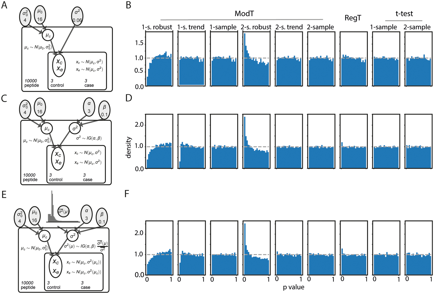
A,C,E) Simulation models for null data generation under the uniform (A), inverse gamma (C) or inverse gamma with a mean-variance trend (D) variance models. The control and experimental intensities are drawn from the same distribution with no perturbation.
B,D,F) p-value distributions for each method plotted with null data. The expected uniform distribution of p-values is indicated on each plot with the dotted line. All methods except the “robust” ModT produced an approximately uniform distribution.
It is important to note, that in this simulated null data, we still detected certain peptides with large fold changes between control and experimental conditions, which would be counted as significant events using the ranking-by-fold-change method. Anything detected using the fold change threshold method is a false positive under these conditions. There is no plausible control of the type I error rate using just a threshold for the fold change. In this case, the permutation analysis can be used to exact type I error rate.23,24 However, the effectiveness of the permutation analysis is dependent on the sample size to generate enough distinct numbers of shuffle to simulate null hypothesis.23 Therefore, the ranking-by-fold-change test is not recommended as a single statistical test for significance.
Bayesian statistics and the ranking-by-fold-change test perform superior to t-tests.
We started the first series of simulations by approximating a classic “spike-in” experiment (simulation model see Figure S2A). A set of distinct peptides with a predetermined nonzero fold change was added to samples containing an unperturbed background mixture of peptides. The base simulation generated 10,000 independent peptides, of which 9,000 were “background” with a true fold change of 0, and 1,000 (10%) were “spike-in” with a fixed nonzero fold change. Changing the sample size (1,000 and 100,000 peptides) and proportion of perturbed peptides (4% and 25%) had minimal effect on the performance of the statistical tests, as measured by the pAUROC (Figure S2B).
A range of nonzero fold changes were implemented in the simulation to visualize how the accuracy of each test evolves as the true fold change increases. The data were simulated using either a constant background variance (Figure 3A) across all peptides, randomly sampled variance for each peptide from an inverse gamma distribution (Figure 3C) or randomly sampled variance scaled according to the mean-variance dependency in empirical data (Figure 3E). AUROC, pAUROC and AUPRC statistics were calculated for each fold change across 500 rounds of simulation (pAUROC, shown in Figures 3B, 3D and 3F, AUROC and AUPRC in Figure S3A–F). As the pAUROC distribution (Figure 3B) shows, the power of these tests depends upon the size of the fold change. All methods perform badly when the fold change is small compared to the variance. As the fold change increases, the performance of all methods increases. Notably, in the intermediate region, where the log2 fold change lies between 0.3 and 1.0, distinctions between the methods are evident. The Bayesian statistics dramatically outperform the naive t-statistics for all three variance models. Surprisingly, simply ranking peptides by the absolute fold change difference between the case and control samples yields performance approaching the empirical Bayesian tests. Under the lower-complexity uniform variance simulation model, fold change ranking slightly outperforms RegT and equals ModT (Figure 3B). If more complex variance between peptides is assumed, as with the inverse gamma distributed variances, the empirical Bayesian tests slightly outperform the fold change ranking and are superior to traditional t-tests (Figure 3D). In this case both RegT and ModT (2-sample) perform equally well. The moderated 1-sample t-test taking into account a mean-variance trend over performs in this case although there is no mean-variance trend in the simulated data (Figure 1C). As evident in Figures 2D and 2F this test struggles to control the type I error. If a mean-variance dependency is assumed, as with the inverse gamma distributed variance scaled depending on peptide intensities, Bayesian tests that assume a dependency between intensity and variance outperform the other methods including ranking by fold change (Figure 3F).
In light of the good performance of the fold change ranking (Figure 3B and 3D) and the lack of type I error control, we conclude that it is acceptable to prioritize or rank hits based on the fold change when the existence of significant changes can be otherwise established. However, because it is impossible to set a principled threshold using fold change alone, this metric should not be applied to determine the presence of significant changes. Because the ranking-by-fold-change test performs well as a prioritization scheme, we retained it during the remainder of the analysis.
Two-sample Bayesian tests are superior for identifying significant targets in data sets with more complex variance.
In practice, significant targets from the phopsphoproteomics were identified using a cut-off from either nominal p-value or Benjamini-Hochberg (BH) adjusted p-value, calculated from selected statistical tests.25 To evaluate how the empirical Bayesian tests and t-tests report the statistical significance, we visualized the relationship between fold changes and either nominal or adjusted p-values using volcano plots and counts of postive and negative hits (example with FC = 0.5, shown in Figure S4) from simulated data (Figure 4A, 4C and 4E), and calculated TPR and FPR as illustrated in Figure 4B, 4D and 4E.
Under the low-complexity uniform variance model, all statistical tests captured nominally significant targets (FC = 0.5, shown in Figure S4, top panels). With ModT, the nominal p-values were strongly correlated with the mean fold change, because under conditions where the variance estimate is consistent across all peptides, ModT shrinks the individual sample variances more strongly compared to RegT, which uses a fixed number of pseudo-observations for normalization. Because the traditional t-tests do not share variance information, the relationship between p-values and fold changes was not strongly correlated. Using adjusted p < 0.05 as a cut off, we can calculate the percentage of true positives and false positives for each method from the simulations (FC = 0.5, shown in Figure S4B, 4B, S4D, 4D and S4F, 4F). As expected (Figure 2B), the FPRs were similar among all five tests. However, the empirical Bayesian tests had a higher TPR. The traditional t-tests have a higher FDR, decreasing the confidence for target identification. When the p-values are BH adjusted, traditional t-tests failed to report significant targets using p < 0.05 as a cut off, whereas empirical Bayesian tests reported significant targets (FC = 0.5, shown in Figure 4B, bottom panel). Although with adjusted p-values, empirical Bayesian tests showed lower FPR, resulting in low FDR, the analyses suffer from high FNR with the small fold change (FC = 0.5, shown in Figure 4C). Figure 4D shows the evolution of the TPRs and FDRs derived from the nominal and adjusted p-values, as the fold change increases. As expected, with a larger fold change, the TPR increased, and the FDR derived from nominal p-value decreased. The analysis shows that FDR was high with nominal p-values. Adjusting p-values successfully controlled the FDR to below 0.05, as expected. The lower FDR after adjustment provides greater certainty that significant peptides represent true biological changes. However, one should note that the TPR also decreased after adjustment; therefore, it is prudent to reemphasize that a non-significant p-value reflects only a failure to reject the null hypothesis and should not be interpreted as conclusive evidence against a true change. After adjustment, ModT outperforms RegT over the region in which the TPR progression is the most pronounced.
Under the high-complexity inverse gamma variance model, many attributes of the nominal p-value distribution are similar to that under the uniform variance model. First, all statistical tests captured nominally significant targets (FC = 0.5 shown in Figure S4C, top panel). Second, the empirical Bayesian tests gave better correlation between nominal p-values and the mean fold change (FC = 0.5 shown in Figure 4F). Third, the empirical Bayesian tests had a higher TPR, and the traditional t-tests had a higher FDR (FC = 0.5, shown in Figure S4D). However, ModT displayed much less shrinkage of the sample peptide variances towards a common mean, as evidenced by the reduced correlation between nominal p-values and the mean fold change (Figure S4C, top panel). When the p-values are BH adjusted, the moderated t-tests reported very few significant targets (Figure S4D), even though the ranking was maintained in the data distribution, due to this reduced shrinkage. This reflects a feature of the ModT implementation: if the estimated pooled variance differs greatly between peptides, the strength of the variance regularization is reduced. In contrast, RegT uses a fixed regularization independent of the empirically pooled variance, and more strongly pools the sample variances (Figure S4D). When we quantified the performance of these methods over a range of fold changes, the relative performances of ModT and RegT switched places. RegT quite dramatically outperforms ModT, with a greater TPR over the entire fold change range. However, at lower fold changes where the TPR is low, the FDR for RegT is not properly controlled even after adjustment (Figure 4D). Together, this implies that small sets of significant hits in the low fold change region produced by RegT are likely to contain a significant proportion of false positives. Given the extremely low TPR at lower fold changes, one should expect no significant discovery in this range using any methods.
For simulated data with a mean-variance dependency (Figure 4E), all Bayesian tests display fewer shrinkage of the sample peptide variances towards a common mean or trend than for the simpler variance models, as evidenced by the reduced correlation between nominal p-values and the mean fold change (Figure S4E, top panel). For this complex variance model, ModT incorporating a mean-variance trend has a higher TPR than ModT without this feature as expected (Figure 4F). While its TPR is lower than for RegT, its FDR does not suffer for lower fold-changes. Hence, targets identified using the 2-sample ModT with the variance trend option are more likely to be true positives than for RegT (Figure S4F).
Balanced sample sizes yield optimal performance.
Current labeling technologies allow for between 4 and 10 channels in a single run. With the limited channel numbers in proteomics and phosphoproteomics, there is the tradeoff between the number of the total case channels, and the number of control channels to capture the control variance. The statistical benefit is not intuitively accessible.
We first examined how the sample size affects the performance of each test under the model shown in Figure 5A (associated AUROC shown in Figure S5). The log2 fold change was fixed at 0.5, and the inverse gamma variance model with a mean-variance dependence was used. As expected, increasing the number of replicates/channels increases the accuracy of all tests (Figure 5B). However, the effect is not uniform. With lower channel numbers (2 controls vs 2 cases, or 3 controls vs 3 cases), ModT two-sample t-test performed better compared to RegT and fold change. RegT improved its performance over both fold change and ModT as the number of channels increased. As expected, the power of the analysis benefits from increasing sample sizes to allow maximal statistical power.
We next investigated the effect of imbalanced number of case and control channels on the performance of the statistical tests (Figure 5C). Given a total of 10 channels, we tested different combinations of case and controls channel numbers (1 vs 9, 2 vs 8, 3 vs 7, 4 vs 6, 5 vs 5). One-sample ModT was only tested with the 1 vs 9 condition, in which the nine case channels were ratioed to the one control channel; and with the 5 vs 5 condition, in which channels were arbitrarily assigned in pairs. All statistical tests gave the worst performance in the 1 vs 9 condition. The performance improved when channel assignment geared toward more balanced combinations. In fact, the 2 vs 8 condition already greatly improved the performance of the statistical tests, and the performance was the best in the 5 vs 5 condition. Our results indicate that taking into consideration the variance in both the control and the case groups is critical for optimal performance in a fixed number of channels, and balanced sample size for cases and controls is the best experimental practice for this purpose.
In many quantitative proteomics experimental design, a reference channel is used to normalize across multiple TMT-plex runs and increase the sample size when the sample processing and sample size are not the rate limiting factor. Depending on how the channels are arranged, the test statistical frameworks may or may not directly work. If we follow the similar setting describe in the paper, i.e., half channels are for “case” group and half for the “control” group, while each TMT-plex run spares one channel as a reference channel (for normalizing cross multiple TMT-plex runs), then our statistical framework should in principle apply. This is because our concerned response variable is the relative change (i.e., log fold change, or the log ratio between the intensities of the case and the control). In the case of the pair-wised t-test, the intensity of the reference will be cancelled out. As for other two-sample t-tests and the data generation process, it could be reasonable to assume that the reference channel perfectly rescales the log ratios cross different runs into the same normal distribution. Meanwhile, we could also assume that different TMT-plex runs end up with extra variations. Then an extra run/batch effect should be modeled (for example, in equation (3) we could replace to be to be dependent on the run r). In this case, further study would be needed to address the influence of the extra variation.
Higher peptide variance requires higher fold changes to achieve the same statistical power.
The peptide variance influences the performance of the statistical tests. When fixing the pAUROC score at approximately 0.75, there is a linear relationship between the peptide standard deviation and the smallest fold change necessary to achieve this score for Bayesian tests as well as a standard two-sample t-test (Figure 6). Bayesian tests reach pAUROC = 0.75 at drastically lower fold changes than the naive two-sample t-test. Together with the results from Figures 3 and 4, this highlights the importance of moderating or regularizing the peptide variance using global estimates to achieve maximum statistical power at low fold changes and high variance.
Figure 6: Performance of statistical tests with different peptide standard deviations.

A) Simulation model using inverse gamma variance with a mean-variance trend. Different fold changes and peptide variances were used (B).
B) Estimated fold changes necessary for pAUROC=0.75 given a range of peptide standard deviations. Only showing two-sample t-test, ModT (2-s., trend) and RegT for simplicity. For each standard deviation the corresponding fold change was estimated 50 times using a gradient descent based method.
The noise distribution influence the performance of the statistical tests
So far, we have used both the uniform and inverse gamma peptide variance models. In addition, we have assumed that the noise distribution E (methods) is Gaussian. However, experimental conditions such as sample source consistency, sample preparation, and instrumentation could introduce differing amounts of variance into the data. In addition, previous studies have suggested the noise distribution of the measured intensities may be better described by a heavy-tailed distribution.26,27 Therefore, to evaluate how different assumptions about the variance in the data affects the performance of the statistical tests, we extended our simulation model to use several different parameter settings for the peptide variance model, corresponding to high, medium, and low variance, and three different noise distributions with double-exponential tails (Gaussian distribution), exponential tails (Laplace distribution), and power-law tails (t-distribution with 3 degrees of freedom) (Figure 7A). When we altered the noise distribution, the relative performance changed (Figure 7B, associated AUROC curves shown in Figure S6). In particular, the Laplacian noise compressed the differences between the methods, and both empirical Bayes tests and fold change ranking perform nearly identically. In contrast, the t-distributed noise emphasizes the superiority of the Bayesian tests, and greatly reduces the relative performance of fold change ranking. Consistent with our previous results, the inverse gamma peptide variance model also enhances the performance differential between the Bayesian t-tests and especially reduces the performance of the fold change ranking. Overall, these results highlight the importance of a principled statistical model when the dataset variance is high. Further, properly evaluating the variance of the dataset is critical for analyzing the expected power and positive detection probability.
Figure 7: Performance of statistical tests with different peptide variance and noise distribution.

A) Simulation model for data analyzed in B. The variance model (uniform or inverse gamma), the parameters governing the prior distribution on the variance, and the noise distribution are varied. The FC, number of peptides, and number of channels are fixed at the default values.
B) pAUROC performance over 500 simulation runs as the noise distribution and variance model are varied. For each variance model and noise distribution, three parameter settings corresponding to low, medium, and high variance conditions were simulated.
In summary, we used a hierarchical simulation framework to generate realistic proteomic data sets which are used to evaluate statistical tests for differential peptide abundance. This framework has the flexibility to implement different sizes and distributions of variance using arbitrary parameters. Using our simulation, we showed that 1), empirical Bayesian tests outperform traditional t-tests; 2), given fixed channel numbers, balanced control and case channel numbers provide the best performance for the statistical tests; 3), Absolute fold change performs surprisingly well in terms of ranking, but a principled statistical test is required to control type I error; 4), even though RegT and ModT perform equally well in terms of ranking, how well they detect significant targets using adjusted p-values is dependent on variance models; 6), Bayesian two-sample tests that assume a dependency between intensity and variance are superior for data sets with multiple sources of variance.
Conclusion
Given the close relationship between power, variance, and fold change, it is highly advisable to evaluate the distribution of the variance noise within the data set. With the fitted model parameters, one can estimate the expected AUROC, TPR, and FDR of the analyses for any given fold change using our simulation framework. This information about how well the statistical analyses will perform will help appropriately interpret the results, with expected proportion of true positives at a certain fold change range, and prioritize targets for downstream analysis.
Several limitations should be acknowledged in our study, and correspondingly the work can be extended in a few directions in future research. First, our study is limited to the classic assumption of independent observations. This assumption is needed to reveal the fundamental relationship between the effective sample size and the power of statistical methods in phosphoproteomic data analysis. Meanwhile, in reality the data could possess more complex patterns of dependence. Our study can be extended based on the correlation-incorporated modelling of observations, as well as the real-data-induced simulation algorithms.28,29 Second, our study mainly focuses on the study of the peptide intensities. For the protein intensities, if their corresponding peptide intensities can be collapsed to one intensity per protein (e.g., in the typical practice the median peptide intensity is treated as the representative protein intensity), current study results can be applied. However, it would be more realistic to include the consideration of the intensity variations among peptides of each protein. In the future study, we will extend our hierarchical model to include an extra protein layer, which contains the peptide layer as described in the current study. The multi-layer hierarchical model could allow the simulation process better reflecting the real data generation mechanism. Accordingly, we can extend the Bayesian strategy to address the variance structure for developing more powerful tests for real data analysis. Third, the study is limited to the typical case-control study. It can be extended to include multiple covariates to study associations between potential factors and the differential expression of a target. The corresponding power study can also help with optimizing experimental design, e.g., for sample balancing among experiments. For this purpose, one potential strategy is to extend the ModT based on the multiple-regression framework. Under the similar Bayesian estimation of variance in the ModT, the coefficients of multiple covariates can be estimated, and the testing procedure can be generalized from the two-sample t-test to the more general linear-model-based tests of the covariates.
Supplementary Material
Acknowledgement
We acknowledge the JPB foundation and the Stanley Center Pscychiatric Initiative at the Broad Institute for providing funding sources for W.X., L.J.D and H.M.S. We thank Dr. Steven A. Carr for his helpful comments and providing the empirical data used in this study.
Footnotes
SUPPORTING INFORMATION
The following files are available free of charge at ACS website: http://pubs.acs.org:
Figure S1 Example ROC, partial ROC, and PRC for data simulated under the inverse gamma model with a mean-variance trend (associated with Figures 1 and 2).
Figure S2 Performance of statistical tests with different total number of peptides and proportion of perturbed peptides.
Figure S3 AUROC and AUPRC performance of statistical tests with different variance models and a range of fold changes (associated with Figure 3).
Figure S4 Representative volcano plots and counts of the TP, FP, TN, and FN hits on the example dataset, for TPR and FDR considerations of statistical tests with different variance models (associated with Figure 4)
Figure S5 AUROC and AUPRC performance of statistical tests with different sample sizes (Associated with Figure 5)
Figure S6 AUROC and AUPRC performance of statistical tests with different peptide variance and noise distribution (associated with Figure 7)
References
- (1).Wiese S; Reidegeld KA; Meyer HE; Warscheid B Protein labeling by iTRAQ: A new tool for quantitative mass spectrometry in proteome research. PROTEOMICS 2007, 7, 1004–1004. [DOI] [PubMed] [Google Scholar]
- (2).Thompson A; Schäfer J; Kuhn K; Kienle S; Schwarz J; Schmidt G; Neumann T; Johnstone R; Mohammed AKA; Hamon C Tandem mass tags: a novel quantification strategy for comparative analysis of complex protein mixtures by MS/MS. Analytical chemistry 2003, 75, 1895–1904. [DOI] [PubMed] [Google Scholar]
- (3).Roux PP; Thibault P The Coming of Age of Phosphoproteomics—from Large Data Sets to Inference of Protein Functions. Molecular & Cellular Proteomics 2013, 12, 3453–3464. [DOI] [PMC free article] [PubMed] [Google Scholar]
- (4).Zhang Y; Fonslow BR; Shan B; Baek M-C; Yates JR Protein Analysis by Shotgun/Bottom-up Proteomics. Chemical Reviews 2013, 113, 2343–2394. [DOI] [PMC free article] [PubMed] [Google Scholar]
- (5).Junger MA; Aebersold R Mass spectrometry-driven phosphoproteomics: patterning the systems biology mosaic. Wiley Interdisciplinary Reviews: Developmental Biology 2014, 3, 83–112. [DOI] [PubMed] [Google Scholar]
- (6).Bidinosti M et al. CLK2 inhibition ameliorates autistic features associated with SHANK3 deficiency. Science 2016, 351, 1199–1203. [DOI] [PubMed] [Google Scholar]
- (7).Yu Y; Yoon S-O; Poulogiannis G; Yang Q; Ma XM; Villén J; Kubica N; Hoffman GR; Cantley LC; Gygi SP; Blenis J Phosphoproteomic Analysis Identifies Grb10 as an mTORC1 Substrate That Negatively Regulates Insulin Signaling. Science 2011, 332, 1322–1326. [DOI] [PMC free article] [PubMed] [Google Scholar]
- (8).Batth TS; Papetti M; Pfeiffer A; Tollenaere MA; Francavilla C; Olsen JV Large-Scale Phosphoproteomics Reveals Shp-2 Phosphatase-Dependent Regulators of Pdgf Receptor Signaling. Cell Reports 2018, 22, 2784–2796. [DOI] [PMC free article] [PubMed] [Google Scholar]
- (9).Ritchie ME; Phipson B; Wu D; Hu Y; Law CW; Shi W; Smyth GK limma powers differential expression analyses for RNA-sequencing and microarray studies. Nucleic Acids Research 2015, 43, 946–963. [DOI] [PMC free article] [PubMed] [Google Scholar]
- (10).Baldi P; Long AD A Bayesian framework for the analysis of microarray expression data: regularized t-test and statistical inferences of gene changes. Bioinformatics 2001, 17, 509–519. [DOI] [PubMed] [Google Scholar]
- (11).Troyanskaya OG; Garber ME; Brown PO; Botstein D; Altman RB Non-parametric methods for identifying differentially expressed genes in microarray data. Bioinformatics 2002, 18, 1454–1461. [DOI] [PubMed] [Google Scholar]
- (12).Margolin AA; Ong S-E; Schenone M; Gould R; Carr SA; Schreiber SL; Golub TR Empirical Bayes Analysis of Quantitative Proteomics Experiments. PLoS ONE 2009, 4, 1–15. [DOI] [PMC free article] [PubMed] [Google Scholar]
- (13).Yeung K; Medvedovic M; Bumgarner R Bayesian mixture model based clustering of replicated microarray data. Bioinformatics 2004, 20, 1222–1232. [DOI] [PubMed] [Google Scholar]
- (14).Huang S; Yeo AA; Gelbert L; Lin X; Nisenbaum L; Bemis KG At What Scale Should Microarray Data Be Analyzed? American Journal of Pharmacogenomics 2004, 4, 129–139. [DOI] [PubMed] [Google Scholar]
- (15).von Heydebreck A; Poustka A; Sültmann H; Vingron M; Huber W Variance stabilization applied to microarray data calibration and to the quantification of differential expression. Bioinformatics 2002, 18, S96–S104. [DOI] [PubMed] [Google Scholar]
- (16).Du P; Kibbe WA; Huber W; Lin SM Model-based variance-stabilizing transformation for Illumina microarray data. Nucleic Acids Research 2008, 36, e11–e11. [DOI] [PMC free article] [PubMed] [Google Scholar]
- (17).Hwang H; Szucs MJ; Ding LJ; Allen A; Haensgen H; Gao F; Andrade A; Pan JQ; Carr SA; Ahmad R; Xu W A schizophrenia risk gene, NRGN, bidirectionally modulates synaptic plasticity via regulating the neuronal phosphoproteome. bioRxiv 2018, [DOI] [PMC free article] [PubMed] [Google Scholar]
- (18).Smyth GK Linear Models and Empirical Bayes Methods for Assessing Differential Expression in Microarray Experiments. Statistical Applications in Genetics and Molecular Biology 2004, 3, 1–25. [DOI] [PubMed] [Google Scholar]
- (19).Phipson B; Lee S; Majewski IJ; Alexander WS; Smyth GK Robust hyperparameter estimation protects against hypervariable genes and improves power to detect differential expression. Ann. Appl. Stat 2016, 10, 946–963. [DOI] [PMC free article] [PubMed] [Google Scholar]
- (20).Ma H; Bandos AI; Rockette HE; Gur D On use of partial area under the ROC curve for evaluation of diagnostic performance. Statistics in medicine 2013, 32, 3449–3458. [DOI] [PMC free article] [PubMed] [Google Scholar]
- (21).Davis J; Goadrich M The Relationship Between Precision-Recall and ROC Curves. Proceedings of the 23rd International Conference on Machine Learning. New York, NY, USA, 2006; pp 233–240. [Google Scholar]
- (22).Goadrich M; Oliphant L; Shavlik J Gleaner: Creating ensembles of first-order clauses to improve recall-precision curves. Machine Learning 2006, 64, 231–261. [Google Scholar]
- (23).Cui X; Churchill GA Statistical tests for differential expression in cDNA microarray experiments. Genome Biology 2003, 4, 210. [DOI] [PMC free article] [PubMed] [Google Scholar]
- (24).Ernst MD Permutation Methods: A Basis for Exact Inference. Statist. Sci 2004, 19, 676–685. [Google Scholar]
- (25).Navarrete-Perea J; Yu Q; Gygi SP; Paulo JA Streamlined Tandem Mass Tag (SL-TMT) Protocol: An Efficient Strategy for Quantitative (Phospho)proteome Profiling Using Tandem Mass Tag-Synchronous Precursor Selection-MS3. Journal of Proteome Research 2018, 17, 2226–2236. [DOI] [PMC free article] [PubMed] [Google Scholar]
- (26).Ting L; Cowley MJ; Hoon SL; Guilhaus M; Raftery MJ; Cavicchioli R Normalization and Statistical Analysis of Quantitative Proteomics Data Generated by Metabolic Labeling. Molecular & Cellular Proteomics 2009, 8, 2227–2242. [DOI] [PMC free article] [PubMed] [Google Scholar]
- (27).Posekany A; Felsenstein K; Sykacek P Biological assessment of robust noise models in microarray data analysis. Bioinformatics 2011, 27, 807–814. [DOI] [PMC free article] [PubMed] [Google Scholar]
- (28).Gadbury GL; Xiang Q; Yang L; Barnes S; Page GP; Allison DB Evaluating Statistical Methods Using Plasmode Data Sets in the Age of Massive Public Databases: An Illustration Using False Discovery Rates. PLOS Genetics 2008, 4, 1–8. [DOI] [PMC free article] [PubMed] [Google Scholar]
- (29).Franklin JM; Schneeweiss S; Polinski JM; Rassen JA Plasmode Simulation for the Evaluation of Pharmacoepidemiologic Methods in Complex Healthcare Databases. Comput. Stat. Data Anal 2014, 72, 219–226. [DOI] [PMC free article] [PubMed] [Google Scholar]
Associated Data
This section collects any data citations, data availability statements, or supplementary materials included in this article.