Abstract
Genetic linkage causes the fate of new mutations in a population to be contingent on the genetic background on which they appear. This makes it challenging to identify how individual mutations affect fitness. To overcome this challenge, we developed marginal path likelihood (MPL), a method to infer selection from evolutionary histories that resolves genetic linkage. Validation on real and simulated data sets shows that MPL is fast and accurate, outperforming existing inference approaches. We found that resolving linkage is crucial for accurately quantifying selection in complex evolving populations, which we demonstrate through a quantitative analysis of intrahost HIV-1 evolution using multiple patient data sets. Linkage effects generated by variants that sweep rapidly through the population are particularly strong, extending far across the genome. Taken together, our results argue for the importance of resolving linkage in studies of natural selection.
Reporting Summary.
Further information on research design is available in the Nature Research Reporting Summary linked to this article.
Evolving populations exhibit complex dynamics. Cancers1–6 and pathogens, such as HIV-1 (refs. 7–9) and influenza10,11, generate multiple beneficial mutations that increase fitness or allow them to escape immunity. Subpopulations with different beneficial mutations then compete with one another for dominance, referred to as clonal interference, resulting in the loss of some mutations that increase fitness12. Neutral or deleterious mutations can also hitchhike to high frequencies if they occur on advantageous genetic backgrounds13. Experiments have demonstrated that these features of genetic linkage are pervasive in nature14–16.
Linkage makes distinguishing the fitness effects of individual mutations challenging because their dynamics are contingent on the genetic background on which they appear. Lineage tracking experiments can be used to identify beneficial mutations17, but they cannot readily be applied to evolution in natural conditions, such as in cancer or in natural infection by viruses or bacteria. Most existing computational methods to infer fitness from population dynamics ignore linkage entirely18–25. Ignoring linkage could lead to errors when genetic hitchhiking or clonal interference are present, which frequently occur in nature. A few methods have attempted to incorporate linkage information, but these methods are exceptionally computationally intensive and may scale poorly to populations with many polymorphic variants26–28.
Here we describe a method to infer selection from evolutionary histories, captured by genetic time series data, and demonstrate its ability to resolve linkage effects. Simulations show that our approach, which we call marginal path likelihood (MPL)29,30, is faster and more accurate than current state-of-the-art methods for selection inference. As an example application, we use our method to reveal patterns of selection in intrahost HIV-1 evolution using 14 patient data sets. The genetic diversity exhibited in these data sets makes them exceptionally challenging to analyze using existing linkage-aware methods. With MPL, we observe strong selection for escape from CD8+ T cell responses, which is partially masked by linkage due to extensive clonal interference between competing escape mutants. We further quantify the influence of linkage on inferred selection across the viral genome. Our results show that most variants have negligible effects on inferred selection at other sites, but a small minority of highly influential variants have dramatic and far-reaching effects. These highly influential variants are often ones that sweep rapidly through the population. We also find modest selection for escape from antibody responses, even in an individual who develops broadly neutralizing antibodies (bnAbs). Collectively, our results argue for the importance of accounting for genetic linkage when inferring selection, while providing a practical method for achieving this for large data sets.
Results
Evolutionary model incorporating linkage.
The principle idea of our inference approach is to efficiently quantify the probability of an evolutionary ‘path,’ defined by the set of all mutant allele frequencies at each time, using a path integral method derived from statistical physics (Methods). Path integrals for related evolutionary models have been derived under different assumptions in past work31–33, but they have not been widely applied for inference. This method allows us to disentangle the effects of individual mutations from the sequence background, that is, genetic linkage, without making the likelihood function intractable. In fact, the path integral can be analytically inverted to find the parameters that are most likely to have generated a path.
To define the path integral, we consider Wright–Fisher (WF) population dynamics with selection, mutation and recombination, in the diffusion limit34. Under an additive fitness model, the fitness of any individual is a sum of selection coefficients, si, which quantify the selective advantage of mutant allele i relative to wild-type (WT). The probability of an evolutionary path is then a product of probabilities of changes in mutant allele frequencies at each locus between successive generations, including the influence of selection at linked loci.
Bayesian inference of selection.
Applying Bayes’ theorem to the path integral likelihood leads to an analytical expression for the maximum a posteriori vector of selection coefficients corresponding to a path (Methods),
| (1) |
The covariance matrix of mutant allele frequencies integrated over time, Cint, accounts for the speed of evolution and linkage effects. It is computed by summing the mutant allele frequency covariance matrices at each observed time point, weighted by the differences between observed time points (Methods). Here γ quantifies the width of a Gaussian prior distribution for selection coefficients and I is the identity matrix. The net change in mutant allele frequencies Δx is the difference between the frequencies at the last and first time points. The integrated mutational flux μfl quantifies the expected cumulative increase or decrease in mutant allele frequency over time due to mutations. The difference between Δx and μfl determines whether the dynamics of a mutant allele appear to be beneficial or deleterious when linkage is ignored. Explicit definitions of these terms are given in Methods. Because equation (1) emerges from the likelihood of allele frequency trajectories, a subset of the full genotype distribution, we refer to it as the MPL estimate of the selection coefficients.
Inference with MPL is fast and robust.
To test the ability of MPL to uncover selection, we analyzed data from simulations of a variety of evolutionary scenarios (Supplementary Text). Even in cases with strong linkage (Fig. 1a), MPL accurately recovers true selection coefficients (Fig. 1b). We tested the robustness of these results to limited sampling by restricting both the time (measured in generations) between sampling events and the number of sequences sampled at each time point. We found that performance remains strong even when data is limited, an important practical consideration (Extended Data Fig. 1). Using as few as ten sequences per time point still allowed beneficial, neutral and deleterious mutations to be distinguished with high accuracy in the presence of strong linkage.
Fig. 1 |. MPL accurately recovers selection from complex dynamics.
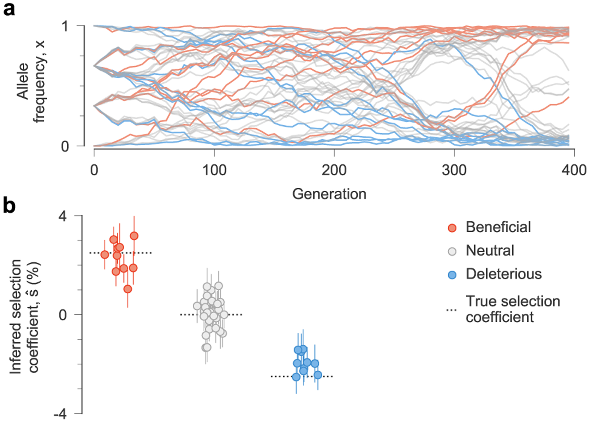
a, Simulated allele frequency trajectories in a model with ten beneficial, 30 neutral and ten deleterious mutant alleles. The initial population is a mix of three subpopulations with random mutations. Selection is challenging to discern from individual trajectories alone. b, Selection coefficients inferred by MPL, presented as mean values ± 1 theoretical s.d. (Methods), are close to their true values. Simulation parameters. L = 50 loci with two alleles at each locus (mutant and WT): ten beneficial mutants with s = 0.025, 30 neutral mutants with s = 0 and ten deleterious mutants with s = −0.025. Mutation probability per locus per generation μ = 10−3, population size N = 103. The initial population is composed of approximately equal numbers of three random founder sequences, evolved over T = 400 generations.
Next, we compared MPL to a panel of state-of-the-art methods of selection inference21,23–26,35. MPL was the most accurate method in terms of both classification accuracy, measured by area under the receiver operating characteristic for classifying mutant alleles as beneficial or deleterious, and in the absolute error in inferred selection coefficients (Fig. 2 and Supplementary Text) across two different simulation scenarios. The first ‘simple’ scenario begins with a homogeneous population. The second ‘complex’ scenario begins with a mixture of five random founder sequences, has stronger selection and a shorter overall time period. Notably, MPL results showed better agreement with the underlying parameters in most individual simulations as well as on average (Extended Data Fig. 2). Due to the simplicity of equation (1), MPL was fastest among the methods that we compared, with a running time roughly six orders of magnitude faster than approaches that rely on iterative Monte Carlo simulations. While these results (Figs. 1 and 2 and Extended Data Fig. 2) are for scenarios without recombination, we note that MPL performs equally well in scenarios with recombination (Extended Data Fig. 3).
Fig. 2 |. MPL compares favorably with state-of-the-art methods.
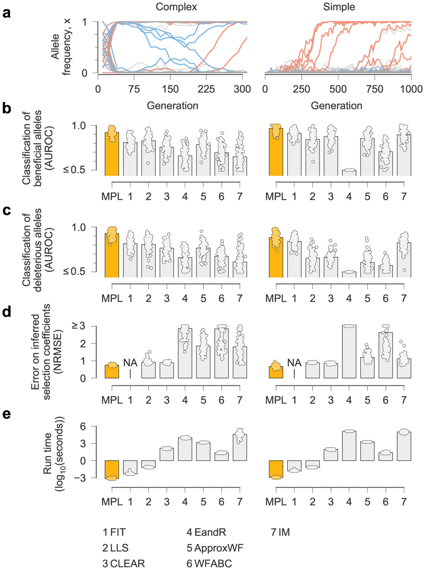
a, We compared the ability of MPL and existing methods to infer selection from simulated test data that was rich with interference patterns and linkage, as shown in representative allele frequency trajectories. To evaluate robustness to finitely sampled data, we selected ns = 100 sequences per time point for inference, with sampling time points separated by Δt = 10 generations. b–e, Performance was evaluated by comparing the successful classification of beneficial (b) and deleterious (c) mutations, error in the estimated selection coefficients (d) and run time (e), averaged over n = 100 replicate simulations with identical parameters. MPL achieves the highest performance in terms of classification and estimation accuracy, and in run time. Note that the frequency increment test (FIT) does not estimate selection coefficients. Simulation parameters. L = 50 loci with two alleles at each locus (mutant and WT): ten beneficial mutants (s = 0.1 for complex, s = 0.025 for simple), 30 neutral mutants (s = 0 for both scenarios) and ten deleterious mutants (s = −0.1 for complex, s = −0.025 for simple). Mutation probability μ = 10−4, population size N = 103. For the complex case, the initial population is composed of equal numbers of five random founder sequences, evolved over T = 310 generations. Recorded trajectories used for inference begin at generation 10. For the simple case, the initial population begins with all WT sequences, evolved over T = 1,000 generations. AUROC, area under the receiver operating characteristic; NA, not applicable; NRMSE, normalized root mean square error.
Patterns of selection in intrahost HIV-1 evolution.
We applied MPL to study the intrahost evolution of HIV-1 and to resolve complex interactions between HIV-1 and the immune system. We analyzed a variety of patient data sets, most of which sequenced half of the HIV-1 genome. Even without omitting invariant sites, the run time for MPL to analyze each data set (containing roughly 2 × 10⁴ variants) was only around 20 min, demonstrating the scalability of our approach. Identifying selective pressures on HIV-1 gives insight into the evolutionary dynamics leading to HIV-1 escape from immune control and the development of bnAbs.
We analyzed 14 patient data sets, initially focusing on a collection of longitudinal HIV-1 half-genome sequence data sets from 13 individuals, where early-phase CD8+ T cell responses were also comprehensively analyzed36, and later on a single data set from an individual who develops bnAbs37,38. MPL is robust to sampling conditions similar to these 14 patient data sets (Supplementary Text and Extended Data Fig. 4). In the first set of 13 individuals, 37.8% of the top 1% most beneficial mutations reported by MPL are nonsynonymous mutations in identified36 CD8+ T cell epitopes (Fig. 3a). This is a 19-fold enrichment in mutations in T cell epitopes compared to expectations by chance (Methods). Here we observe more strongly beneficial escape mutations in subtype B viruses compared to subtype C, which is explained by the larger number of T cell epitopes targeted by individuals infected by subtype B viruses in this data set. Reversions to subtype consensus are also strongly beneficial. Nonsynonymous reversions outside T cell epitopes are 13-fold enriched in this subset. Furthermore, nonsynonymous reversions within T cell epitopes are 320-fold enriched. All enrichment values are highly significant (two-sided Fisher’s exact test P values of <10−30, <10−10 and <10−19, respectively). These findings agree with past studies that have observed strong selection for T cell escape8,9,39 and reversions9.
Fig. 3 |. Patterns of strong selection in intrahost HiV-1 evolution.
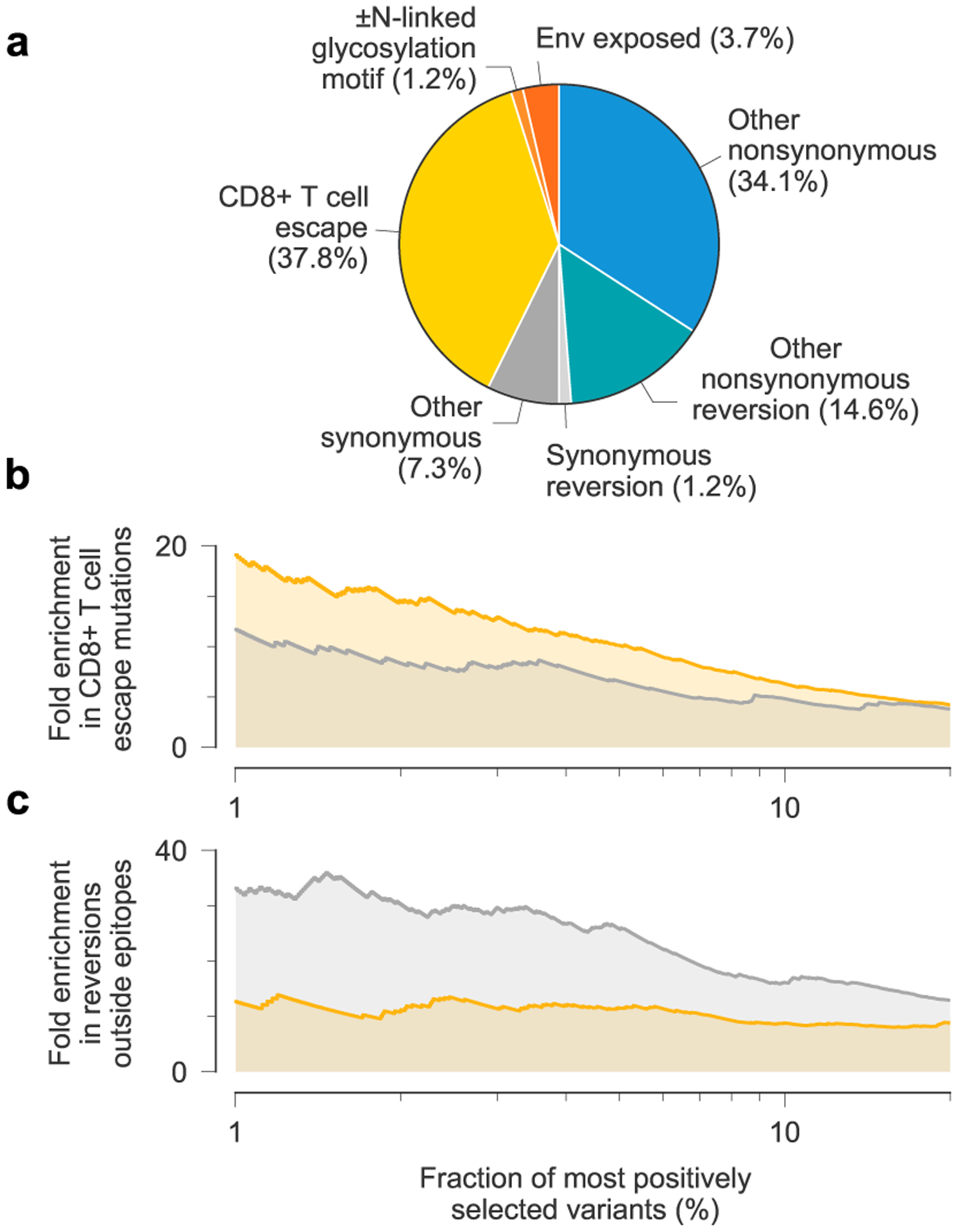
a, Among the top 1% most beneficial variants across individuals, mutations to escape from T cell-mediated immunity are especially common. b, Due to clonal interference between escape mutants, MPL identifies more escape variants to be strongly beneficial than an independent model that ignores genetic linkage. c, In contrast, the independent model estimates an excess in the number of strongly beneficial reversions.
Resolving linkage leads to substantial differences in the magnitude and distribution of selection estimates. MPL places 1.63 times as many T cell escape mutations within the top 1% most beneficial mutations as an independent model that ignores linkage between mutant alleles (Fig. 3b). Conversely, MPL ranks 0.38 times as many nonsynonymous reversions outside T cell epitopes to be strongly beneficial as the independent model does (Fig. 3c). These differences are explained by the joint resolution of genetic linkage effects, including clonal interference.
Quantifying the contribution of linkage to inferred selection.
To dissect the contributions of linkage to estimates of selection, we computed the pairwise effects of each variant i on the inferred selection coefficients for all other variants j (Methods). We defined as the difference between the estimated selection coefficient for variant j using all of the data and the value of when variant i is replaced by the transmitted/founder (TF) nucleotide at the same site, thereby removing the contribution to selection from linkage with variant i. Positive values of indicate that linkage with variant i increases the selection coefficient inferred for variant j (for example, due to clonal interference between them). Negative values indicate that variant i decreases the selection coefficient inferred for variant j (for example, due to hitchhiking). Computing the allowed us to examine the extent to which linkage affects the inference of selection, how these effects were distributed among different genetic variants and how they depend on the distance along the genome between a pair of linked variants.
Distribution of linkage effects on inferred selection.
Our analysis revealed that most observed variants have virtually no effect on estimates of selection at other sites, but a small minority of highly influential variants have dramatic effects (Fig. 4 and Extended Data Figs. 5 and 6). The highly influential variants are often ones that change rapidly in frequency, sweeping through the population and exerting substantial effects on linked sites (Supplementary Fig. 1). Consistent with this observation, 40% of highly influential variants are putative CD8+ T cell escape mutations. This data indicates that some highly influential variants are drivers of selective sweeps.
Fig. 4 |. Maps of strong contributions of linkage to inferred selection.
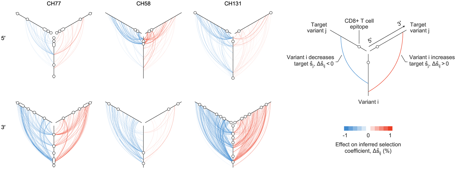
Plot of all large linkage effects on inferred selection coefficients, , for three individuals. One plot is shown for each sequencing region, for each individual. Strong effects of linkage on inferred selection coefficients can span the viral half-genome. Maps of inferred selection for these three individuals are presented in Fig. 5 (CH77, 3′ region), Extended Data Fig. 8 (CH58, 5′ region) and Extended Data Fig. 9 (CH131, 3′ region). Maps of strong contributions of linkage to inferred selection for all individuals are shown in Extended Data Fig. 6.
Our results indicate that the effects of linkage on inferred selection can be highly asymmetrical. That is, a genetic variant i may substantially modify the selection coefficient inferred for variant j, while variant j has little impact on i. Figure 4 shows both cases where linkage effects are asymmetrical and where they are reciprocal.
Association between linkage effects and genomic distance between variants.
While there exist some highly influential variants whose effects span across long genomic distances (Fig. 4 and Extended Data Fig. 6), in most cases, the effects of linkage on estimated selection drop off sharply with increasing distance along the genome (Extended Data Fig. 7a). The largest effects are naturally felt for variants at the same site on the genome, which are in complete competition. Linkage effects on inferred selection are most prominent up to a distance of around 10 bp between variants. Rare, strong linkage effects are noticeably more frequent within distances of around 30 bp, roughly the length of a CD8+ T cell epitope. After this point, additional distance has little influence on the magnitude of linkage effects on inferred selection.
For this data, recombination is expected to contribute to the general decrease in strength of linkage effects on inferred selection with increasing distance along the genome. When two different viruses coinfect the same cell, distinct RNA from each of them can be packaged in new virions. Then, when these virions subsequently infect new cells, HIV-1 can undergo recombination as the reverse transcriptase switches between templates. Estimates show that the effective recombination rate for HIV-1 in vivo is high, around 10−5 per base per generation40,41, which is comparable to the mutation rate. Recombination acts to break up linkage at long distances along the genome, leading to reduced correlations between mutant variants at more widely spaced loci. This effect is clearly evident in the HIV-1 data (Extended Data Fig. 7b). The decay of correlations with distance is smooth, although strong correlations still persist at long ranges. This further indicates the existence of long-range linkage patterns in the data, despite the action of recombination. However, the strongest effects of linkage on inferred selection are comparatively more short-ranged on average, with long-range effects being more punctuated (Extended Data Fig. 7a).
Illustration of the effects of clonal interference on inferred selection.
Viral escape from a T cell response targeting the Nef KF9 epitope in individual CH77 provides a clear example of clonal interference (Fig. 5a). MPL infers strong positive selection for all escape variants. In contrast, when linkage is ignored, escape variants that are lost are inferred to be neutral, and the magnitude of selection for 9040C decreases substantially (Fig. 5b). Experimental tests have shown that most nonsynonymous mutations within CD8+ T cell epitopes are escape mutations, which limit the ability of T cells to kill the mutant form of the virus7. Such mutations are likely to be beneficial to viral replication in vivo. Ignoring linkage thus leads to selection estimates that are qualitatively and quantitatively suspect. We observe similar instances of clonal interference in other epitopes (see Extended Data Figs. 8 and 9 for examples).
Fig. 5 |. estimates of selection coefficients for viral escape mutations must account for clonal interference.
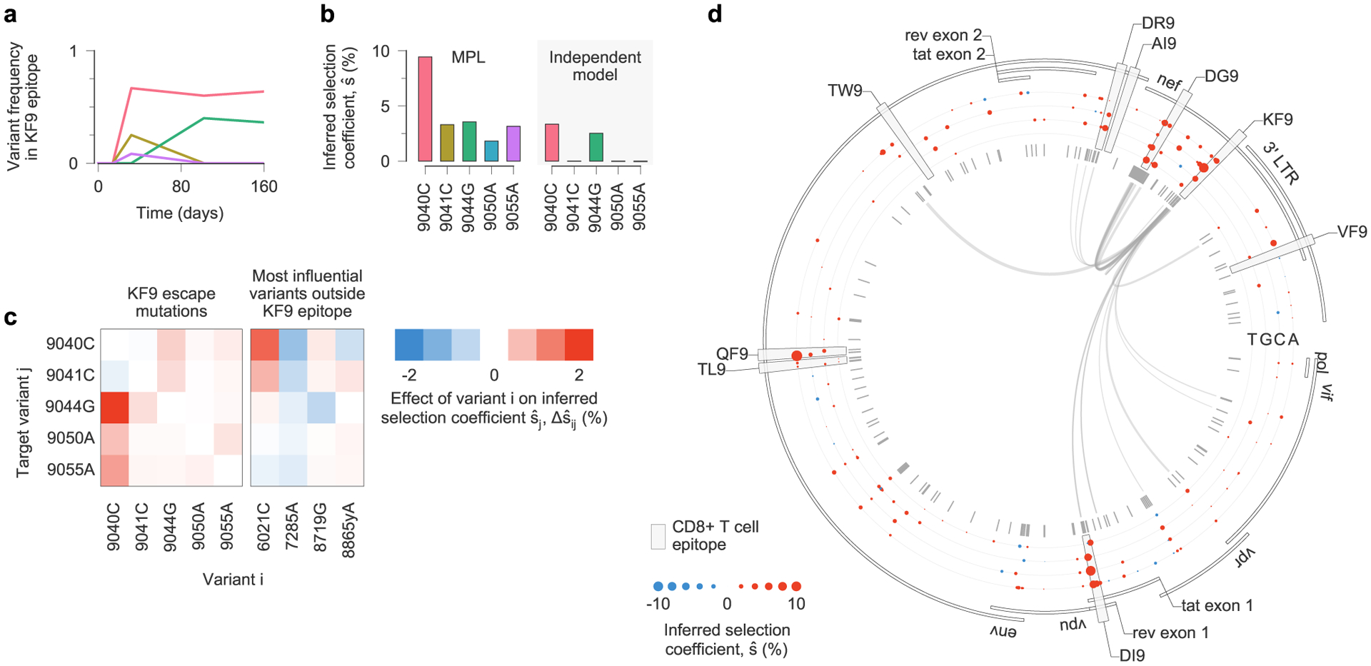
a, Across the viral population, multiple escape mutations appear in the T cell epitope KF9, targeted by individual CH77 and exhibit clonal interference. b, Using the full half-genome-length sequence data as input, MPL infers that all KF9 escape variants are positively selected. In contrast, estimates based solely on the trajectories of individual variants only uncover substantial positive selection for the 9040C and 9044G variants that coexist at the final time point. Furthermore, the independent model infers attenuated estimates of selection because it does not account for competition with other beneficial mutations, including other escape mutations within the same epitope. c, Linkage effects on inferred selection coefficients for KF9 escape mutations. Effects shown here are due to variants within the KF9 epitope and the top four most influential variants outside the KF9 epitope, defined as the variants i for which is the largest. All of these influential variants lie within other T cell epitopes (6021C lies in DI9, 7285A in QF9, 8719G in DR9 and 8865yA in DG9). d, Inferred selection in the HIV-1 half-genome sequence for CH77. Inferred selection coefficients are plotted in tracks. Coefficients of TF nucleotides are normalized to zero. Tick marks denote polymorphic sites. Inner links, shown for sites connected to the KF9 epitope, have widths proportional to matrix elements of the inverse of the integrated covariance (equation (1)). LTR, long terminal repeat.
In the case of KF9, competition between the different escape variants increases the estimated selection coefficient for each of them (Fig. 5c). The interaction between variants 9040C and 9044G, which compete in the viral population at later times, is particularly strong. Inferred selection is also influenced by linkage with other mutations outside the KF9 epitope (Fig. 5c,d). For example, 9040C is inferred to be more beneficial due to its competition with the DI9 escape mutation 6021C. The selection coefficient for 9044G, in turn, is reduced due to positive linkage with 8719G, which is the dominant escape mutation in the nearby Env DR9 epitope.
Modest selection for HIV-1 escape from antibody responses.
The HIV-1 surface protein Env is targeted by antibodies that can block or disrupt infection. Some strongly selected mutations lie in regions of Env that are exposed to antibodies, or in N-linked glycosylation motifs that affect the area of Env that is accessible to antibodies (Fig. 3a). However, these mutations are infrequent compared to others in T cell epitopes. As an example, for the case of CH77, one observes little positive selection in Env outside T cell epitopes (Fig. 5d). Overall, selection for escape from antibody responses appears to be weaker or less frequent than CD8+ T cell-mediated selection.
We asked, therefore, whether strong antibody-mediated selection would be observed in individuals who generate bnAbs. To explore this question, we studied HIV-1 evolution in individual CAP256 who developed the VRC26 lineage of bnAbs37,38. This case is particularly challenging for inference because of a superinfection event 15 weeks after initial infection (Fig. 6a). Superinfection led to intense and complex patterns of linkage as the superinfecting strain recombined and competed with the primary infecting strain (Fig. 6b and Supplementary Fig. 2). For this reason, estimates of selection that ignore linkage are exceptionally poor. Most (six out of 11) of the top 1% most beneficial mutations inferred by the independent model are from the background of the superinfecting strain and are synonymous. In contrast, none of the most beneficial mutations inferred by MPL are synonymous.
Fig. 6 |. complex patterns of selection in HiV-1 env following superinfection in an individual who develops broadly neutralizing antibodies.
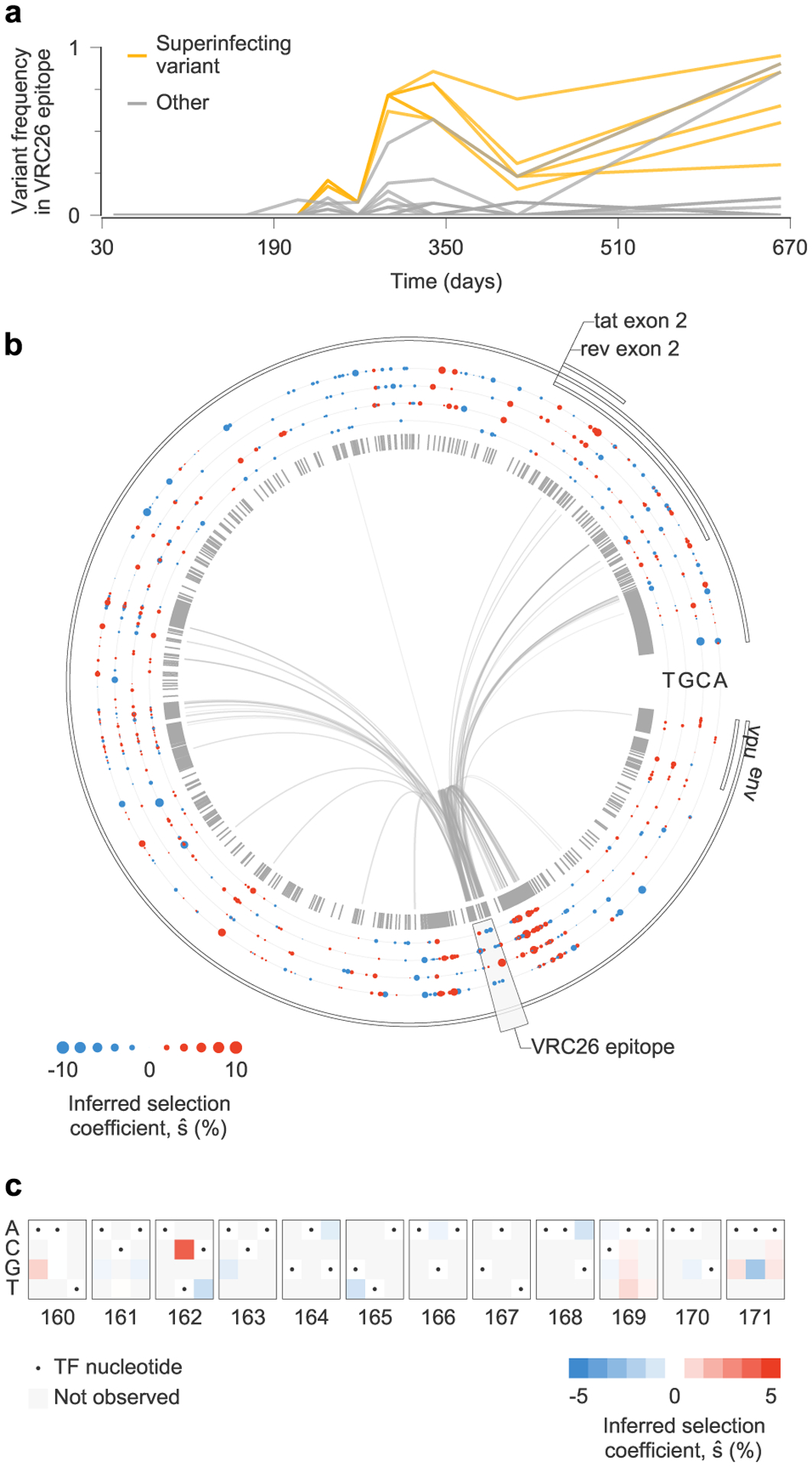
a, Multiple variants, including several from the superinfecting strain of the virus, rise and fall in frequency within the epitope targeted by the VRC26 lineage of antibodies. b, Inferred selection in CAP256 HIV-1 Env sequences. Inferred selection coefficients are plotted in tracks. Coefficients of TF nucleotides are normalized to zero. Tick marks denote polymorphic sites. Inner links, shown for sites connected to the VRC26 epitope, have widths proportional to matrix elements of the inverse of the integrated covariance. Linkage is extensive due to the struggle for dominance in the viral population between the TF, superinfecting and recombinant strains. c, Map of inferred selection within the VRC26 epitope, consisting of codons 160–171 in Env.
We found that selection for known VRC26 resistance mutations37,38 is modest (Fig. 6c). The most strongly selected mutation in the VRC26 epitope region is 6709C in codon 162 in Env, a variant present in the superinfecting strain that completes an N-linked glycosylation motif that is absent from the primary infecting virus. However, this modification makes the virus more sensitive to VRC26 (refs. 37,38). We observed selection against 6717T corresponding to the Env 165L variant in the superinfecting strain. Reversion of this residue to V, the variant in the primary infecting strain, improves resistance to early VRC26 antibodies38. We also observed modest positive selection for nonsynonymous variation at codon 169 in Env (maximum ), where mutations lead to complete resistance to VRC26 lineage antibodies38. Thus, even the most strongly selected resistance mutations fall outside the top 5% most strongly selected mutations in the larger sample of 13 individuals.
Weak selection on the virus for antibody escape may, in fact, facilitate the development of bnAbs. Multiple escape variants, as well as variants that are sensitive to the antibody, can readily coexist for long times when escape is weakly selected. This coexistence increases the diversity of the viral population. Pressure on antibodies to bind to multiple variants can then select for breadth42. Indeed, viral diversification has been observed to precede bnAb development38,43. Stronger pressure on the virus for escape could instead reduce viral diversity due to rapid fixation of beneficial escape variants and the elimination of sensitive ones.
Discussion
We developed an efficient approach to infer the fitness effects of mutations from time series sequence data that accounts for the confounding effects of genetic linkage. MPL successfully infers selection from simulation data, is robust to sampling constraints and it performs favorably compared to state-of-the-art approaches to this problem. Notably, MPL is also fast, easily extending to systems with tens of thousands of genetic variants. Our method is general and should be widely applicable to investigate selection in evolving populations.
Our application of MPL to intrahost HIV-1 evolution demonstrated the importance of resolving linkage due to clonal interference between strongly selected mutations. For some variants, the effects of linkage can extend far across the genome despite frequent recombination. The ability to quantify how linkage affects inferred selection also aids in the interpretability of our results. Our analysis emphasized the central role of T cell escape mutations in HIV-1 evolution, while revealing a modest selection for escape from antibody responses, even in an individual who develops bnAbs. The polyclonality of the antibody response may contribute to weaker overall selection due to conflicting pressures for escape from different antibodies.
The role of CD8+ T cell escape in HIV-1 evolution has also been analyzed in previous studies using techniques and metrics that are distinct from ours. For example, past work estimated selection for T cell escape variants using a simulation-based procedure and a single-locus evolutionary model that does not account for genetic linkage39. T cell escape rates, which are related to (but distinct from) selection coefficients, have also been investigated for HIV-1 in multiple studies. These studies often use specialized differential equation-based models of HIV evolution44–46, and generally do not account for genetic linkage44 or account for it only approximately46–48. Related studies provide evidence for selection for T cell escape by observing increased nonsynonymous variation within T cell epitopes during within-host HIV-1 evolution8,9.
A key distinction of our study, relative to previous studies, is that we provide an unbiased quantification of selection, and how it is affected by linkage, across large stretches of the HIV-1 genome. Our approach is unbiased in the sense that we consider all observed HIV-1 genetic variation, rather than focusing specifically on, for example, T cell escape mutations. While we find that many escape mutations are strongly selected, they still represent a minority of the most beneficial mutations that we observe. Our analysis accounts for and quantifies the interactions between variants observed during within-host HIV-1 evolution, including competition and synergistic interactions within and between CD8+ T cell escape mutations. The ability to quantify selection at the allele level while accounting for linkage effects across large genomic regions is a unique feature of our study.
Our analysis emphasizes the importance of accounting for genetic linkage when inferring selection during HIV-1 evolution. Linkage effects can strongly bias selection inference, despite being dominated by a small subset of variants (Extended Data Fig. 5). Our aggregate analysis shows, for example, that selection for T cell escape is much stronger than would be expected if one were to ignore linkage, while the opposite is true for reversions toward subtype consensus (Fig. 3). The consequences of ignoring linkage are particularly evident for the analysis of CAP256, where, when linkage is disregarded, most variants estimated to have the strongest selection are synonymous. In contrast, all of the most beneficial variants inferred by MPL are nonsynonymous.
Constraints on the type and quality of data necessary for reliable inference place some limitations on the application of our method. While MPL could easily be applied to single-locus data, knowledge of pairwise variant frequencies is needed to disentangle the confounding effects of genetic linkage. Algorithms for estimating genotype distributions, such as those used for haplotype reconstruction in virus populations49 and clone frequency inference in cancer50, could be used to estimate mutant pair correlations in situations where complete information is unavailable. New computational methods that explicitly incorporate temporal information51 would be ideal for reconstructing maps of genetic linkage across time. The continuing development of long-read sequencing technologies will also make pairwise variant frequency data more accessible. As with any inference method, MPL is also limited by the quantity and extent of data available. Genetic variation that lies outside the sequencing region, or undetected genetic alterations (for example, copy number variation) could potentially affect inference results. However, here we found that in HIV-1 evolution data only a small minority of genetic variants strongly affect selection coefficients inferred at other sites (Extended Data Fig. 5). In cases where an important genetic driver is missed, we anticipate that its selective effect will be distributed among linked variants. Limitations in the temporal resolution of sequence data also affect the strength of selection that can reliably be inferred. In particular, selection coefficients for variants that arise and completely fix in between two sampling events are likely to be underestimated.
The evolutionary model that we have used could be extended. While our model is general, it does not yet account for features such as epistasis, time-varying selection or migration. Future work will consider these important questions. The development of practical, efficient algorithms to reveal epistasis in large-scale data remains a particular challenge because the number of parameters to infer grows quadratically with the genome length. Efficient statistical methods, possibly incorporating sparse model selection, will likely be required. In the case of time-varying selection, the selection coefficients that we infer are likely to be similar to the average strength of selection during the time over which that variant was observed. In the case of HIV-1, this may occur, for example, when the magnitude of the immune response against the virus shifts over time. Viral load also undergoes substantial shifts during the course of HIV-1 infection. Although the relationship between viral load and effective population size is complicated52, changes in the number of infected cells could lead to different relative strengths of genetic drift during different stages of infection. Future work will extend MPL to population models with time-varying parameters. While MPL works well with limited sequence data (Extended Data Fig. 1), Bayesian methods to integrate over uncertainty in variant frequency trajectories due to finite sampling could further improve the robustness of our approach.
Our analysis reveals an intriguing link between population genetics and coevolutionary methods53 that have enjoyed great success in predicting protein structure54–56 and fitness57–65 based on sequence information. Coevolutionary methods use a statistical model to capture the low-order moments of the distribution of mutations in a set of sequences, whose parameters can then be related to structure and fitness. So far, there has been no convincing theoretical explanation for the success of coevolutionary methods, or why only the low-order moments are necessary. Here we discovered that, while the evolutionary dynamics of the WF model are defined naturally at the level of genotypes, MPL estimates of fitness only depend on trajectories of the low-order moments of the sequence distribution, at least for the additive fitness landscape that we consider (Methods). Higher-order moments contain no further information about fitness. Energy parameters from Gaussian or standard mean field coevolutionary models53 also have a similar dependence on the inverse of the variant frequency covariance matrix as the selection coefficients inferred by MPL. A mathematical connection between these two frameworks may point to an underlying evolutionary reason for why the low-order statistics used by coevolutionary models are sufficient to capture rich biological information.
Substantial effort in the biomedical sciences is dedicated to identifying the underlying genetic drivers of disease. Notable examples include mutations that promote cancer progression and immune evasion, or mutations that confer drug resistance to bacteria. In the right environment, these mutations confer survival benefits to the pathogens that carry them. However, it can be challenging to separate adaptive mutations from random genetic variation in a complex evolving population. MPL provides a method to infer the fitness effects of individual mutations at large scales even in the face of pervasive genetic linkage. Given the potential pitfalls of ignoring linkage that we have demonstrated, our results call for a greater focus on resolving linkage effects in studies of selection.
Methods
Our method makes use of the diffusion approximation, widely used in population genetics34,66–69, and is a path integral-based framework for statistical inference for a generalized multi-locus model. While familiar in physics70, the path integral approach is less widely used in population genetics, although exceptions exist. Past work has derived path integrals for more specific models and for purposes other than inference31,33, or ignored genetic drift and relied on numerical methods for solution32. The multi-locus model that we use accounts for the effects of selection and mutation, with the key novelty that it also accounts for the effects of linkage, recombination and incomplete temporal sampling. Notably, our approach gives a closed-form solution for the selection coefficients that are most likely to underlie a given evolutionary history.
Evolutionary model.
Our inference approach is based on the standard WF model of population genetics, which describes the stochastic dynamics of an evolving population of N individuals. Each individual is represented by a genetic sequence of length L. The population evolves in discrete, nonoverlapping generations subject to the forces of selection, mutation and recombination. For simplicity, we begin by describing the model with two alleles per locus, WT and mutant. Thus, there are M = 2L unique genotypes. Later, we show that our approach readily generalizes to consider multiple alleles per locus.
The state of the population at a generation t is given by the genotype frequency vector z(t) = (z1(t), …, zM(t)), where za(t) denotes the frequency of individuals with genotype a. Conditioned on z(t), the probability that the genotype frequency vector in the next generation is z(t + 1) is multinomial:34
| (2) |
with
| (3) |
Here fa denotes the fitness of genotype a, and μab is the probability of genotype a mutating to genotype b. For simplicity we will assume at first that the mutation probability μ is the same at all loci, and that the probability of mutating from WT to mutant is the same as that from mutant to WT. In equation (3),
| (4) |
is the frequency of genotype a after recombination. Here r is the probability of recombination per locus per generation, and ψa(t) is the probability that randomly recombining any two individuals in the population results in an individual of genotype a (Supplementary Text). Although equations (3) and (4) appear complex, they have an intuitive interpretation. The first term in equation (3) reflects the fact that fitter individuals reproduce more efficiently and are therefore more likely to be observed in future generations. Mutations, captured through the second term, lead to conversions from genotype a to other genotypes and vice versa. The denominator in equation (3) provides an overall normalization and indicates that relative fitness is important: for a particular genotype to reliably grow in frequency, its fitness should be higher than the average fitness of all individuals in the population. The first term of equation (4) gives the proportion of individuals of genotype a not undergoing recombination, while the second term accounts for the net inward flow due to recombination from all other genotypes to genotype a.
We assume that data consists of sets of genetic sequences obtained from a population at multiple time points tk, k∈ {0, 1, …, K}. For such a population evolving under the WF model, the probability that the genotype frequency vector follows a particular evolutionary path (z(t1), z(t2), …, z(tK)), conditioned on the initial state z(t0), is
| (5) |
This expression is difficult to work with for parameter inference. This is due in part to the high dimensionality of the vector z, which scales exponentially with the length of the genetic sequence. Thus, in most real data sets, the sequence space is dramatically under-sampled. The functional form of equation (2) is also complex.
Our approach circumvents these issues by using two approximations. First, we obtain a simplified version of equation (5) by using a path integral. Path integral expressions for evolutionary models have also been derived under different assumptions in past work31–33, but they have not been widely applied for inference. We also assume that fitness is additive, such that the total fitness of each genotype a is just given by the sum of the selection coefficients si for mutant alleles at each locus i,
Here is 1 if genotype a has a mutant allele at locus i and 0 otherwise. These assumptions will substantially simplify the expression for equation (5).
Path integral for mutant allele frequencies.
In this section we will develop a simplified version of equation (5) defined at the level of allele frequencies rather than genotype frequencies. Later we will demonstrate that, if the fitness effects of mutations are additive as assumed above, this approach will lead to no loss of information for estimating the selection coefficients from data. We begin by using the WF dynamics above, which are defined for genotype frequencies, to compute the expected changes in frequency of mutant alleles. The mutant allele frequency xi at locus i is
Following the assumptions above, and in the WF diffusion limit34, one can show that the probability density for mutant allele frequencies x(t) = (x1(t), x2(t), …, xL(t)) follows a Fokker–Planck equation with a drift vector having entries
| (6) |
and diffusion matrix with entries Cij/N, where
| (7) |
Here xij is the frequency of individuals in the population with mutant alleles at both loci i and j. The drift vector describes the expected change in mutant allele frequencies in time. Note that the last term in equation (6) quantifies linked selection, that is, how the dynamics of mutant allele frequencies are affected by the average genetic background on which they appear. The drift vector should not be confused with genetic drift, the fluctuation in allele frequencies due to the inherent stochasticity of replication, which is instead described by the diffusion matrix. The diffusion matrix is simply the covariance matrix of mutant allele frequencies divided by the population size N. It therefore depends on the double mutant frequencies xij, but we will use the shortened notation Cij(x(t)) for brevity.
Applying standard methods from statistical physics70, the Fokker–Planck equation can be converted into a path integral that quantifies the probability density for ‘paths’ of mutant allele frequencies (x(t1), x(t2), …, x(tK)). This expression will allow us to efficiently estimate the parameters that are most likely to have generated a specific path (Supplementary Text). The probability for a path is
| (8) |
where Δtk = tk+1 − tk. In the language of physics, is referred to as the action. The population size N is analogous to the inverse temperature in statistical physics. The action penalizes deviation of the change in mutant frequencies between generations from the expectation given by the drift vector at the previous generation. This is normalized by the diffusion matrix, which quantifies the magnitude of typical changes in mutant frequencies due to random replication alone (that is, genetic drift). The path integral equation in (8) follows the Itô convention.
MPL estimate of the selection coefficients.
Given an observed path of mutant allele frequencies, we can use Bayesian inference to determine the maximum a posteriori selection coefficients corresponding to the data, assuming that the population size N and mutation probability μ are known. In practice, our data consists of sets of genetic sequences obtained from a population at multiple time points tk, k ∈ {0, 1, …, K}. These sequences can be used to compute the path of mutant allele frequencies (x(t0), x(t1), …, x(tK)) as well as the double mutant frequencies xij(tk), which also appear in equation (8). We will assume that the observed mutant allele frequencies are equal to the true ones, which simplifies the inference procedure. Our tests indicate that our results are robust to errors in the frequencies due to finite sampling (Extended Data Fig. 1). Future work will relax this assumption.
In total, the posterior probability of the selection coefficients s = (s1, s2, …, sL) given the observed path (x(t0), x(t1), …, x(tK)) is
| (9) |
where is the probability of the path (given by equation (8), but extended to arbitrary sampling times as shown in Supplementary Text) and Pprior(s) is the prior probability for the selection coefficients. Equation (9) is a complicated expression of the mutant allele frequencies. However, solving for the selection coefficients that maximize the posterior probability is straightforward because equation (8) is a Gaussian function of the selection coefficients. Taking Pprior(s) to be Gaussian with mean zero and covariance matrix σ2I, where I is the identity matrix, the selection coefficients that maximize equation (9) are given by equation (1), with
| (10) |
Collectively, this gives
| (11) |
where γ = 1/Nσ2. We refer to this as the MPL estimate of selection coefficients. Because of the Gaussian form of equation (9), the maximum a posteriori estimates of the selection coefficients are the same as their posterior means. The theoretical covariance in the inferred selection coefficients can also be computed from equation (9), which is given by .
Equation (11) can be readily interpreted. Let us start by considering the vector term in the ‘numerator’ of equation (11) that multiplies the matrix inverse. Here the first terms quantify how the frequency of each mutant allele has changed between the initial and final generations. Naturally, alleles that increase in frequency over time are more likely to be beneficial. The remaining terms quantify the integrated mutational flux, that is, population flow from mutant to WT (or vice versa) due to mutation. Net mutational flux from mutant to WT is also associated with higher fitness for the mutant allele. This is because this indicates that the mutant state maintained higher frequency than the WT over the trajectory, despite the force of mutation that drives the frequencies toward the same value. Together, these terms in the numerator of equation (11) determine whether a mutant allele is inferred to be beneficial or deleterious, at least when the off-diagonal elements of the matrix that it multiplies are zero.
While the numerator of equation (11) roughly determines the sign of selection, the denominator determines the strength of the inferred selection coefficient. Let us refer to as the integrated covariance matrix, Cint. From equation (7) we see that the entries of Cij(x(t)) are small when the mutant frequency is near the boundaries (0 or 1). Thus, the dominant contribution to the integrated covariance matrix comes from points on the path where the mutant frequency is far from the boundaries. If selection is strong, so that the mutant allele is much fitter than the WT (or vice versa), then we expect that a large portion of the path will be spent with the mutant allele frequency close to the boundary. In such cases the diagonal part of the integrated covariance will be small, and we correctly infer strong selection. The prior distribution for the selection coefficients simply adds a constant to the diagonal of the integrated covariance, which both shrinks selection estimates toward zero and ensures that the matrix is invertible. The off-diagonal terms of the integrated covariance matrix capture linkage effects, that is, how much of the change in the mutant frequency at a locus can be attributed to the average sequence background on which the mutant appears.
The effect of recombination is notably absent from equation (11). While the evolutionary model (equations (3) and (4)) incorporates recombination, the recombination term cancels out during the genotype to allele transformation, and thus the MPL estimate is independent of the recombination probability r under the additive fitness model assumed here (Supplementary Text). While recombination certainly affects the types of evolutionary history that are likely to be observed (by reducing linkage disequilibrium, see Extended Data Fig. 3), it does not affect the selection coefficients that we estimate conditioned on a particular evolutionary history.
Equivalence of genotype- and allele-level analyses.
In the preceding section we derived an estimate for the selection coefficients most likely to have generated an observed evolutionary path. To do this we used an expression for the likelihood of a path of mutant allele frequencies that depended on the mutant frequencies xi(t) and their pairwise correlations xij(t), but not on higher-order correlations of the full genotype distribution. However, the WF dynamics is defined at the level of genotypes.
It can be shown that the use of equation (8) does not result in any loss in information beyond the approximations inherent in the WF diffusion limit. In the WF diffusion limit, the same steps as those applied to derive equation (8) can be performed for the genotype frequencies (Supplementary Text). This results in a path integral expression that quantifies the probability density of genotype frequency paths. As in the allele-level analysis, the estimated selection coefficients are those that maximize
where is the probability density of the genotype frequency path. The full expression is more complicated, and less transparent, than the allele-level equivalent. Nonetheless, one can show that the expression for the selection coefficients that maximize the posterior probability above is exactly the same as equation (11). Full details of this derivation are given in the Supplementary Text. This result is important because it shows that, following the assumptions of the WF diffusion limit and assuming that the fitness effects of mutations are additive, higher-order mutational correlations contain no further information about the fitness effects of mutations.
Extension to multiple alleles per locus and asymmetric mutation probabilities.
The MPL framework extends readily to models with ℓ alleles per locus, as well as asymmetric mutation probabilities. Let xi,α(t) denote the frequency of allele α at locus i at generation t, and denote μαβ as the mutation probability per locus from allele α to allele β. Now, the trajectory of allele frequency vectors is (x(t0), x(t1), …, x(tK)), where x(tk) = (x1,1 (tk), x1,2(tk), …, x1,ℓ(tk), x2,1(tk), …, xL,ℓ(tk))
Following parallel arguments to before (Supplementary Text), the MPL estimate of the selection coefficient for allele α at locus i is
| (12) |
where γ = 1/Nσ2 as before. Off-diagonal entries of the covariance matrix C(x(tk)) are given by
where xij,αβ(tk) is the frequency of sequences with alleles α and β at loci i and j, respectively, at time tk.
Simulation data.
We implemented the WF model with discrete generations in Python. Briefly, we evolved populations of sequences according to equation (2) over T = tK generations, recording the entire evolutionary history. To mimic finite sampling in real data, we randomly selected ns sequences from the population to be used for analysis every Δt generations. For example, if ns = 100 and Δt = 10, we would select 100 sequences at random from the population every ten generations for the purposes of estimating selection coefficients. In cases where we show data from multiple trials, this data is obtained from independent simulations with the same underlying parameters. The initial population and simulation parameters are described in the figure captions. For MPL, we computed the single xi and double xij mutant frequencies from the sampled sequences and used them to infer the selection coefficients with equation (11). We used this program to record 100 evolutionary histories each for three different choices of the underlying parameters. Parameter values are detailed in Extended Data Figs. 1 and 2. For all simulations we assumed only two alleles per site. The simulation code, code for analysis and original simulation data are contained in the GitHub repository.
Other time series inference methods.
The independent model that we compared MPL against in the main text is a single-locus variant of MPL in which the off-diagonal elements of the integrated covariance matrix are set to zero.
The seven additional time series-based inference methods that we compared MPL against are frequency increment test (FIT)21, linear least squares (LLS)25, composition of likelihoods for evolve and resequence experiments (CLEAR)35, evolve and resequence (EandR)28, approximate Wright–Fisher (ApproxWF)24, Wright–Fisher approximate Bayesian computation (WFABC)23 and Illingworth and Mustonen’s method (IM)26. Where available, we used the scripts provided by the authors. Some of these methods required preprocessing of the time series data to obtain valid estimates of selection coefficients. See Supplementary Text for details on implementation and data processing.
Patient cohort.
We studied HIV-1 sequence data obtained from 14 individuals recruited under the CHAVI 001 and CAPRISA 002 studies in the United States, Malawi and South Africa. The locations of CD8+ T cell epitopes were experimentally36 or computationally61 determined in 13 of the 14 individuals. In the remaining individual, CAP256, experimental studies identified the VRC26 family of antibodies and mapped the epitope location on Env38.
HIV-1 sequence data.
Multiple sequence alignments of HIV-1 nucleotide sequences for all individuals were obtained from the Los Alamos National Laboratory (LANL) HIV Sequence Database (www.hiv.lanl.gov; accessed 19 October 2018). Sequences labeled as problematic were not downloaded. For the 13 individuals with identified T cell epitopes, sets of 3′ and 5′ half-genome sequences were obtained, which were approximately 4,500 bp in length. Only Env sequences were available for CAP256 (approximately 2,500 bp in length). All sequences were aligned with the HXB2 reference sequence (GenBank accession number K03455) for numbering, and with subtype consensus sequences to determine reversions, using the LANL HIVAlign tool71. A summary of the data is given in Supplementary Table 1.
For each patient data set, except for CAP256, the TF virus was deduced from single genome amplification and sequencing of plasma virus taken in acute infection close to peak viremia36. For CAP256, the transmitted founder sequence was not determined, and analysis started with sequences obtained 42 d after infection38. In our analysis, we defined the TF nucleotide at each site based on TF sequences in the LANL HIV Sequence Database. In cases where the TF sequence was not available, we used the most frequently observed nucleotide at each site at the earliest sequencing time point.
Accurately inferring selection requires balancing the benefits of additional data versus the potential drawbacks of statistical noise due to, for example, small numbers of available sequences or large time gaps. For this reason, we applied various selection criteria to limit the influence of noise and other artifacts in the data.
Maximum number of gaps.
Sequences with large numbers of gaps may have large deletions or sequencing regions that only partly overlap with the region of interest. We therefore removed sequences with >200 gaps in excess of the subtype consensus sequence from the analysis.
Maximum gap frequency.
Rare insertions, which would appear in the data as sites with high gap frequencies, may represent misalignments. We conservatively removed sites with >95% gaps from our analysis.
Minimum number of sequences.
Additional time points are helpful for identifying selection, but variant frequencies at time points with small numbers of sequences are poorly constrained by the data. This finite sampling noise may make it difficult to reliably infer selection. We therefore dropped time points where fewer than four sequences were observed from our analysis.
Maximum time gap.
Large time gaps can degrade performance if they cause us to miss evolutionary dynamics that are relevant for inferring selection. Here we dropped time points that were separated by >300 d from the last included time point.
Imputation of ambiguous nucleotides.
To include sequences that contain some ambiguous nucleotides in our analysis, we imputed ambiguous nucleotides by replacing them with the most frequently observed nucleotide at the same site from that patient. Imputations were also constrained by the identity of the ambiguous nucleotide. For example, an R would be replaced by either A or G, depending on which nucleotide was more frequently observed at that site in the same patient.
For all of these exclusion criteria, different thresholds could reasonably have been chosen. Extended Data Fig. 10 shows that the selection coefficients that we infer are robust to the specific data processing choices that we have made.
In the course of data processing we also determined the number of open reading frames in which each substitution was nonsynonymous, whether it occurred within an identified CD8+ T cell epitope that was actively targeted during the time for which sequence samples were available, whether it occurred within the exposed surface of Env (using surface residues as identified in ref. 63), and whether it may have plausibly affected Env glycosylation by completing or disrupting an N-linked glycosylation motif. These analyses were performed using custom Python scripts available in the GitHub repository.
Variant indices were labeled relative to the standard HXB2 reference sequence of HIV-1. Insertions relative to HXB2 are labeled with lowercase alphabetical indices per standard conventions72. For example, if three nucleotides were inserted relative to HXB2 after site 1, these would be labeled 1a, 1b and 1c, respectively.
Enrichment analyses.
We used fold enrichment values to determine the relative excess or lack of particular types of mutation among the HIV-1 variants that were inferred to be the most beneficial. For a given set of Nsel selected mutations (for example, corresponding to the top 1% most beneficial), we computed the number nsel of these mutations that have a particular property. This may represent, for example, the number of nonsynonymous mutations within identified CD8+ T cell epitopes, or the number of nonsynonymous reversions. The ratio nsel/Nsel then represents the fraction of the selected mutations having the specified property. This number was compared with nnull/Nnull, where Nnull is the total number of non-TF variants across all individuals and sequencing regions of the HIV-1 genome and nnull is the number of these variants that share the specified property.
The fold enrichment of the selected set for a specified property is then naturally defined as (nsel/Nsel)/(nnull/Nnull). A fold enrichment value greater than one indicates a larger proportion of mutants in the selected set that have the given property than expected by chance, while a value less than one indicates a smaller proportion than expected by chance.
Selection inference with MPL.
We implemented the MPL method as described above in C++ and applied it to infer selection coefficients from the HIV-1 sequence data and from simulations. The original code used for inference is included in the GitHub repository. For the HIV-1 data, we assumed a regularization strength of γ = 5. We also used mutation probabilities estimated in ref. 73. as input. Mutation probabilities to and from gap states, representing deletions and insertions, respectively, were assumed to be very small (μ = 10−9). For the simulated data, we used a smaller regularization strength of γ = 1 due to the greater sampling depth.
For time intervals Δt ≫ 1, naïve evaluation of Cint and μfl may give results that are inconsistent with more realistic, smoothly varying allele frequencies. For example, if a variant rises from frequency zero to a nonzero frequency in the final time step, the diagonal part of the integrated covariance Cint from equation (10) would formally be zero for this variant. To increase robustness and avoid unnatural covariance and flux terms, we assumed that the true underlying allele frequency trajectories were piecewise linear and replaced the sums over time in equation (12) with integrals. Following the assumption of piecewise linearity, these integrals can be computed analytically. Specifically, the contribution of the mutational term to the numerator is then
the diagonal terms of the integrated covariance matrix are
and the off-diagonal terms of the integrated covariance matrix are
After selection coefficients were inferred, we normalized them such that the TF (HIV-1) or WT (simulation) allele had a selection coefficient of zero.
Calculation of effects of linkage on inferred selection.
Due to the inverse of the integrated covariance matrix in equation (11), the selection coefficients estimated by MPL are affected by linkage. To quantify the effects of linkage on inferred selection during HIV-1 evolution, we computed the pairwise effects of each variant i on selection for other variants j, as described in the main text. Here, for ease of notation, each effective index i or j represents a single non-TF nucleotide at a particular site on the genome. That is, the indices incorporate both the label for the locus and for the allele.
To compute , we iteratively select each nucleotide at each site, which together are represented by the index i, and generate a modified version of the sequence data in which variant i is replaced by the TF nucleotide at the same site. In this way, linkage between the masked variant i and all other variants j is eliminated. We then infer the selection coefficients again for all variants j using the data where variant i has been replaced by TF, denoted as . Then we define
Positive values of thus indicate that linkage with variant i increases the selection coefficient inferred for variant j. This may be due, for example, to clonal interference between variants i and j. Negative values indicate that variant i decreases the selection coefficient inferred for variant j. This may occur, for example, if variant j hitchhikes on a beneficial genetic background that includes variant i.
Statistics and reproducibility.
Details of enrichment analysis are given in Methods. The P values were calculated using the two-sided Fisher’s exact test. Simulation results in Fig. 2 and Extended Data Figs. 1–4 were computed on 100 evolutionary histories each obtained from an independent Monte Carlo run. The theoretical covariance in the inferred selection coefficients can be computed from equation (9), which is given by . In Fig. 1 and Extended Data Fig. 1b, we show theoretical standard deviations on the inferred selection coefficients, computed by the square root of the diagonal entries of .
Extended Data
Extended Data Fig. 1 |. MPL accurately recovers selection coefficients from complex simulated evolutionary trajectories.
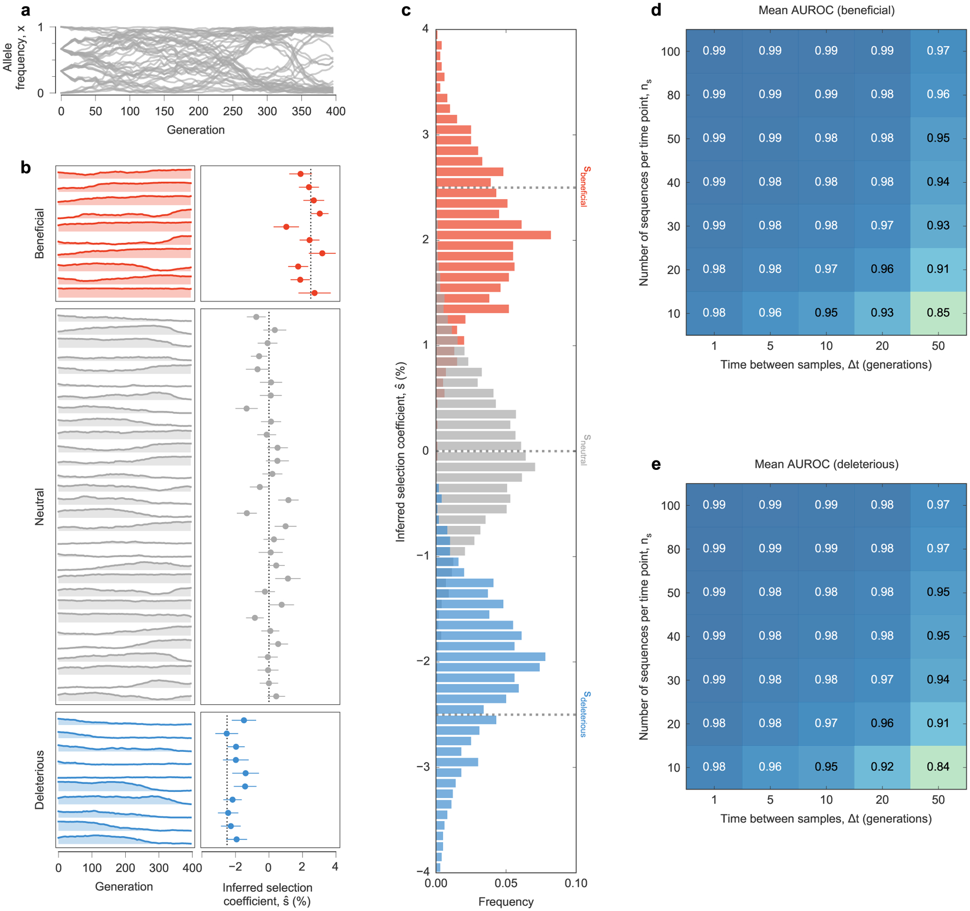
a, Trajectories of mutant allele frequencies over time exhibit complex dynamics in a WF simulation with a simple fitness landscape. b, Separate views of individual trajectories for beneficial, neutral, and deleterious mutants (left panel) and inferred selection coefficients (right panel) for a single simulation run. Note that many neutral mutations exhibit temporal variation similar to beneficial or deleterious mutations. MPL estimates the underlying selection coefficients used to generate these trajectories, presented as mean values ± one theoretical standard deviation, and distinguishes between beneficial, neutral, and deleterious mutations, using Eq. (11). Dashed lines mark the true selection coefficients. c, Distributions of selection coefficient estimates across n = 100 replicate simulations with identical parameters in the special case of perfect sampling. MPL is also robust to finite sampling constraints, accurately classifying beneficial (d) and deleterious (e) mutants even when the number of sequences sampled per time point ns is low, and the spacing between time samples Δt is large. Simulation parameters. L = 50 loci with two alleles at each locus (mutant and WT): ten beneficial mutants with s = 0.025, 30 neutral mutants with s = 0, and ten deleterious mutants with s = −0.025. Mutation probability μ = 10−3, population size N = 103. Initial population composed of approximately equal numbers of three random founder sequences, evolved over T = 400 generations.
Extended Data Fig. 2 |. MPL improves selection inference for simulated data sets.
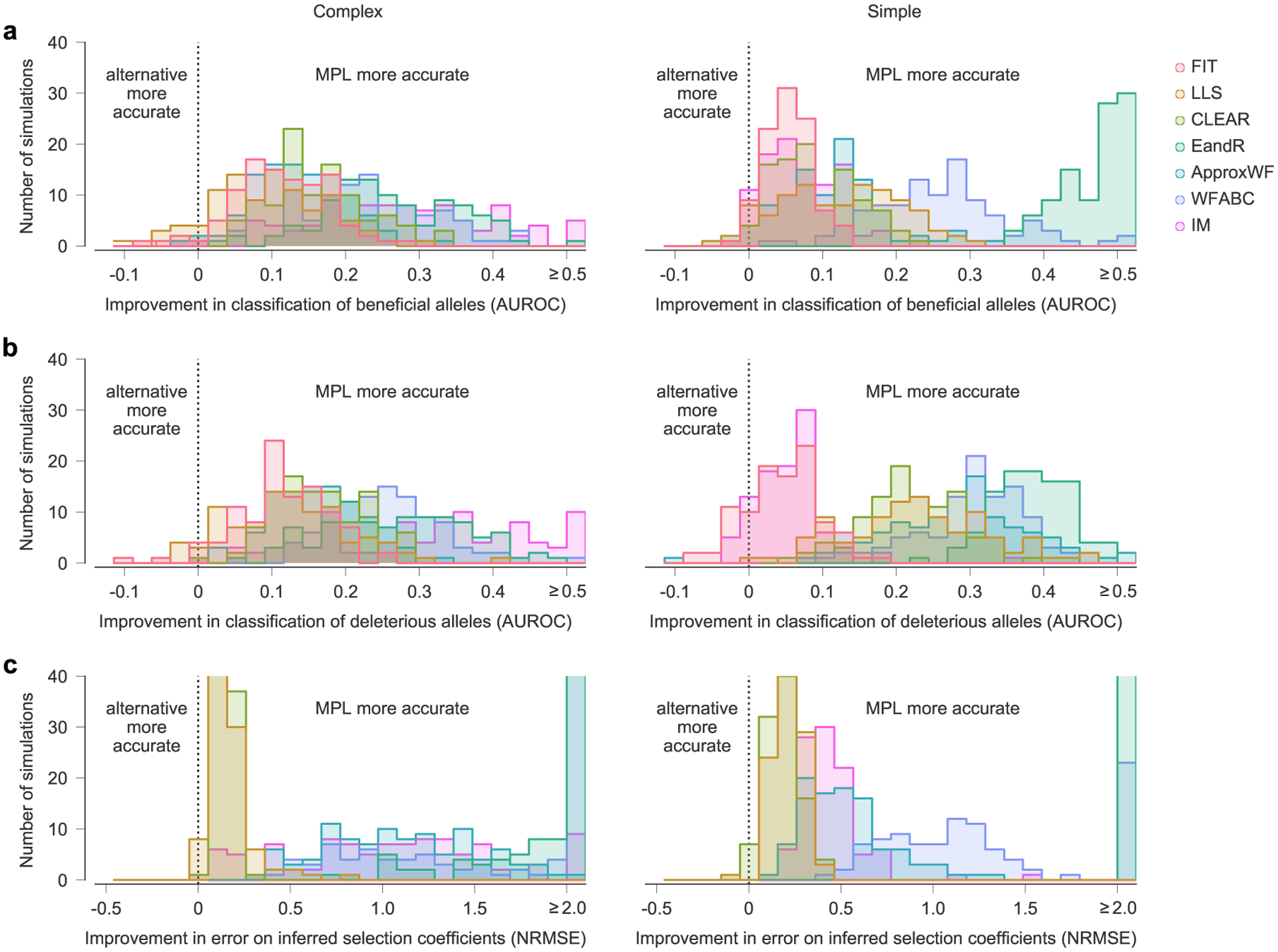
In Fig. 2, we showed the performance of MPL and existing methods on simulated test data, averaged over n = 100 replicate simulations with identical parameters. Here we show the improvement of MPL over existing methods for the classification of beneficial (a) and deleterious (b) mutations, and for the error in the estimated selection coefficients (c), for each individual simulation. Selection is more difficult to infer in some simulated data sets, but results from MPL show better agreement with the true parameters in the vast majority of simulations. Simulation parameters. L = 50 loci with two alleles at each locus (mutant and WT): ten beneficial mutants (with s = 0.1 for complex, s = 0.025 for simple), 30 neutral mutants (s = 0 for both scenarios), and ten deleterious mutants (s = −0.1 for complex, s = −0.025 for simple). Mutation probability μ = 10−4, population size N = 103. For the complex case, the initial population is composed of equal numbers of five random founder sequences, evolved over T = 310 generations. Recorded trajectory used for inference begins at generation 10. For the simple case, the initial population begins with all WT sequences, evolved over T = 1000 generations.
Extended Data Fig. 3 |. MPL performs well in the presence of recombination.

a, Classification performance of MPL is robust to variation in per locus recombination probability, r. Results are shown for n = 100 independent Monte-Carlo runs. The lower and upper edge of the boxplot correspond to the 25th to 75th percentiles, the bar corresponds to the median while the top and bottom whiskers show the maximum and minimum value within 1.5× the interquartile range from the boxplot. Linkage effects in the data decrease as the recombination probability increases. As a measure of the linkage disequilibrium in the data, we plot the histograms (b) of the covariance (xij − xixj) of mutant allele frequencies integrated over time (300 generations) for a range of recombination probabilities. The number of mutant pairs with strong pairwise covariance values decrease with increasing values of r, indicating lower linkage disequilibrium. Simulation parameters. Same as those of simple scenario used in Fig. 2, that is, L = 50 loci with two alleles at each locus (mutant and WT): ten beneficial mutants (s = 0.025), 30 neutral mutants (s = 0), and ten deleterious mutants (s = −0.025). Mutation probability μ = 10−4, population size N = 103, r = {0, 10−5, 10−4, 10−3}. The initial population begins with all WT sequences, evolved over T = 300 generations.
Extended Data Fig. 4 |. Performance of MPL on data with HiV-1-like sampling profiles.
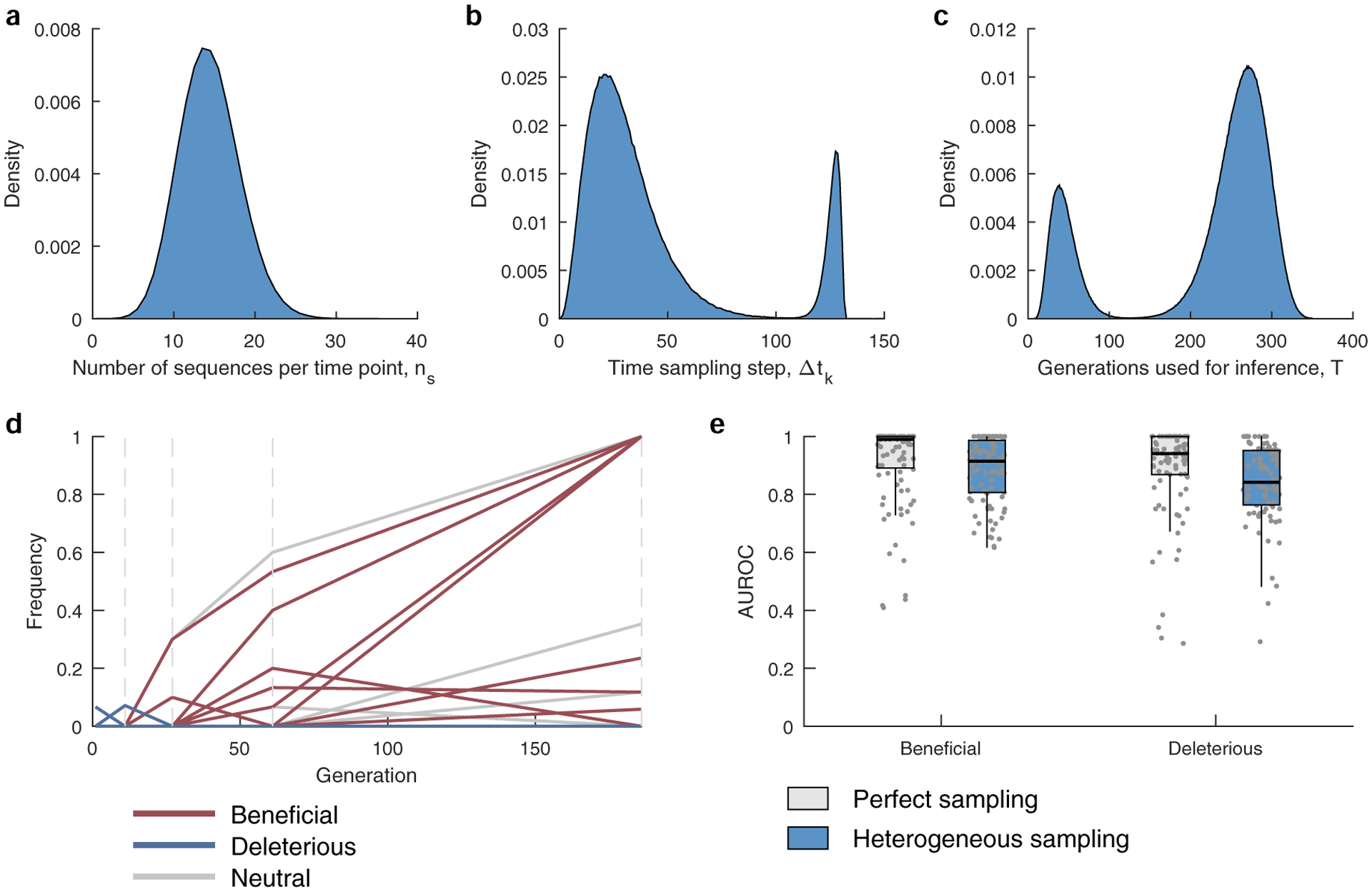
a, The number of sequences per time point ns are drawn from a binomial distribution with n = 1000 and p = 0.0139, with the same mean as that of the HIV data. b, The time between samples is drawn from a mixture of two gamma distributions f(x;k,θ), where k and θ are the shape and scale parameters. The mixture distribution has the form w1 × (f(x;k1,θ1) + m1) + w2 × (f((k2θ2 + m2 − x);k2,θ2) + m2) where m1 = 0, m2 = 120, are constants added to shift the mean, k1 = 3.5, k2 = 3, θ1 = 8.4, θ2 = 2, while w1 = 0.87, and w2 = 0.13 are the mixing weights. The parameters were chosen to mimic the distribution of the time between samples of the HIV data analyzed in the manuscript (Supplementary Table 1). c, The number of generations used for inference is also drawn from a mixture of two gamma distributions, having the form given above and with parameters k1 = 5.5, k2 = 15, θ1 = 7.2, θ2 = 8, m1 = 5, m2 = 143, w1 = 0.21, and w2 = 0.79. The parameters were chosen to mimic the distribution of the trajectory lengths of the HIV data analyzed in the manuscript (Supplementary Table 1). d, A typical sampled trajectory of allele frequencies: beneficial (red), deleterious (blue) and neutral (gray). Dashed lines indicate the sampling time-points. e, The AUROC performance of identifying beneficial and deleterious selection coefficients under perfect and heterogeneous sampling scenarios. Results are evaluated for those sites that are polymorphic in the heterogeneous sampling case. Results are shown for n = 100 independent Monte-Carlo runs. The lower and upper edge of the boxplot correspond to the 25th to 75th percentiles, the bar corresponds to the median while the top and bottom whiskers show the maximum and minimum value within 1.5× the interquartile range from the boxplot. Simulation parameters: population size N = 1000, L = 50 loci with two alleles at each locus (mutant and WT), ten beneficial mutants with selection coefficients s uniformly distributed over the range [0.075, 0.125], 30 neutral mutants with s = 0, and ten deleterious mutants with selection coefficients uniformly distributed over the range [−0.125, −0.075], mutation probability per site per generation μ = 10−4, and recombination probability per site per generation r = 10−4.
Extended Data Fig. 5 |. Most genetic variants have little effect on inferred selection at other sites, but a small minority have strong effects.
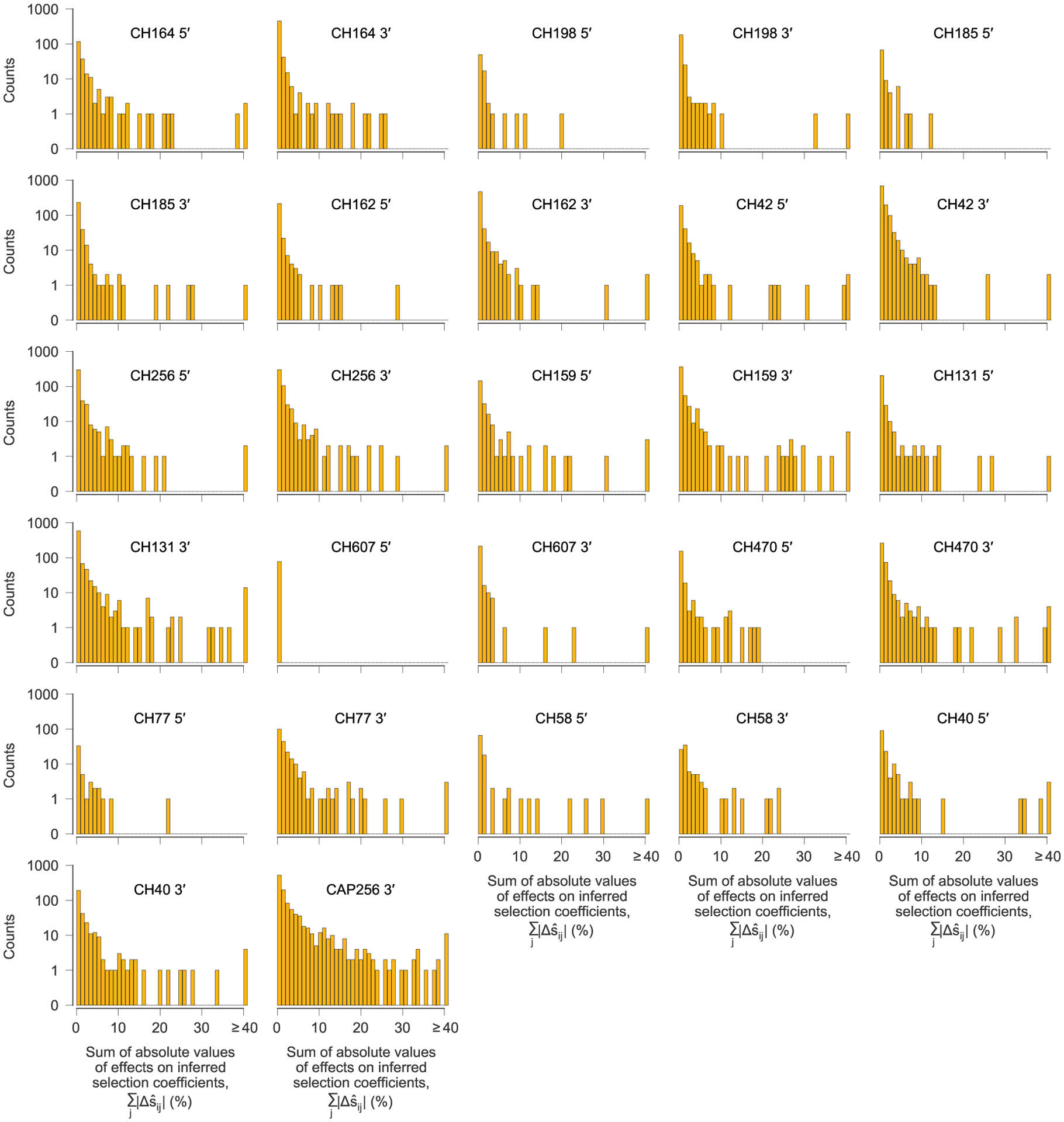
After computing the pairwise effects of each variant i on the inferred selection coefficient for each other variant j, referred to as the target, we summed the absolute value of the values over all target variants j to quantify the influence of each variant i on selection at other sites. One histogram is shown for each sequencing region, for each individual. For the vast majority of variants, the total effect on selection at other sites is near zero. However, a small minority have strong effects. We defined a variant to be ‘highly influential’ if the sum of the absolute values of the over all targets j was larger than 0.4 (=40%).
Extended Data Fig. 6 |. Variants that strongly influence inferred selection at other sites often act across large genomic distances.
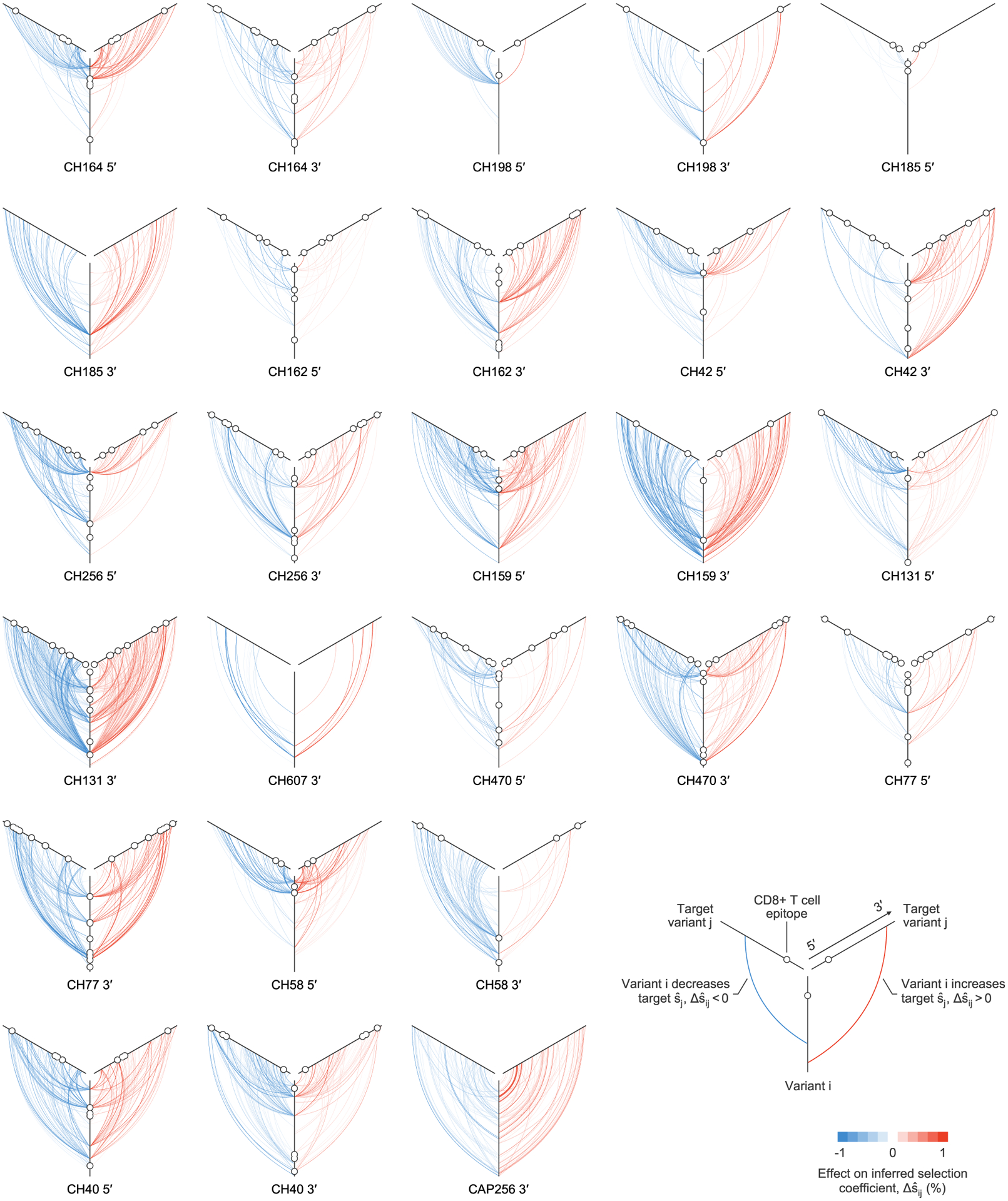
Plot of all linkage effects on inferred selection coefficients for which . One plot is shown for each sequencing region, for each individual. These strong effects of linkage on inferred selection coefficients can act at long range across the genome. Approximately 40% of highly influential variants, characterized by strong effects on inferred selection at other sites, lie within identified CD8+ T cell epitopes. The 5′ region for individual CH607 is not shown because no values are larger than the cutoff.
Extended Data Fig. 7 |. For most variants, effects on inferred selection coefficients for other variants, and linkage disequilibrium, are stronger at smaller genomic distances.
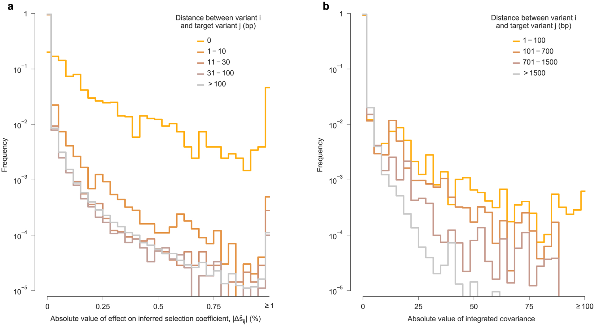
a, Histogram of the absolute value of linkage effects on inferred selection coefficients for other variants , divided into subgroups based on the distance along the genome between variant i and target variant j. Consistent with intuition, the large effects on inferred selection coefficients occur most frequently for different variants that occur at the same site on the genome (that is, distance equal to zero). ‘Interactions’ between such variants are necessarily perfectly competitive because only a single nucleotide is allowed at each position in the genetic sequence. For most variants, stronger linkage effects on inferred selection coefficients are more frequently observed for other variants within a distance of ten base pairs (bp). Large linkage effects for pairs of variants within a distance of 30 bp, the approximate length of a linear T cell epitope, occur appreciably more frequently than for pairs of variants at greater genomic distances. However, there is little difference in the distribution of linkage effect sizes for pairs of variants that are between 31 bp and 100 bp apart compared to pairs of variants that are more than 100 bp apart. Nonetheless, some strong linkage effects on inferred selection are observed at long genomic distances (see Fig. 4 and Supplementary Fig. 5). b, Linkage disequilibrium, measured by the absolute value of the off-diagonal entries of the integrated allele frequency covariance matrix, Cint. Like the , linkage decays along with the distance between variants along the genome. However, we note that linkage disequilibrium values in general appear to be more long-ranged.
Extended Data Fig. 8 |. estimates of selection coefficients in a simple example of clonal interference.
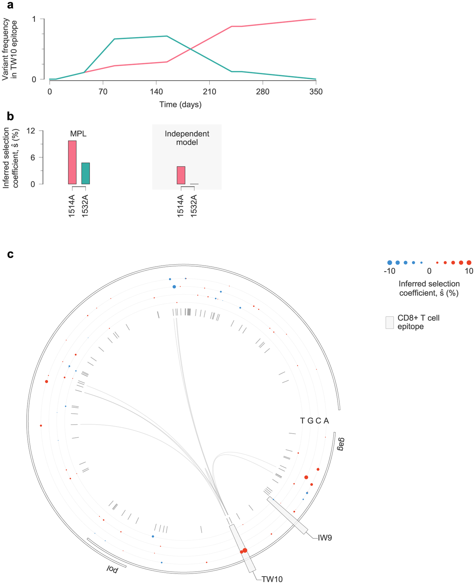
a, Two escape mutations arise in the TW10 epitope targeted by individual CH58 and compete for dominance. b, MPL infers that both TW10 escape variants are positively selected. Estimates based on trajectories of individual variants only infer substantial positive selection for the 1514A variant that fixes. The magnitude of selection inferred with the independent model is also smaller than that inferred by MPL. c, Inferred selection in the HIV-1 5′ half-genome sequence for CH58. Inferred selection coefficients are plotted in tracks. Coefficients of transmitted/founder nucleotides are normalized to zero. Tick marks denote polymorphic sites. Inner links, shown for sites connected to the TW10 epitope, have widths proportional to matrix elements of the inverse of the integrated covariance. Linked sites affect selection estimates within the epitope.
Extended Data Fig. 9 |. estimates of selection coefficients in a complex example of clonal interference.
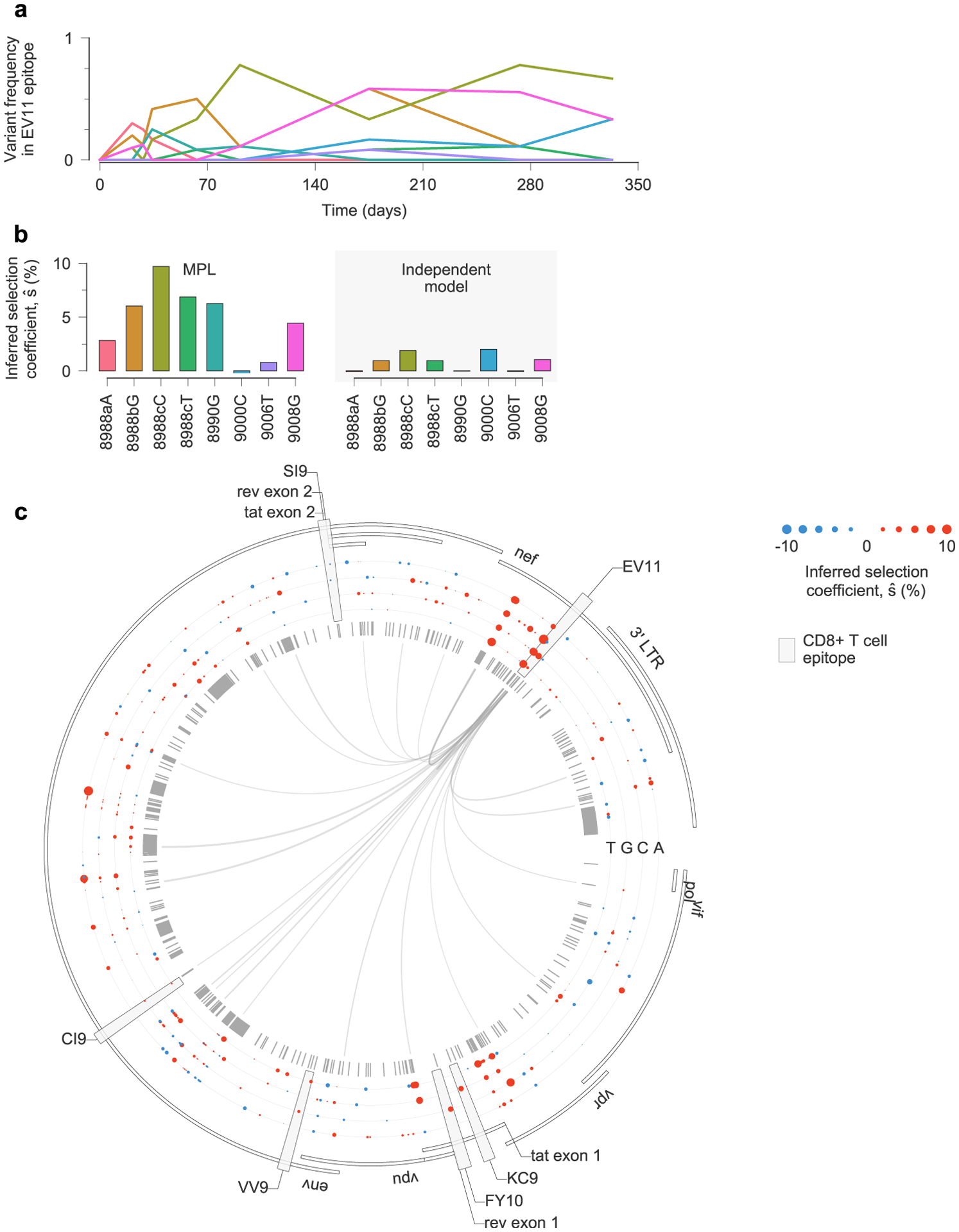
a, Multiple escape variants for the Nef epitope EV11, targeted by individual CH131, interfere with one another over the course of nearly one year. Here we have omitted the trajectories for transient variants with a deletion at sites 8988a-8988c, which are insertions with respect to the HXB2 reference sequence. b, MPL infers that all nonsynonymous EV11 escape variants are positively selected. Variants 9000C and 9006T are both synonymous, and are inferred to be nearly neutral by MPL. As in previous examples, inferences using only the trajectories of individual variants only infer substantial positive selection for variants that are polymorphic at the final time point, or where the transmitted/founder (TF) allele at the same site appears strongly selected against. In the latter case, positive selection is inferred because all selection coefficients are normalized such that the selection coefficient for the TF variant is zero. This is why the independent model infers 8988T to be beneficial despite its low frequency at the final time point. Note that the independent model also infers the synonymous mutation 9000C to be beneficial. c, Inferred selection in the HIV-1 3′ half-genome sequence for CH131. Inferred selection coefficients are plotted in tracks. Coefficients of TF nucleotides are normalized to zero. Tick marks denote polymorphic sites. Inner links, shown for sites connected to the EV11 epitope, have widths proportional to matrix elements of the inverse of the integrated covariance. Linked sites affect selection estimates within the epitope.
Extended Data Fig. 10 |. inferred selection coefficients across patients using different conventions for data processing.
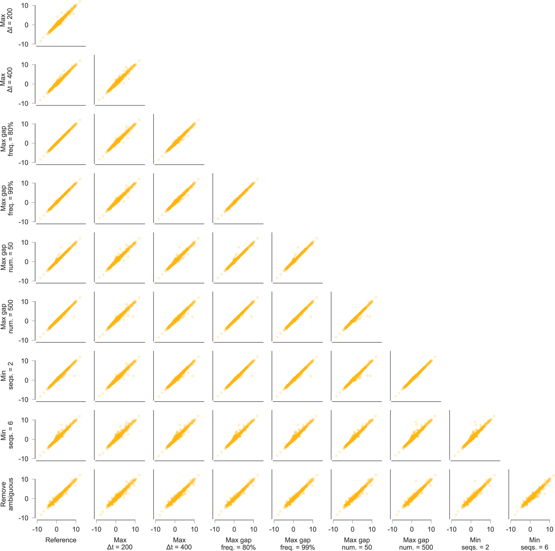
Inferred selection coefficients are highly similar following different choices for processing the sequence data. Pearson R2 values between inferred selection coefficients range from 0.97 to 1.00, with an average of 0.99. Data processing conventions. Reference: current data processing conventions. Max Δt = 200/400: remove time points that are more than 200/400 days beyond the last included time point (reference: 300 days). Max gap freq. = 80%/99%: remove sites where >80%/99% of observed variants are gaps (reference: 95%). Max gap num. = 50/500: remove sequences with >50/500 gaps in excess of subtype consensus (reference: 200). Min seqs. = 2/6: remove time points with <2/6 available sequences (reference: 4). Remove ambiguous: remove sequences that contain ambiguous nucleotides if any other nucleotide variation is observed at the same site. LTR, long terminal repeat.
Supplementary Material
Acknowledgements
We thank A.K. Chakraborty, C.J.R. Illingworth, B. Lee and J.G. Schraiber for helpful discussions and comments on the manuscript. The work of M.S.S., R.H.Y.L. and M.R.M. was supported by the Hong Kong Research Grants Council under grant number 16234716. M.S.S. and M.R.M. were also supported by the Hong Kong Research Grants Council under grant number 16201620, while R.H.Y.L. was also supported by Australia’s National Health and Medical Research Council under grant number APP1121643. The work of J.P.B. reported in this publication was supported by the National Institute of General Medical Sciences of the National Institutes of Health under award R35GM138233.
Footnotes
Online content
Any methods, additional references, Nature Research reporting summaries, source data, extended data, supplementary information, acknowledgements, peer review information; details of author contributions and competing interests; and statements of data and code availability are available at https://doi.org/10.1038/s41587-020-0737-3.
Data availability
Raw data used in our analysis is available in the GitHub repository located at https://github.com/bartonlab/paper-MPL-inference. Source data are provided with this paper.
Code availability
Code used in our analysis is available in the GitHub repository located at https://github.com/bartonlab/paper-MPL-inference. The repository also contains Jupyter notebooks that can be run to reproduce the results presented here. The source code is shared under GPL-3.0 license https://github.com/bartonlab/paper-MPL-inference/blob/master/LICENSE-GPL. An executable version is also provided on Code Ocean at https://codeocean.com/capsule/3400567/tree (ref. 30), distributed under the GPL-3.0 license https://opensource.org/licenses/gpl-license/.
Competing interests
The authors declare no competing interests.
Extended data is available for this paper at https://doi.org/10.1038/s41587-020-0737-3.
Supplementary information is available for this paper at https://doi.org/10.1038/s41587-020-0737-3.
References
- 1.Bignell GR et al. Signatures of mutation and selection in the cancer genome. Nature 463, 893–898 (2010). [DOI] [PMC free article] [PubMed] [Google Scholar]
- 2.Greaves M & Maley CC Clonal evolution in cancer. Nature 481, 306–313 (2012). [DOI] [PMC free article] [PubMed] [Google Scholar]
- 3.Burrell RA, McGranahan N, Bartek J & Swanton C The causes and consequences of genetic heterogeneity in cancer evolution. Nature 501, 338–345 (2013). [DOI] [PubMed] [Google Scholar]
- 4.Nik-Zainal S et al. The life history of 21 breast cancers. Cell 149, 994–1007 (2012). [DOI] [PMC free article] [PubMed] [Google Scholar]
- 5.Landau DA et al. Evolution and impact of subclonal mutations in chronic lymphocytic leukemia. Cell 152, 714–726 (2013). [DOI] [PMC free article] [PubMed] [Google Scholar]
- 6.Łuksza M et al. A neoantigen fitness model predicts tumour response to checkpoint blockade immunotherapy. Nature 551, 517–520 (2017). [DOI] [PMC free article] [PubMed] [Google Scholar]
- 7.McMichael AJ, Borrow P, Tomaras GD, Goonetilleke N & Haynes BF The immune response during acute HIV-1 infection: clues for vaccine development. Nat. Rev. Immunol 10, 11–23 (2010). [DOI] [PMC free article] [PubMed] [Google Scholar]
- 8.Allen TM et al. Selective escape from CD8+ T-cell responses represents a major driving force of human immunodeficiency virus type 1 (HIV-1) sequence diversity and reveals constraints on HIV-1 evolution. J. Virol 79, 13239–13249 (2005). [DOI] [PMC free article] [PubMed] [Google Scholar]
- 9.Zanini F et al. Population genomics of intrapatient HIV-1 evolution. eLife 4, e11282 (2015). [DOI] [PMC free article] [PubMed] [Google Scholar]
- 10.Strelkowa N & Lässig M Clonal interference in the evolution of influenza. Genetics 192, 671–682 (2012). [DOI] [PMC free article] [PubMed] [Google Scholar]
- 11.Łuksza M & Lässig M A predictive fitness model for influenza. Nature 507, 57–61 (2014). [DOI] [PubMed] [Google Scholar]
- 12.Muller HJ The relation of recombination to mutational advance. Mut. Res 1, 2–9 (1964). [DOI] [PubMed] [Google Scholar]
- 13.Smith JM & Haigh J The hitch-hiking effect of a favourable gene. Genet. Res 23, 23–35 (1974). [PubMed] [Google Scholar]
- 14.Hegreness M, Shoresh N, Hartl D & Kishony R An equivalence principle for the incorporation of favorable mutations in asexual populations. Science 311, 1615–1617 (2006). [DOI] [PubMed] [Google Scholar]
- 15.Lang GI et al. Pervasive genetic hitchhiking and clonal interference in forty evolving yeast populations. Nature 500, 571–574 (2013). [DOI] [PMC free article] [PubMed] [Google Scholar]
- 16.Tenaillon O et al. Tempo and mode of genome evolution in a 50,000-generation experiment. Nature 536, 165–170 (2016). [DOI] [PMC free article] [PubMed] [Google Scholar]
- 17.Levy SF et al. Quantitative evolutionary dynamics using high-resolution lineage tracking. Nature 519, 181–186 (2015). [DOI] [PMC free article] [PubMed] [Google Scholar]
- 18.Bollback JP, York TL & Nielsen R Estimation of 2Nes from temporal allele frequency data. Genetics 179, 497–502 (2008). [DOI] [PMC free article] [PubMed] [Google Scholar]
- 19.Malaspinas A-S, Malaspinas O, Evans SN & Slatkin M Estimating allele age and selection coefficient from time-serial data. Genetics 192, 599–607 (2012). [DOI] [PMC free article] [PubMed] [Google Scholar]
- 20.Mathieson I & McVean G Estimating selection coefficients in spatially structured populations from time series data of allele frequencies. Genetics 193, 973–984 (2013). [DOI] [PMC free article] [PubMed] [Google Scholar]
- 21.Feder AF, Kryazhimskiy S & Plotkin JB Identifying signatures of selection in genetic time series. Genetics 196, 509–522 (2014). [DOI] [PMC free article] [PubMed] [Google Scholar]
- 22.Lacerda M & Seoighe C Population genetics inference for longitudinally-sampled mutants under strong selection. Genetics 198, 1237–1250 (2014). [DOI] [PMC free article] [PubMed] [Google Scholar]
- 23.Foll M, Shim H & Jensen JD WFABC: a Wright–Fisher ABC–based approach for inferring effective population sizes and selection coefficients from time-sampled data. Mol. Ecol. Resour 15, 87–98 (2015). [DOI] [PubMed] [Google Scholar]
- 24.Ferrer-Admetlla A, Leuenberger C, Jensen JD & Wegmann D An approximate Markov model for the Wright–Fisher diffusion and its application to time series data. Genetics 203, 831–846 (2016). [DOI] [PMC free article] [PubMed] [Google Scholar]
- 25.Taus T, Futschik A & Schlötterer C Quantifying selection with Pool-Seq time series data. Mol. Biol. Evol 34, 3023–3034 (2017). [DOI] [PMC free article] [PubMed] [Google Scholar]
- 26.Illingworth CJR & Mustonen V Distinguishing driver and passenger mutations in an evolutionary history categorized by interference. Genetics 189, 989–1000 (2011). [DOI] [PMC free article] [PubMed] [Google Scholar]
- 27.Illingworth CJR, Fischer A & Mustonen V Identifying selection in the within-host evolution of influenza using viral sequence data. PLoS Comput. Biol 10, e1003755 (2014). [DOI] [PMC free article] [PubMed] [Google Scholar]
- 28.Terhorst J, Schlötterer C & Song YS Multi-locus analysis of genomic time series data from experimental evolution. PLoS Genet. 11, e1005069 (2015). [DOI] [PMC free article] [PubMed] [Google Scholar]
- 29.Sohail MS, Louie RHY, McKay MR & Barton JP, MPL resolves genetic linkage in fitness inference from complex evolutionary histories. Github https://github.com/bartonlab/paper-MPL-inference (2020). [DOI] [PMC free article] [PubMed] [Google Scholar]
- 30.Sohail MS, Louie RHY, McKay MR & Barton JP, MPL resolves genetic linkage in fitness inference from complex evolutionary histories. Code Ocean 10.24433/CO.1795728.v1 (2020). [DOI] [PMC free article] [PubMed] [Google Scholar]
- 31.Mustonen V & Lässig M Fitness flux and ubiquity of adaptive evolution. Proc. Natl Acad. Sci. USA 107, 4248–4253 (2010). [DOI] [PMC free article] [PubMed] [Google Scholar]
- 32.Illingworth CJR, Parts L, Schiffels S, Liti G & Mustonen V Quantifying selection acting on a complex trait using allele frequency time series data. Mol. Biol. Evol 29, 1187–1197 (2011). [DOI] [PMC free article] [PubMed] [Google Scholar]
- 33.Schraiber JG A path integral formulation of the Wright–Fisher process with genic selection. Theor. Popul. Biol 92, 30–35 (2014). [DOI] [PMC free article] [PubMed] [Google Scholar]
- 34.Ewens WJ Mathematical Population Genetics 1: Theoretical Introduction (Springer Science & Business Media, 2012). [Google Scholar]
- 35.Iranmehr A, Akbari A, Schlötterer C & Bafna V CLEAR: Composition of likelihoods for evolve and resequence experiments. Genetics 206, 1011–1023 (2017). [DOI] [PMC free article] [PubMed] [Google Scholar]
- 36.Liu MKP et al. Vertical T cell immunodominance and epitope entropy determine HIV-1 escape. J. Clin. Invest 123, 380–393 (2013). [DOI] [PMC free article] [PubMed] [Google Scholar]
- 37.Moore PL et al. Multiple pathways of escape from HIV broadly cross-neutralizing V2-dependent antibodies. J. Virol 87, 4882–4894 (2013). [DOI] [PMC free article] [PubMed] [Google Scholar]
- 38.Doria-Rose NA et al. Developmental pathway for potent V1V2-directed HIV-neutralizing antibodies. Nature 509, 55–62 (2014). [DOI] [PMC free article] [PubMed] [Google Scholar]
- 39.Liu Y et al. Selection on the human immunodeficiency virus type 1 proteome following primary infection. J. Virol 80, 9519–9529 (2006). [DOI] [PMC free article] [PubMed] [Google Scholar]
- 40.Neher RA & Leitner T Recombination rate and selection strength in HIV intra-patient evolution. PLoS Comput. Biol 6, e1000660 (2010). [DOI] [PMC free article] [PubMed] [Google Scholar]
- 41.Batorsky R et al. Estimate of effective recombination rate and average selection coefficient for HIV in chronic infection. Proc. Natl Acad. Sci. USA 108, 5661–5666 (2011). [DOI] [PMC free article] [PubMed] [Google Scholar]
- 42.Wang S et al. Manipulating the selection forces during affinity maturation to generate cross-reactive HIV antibodies. Cell 160, 785–797 (2015). [DOI] [PMC free article] [PubMed] [Google Scholar]
- 43.Liao H-X et al. Co-evolution of a broadly neutralizing HIV-1 antibody and founder virus. Nature 496, 469–476 (2013). [DOI] [PMC free article] [PubMed] [Google Scholar]
- 44.Ganusov VV et al. Fitness costs and diversity of the cytotoxic T lymphocyte (CTL) response determine the rate of CTL escape during acute and chronic phases of HIV Infection. J. Virol 85, 10518–10528 (2011). [DOI] [PMC free article] [PubMed] [Google Scholar]
- 45.Ganusov VV, Neher RA & Perelson AS Mathematical modeling of escape of HIV from cytotoxic T lymphocyte responses. J. Stat. Mech.: Theory Exp 2013, P01010 (2013). [DOI] [PMC free article] [PubMed] [Google Scholar]
- 46.Kessinger T, Perelson A & Neher R Inferring HIV escape rates from multi-locus genotype data. Front. Immunol 4, 252 (2013). [DOI] [PMC free article] [PubMed] [Google Scholar]
- 47.Pandit A & de Boer RJ Reliable reconstruction of HIV-1 whole genome haplotypes reveals clonal interference and genetic hitchhiking among immune escape variants. Retrovirology 11, 11–56 (2014). [DOI] [PMC free article] [PubMed] [Google Scholar]
- 48.Leviyang S & Ganusov VV Broad CTL response in early HIV infection drives multiple concurrent CTL escapes. PLoS Comput. Biol 11, e1004492 (2015). [DOI] [PMC free article] [PubMed] [Google Scholar]
- 49.Beerenwinkel N, Günthard HF, Roth V & Metzner KJ Challenges and opportunities in estimating viral genetic diversity from next-generation sequencing data. Front. Microbiol 3, 329 (2012). [DOI] [PMC free article] [PubMed] [Google Scholar]
- 50.Turajlic S, Sottoriva A, Graham T & Swanton C Resolving genetic heterogeneity in cancer. Nat. Rev. Genet 20, 404–416 (2019). [DOI] [PubMed] [Google Scholar]
- 51.Good BH, McDonald MJ, Barrick JE, Lenski RE & Desai MM The dynamics of molecular evolution over 60,000 generations. Nature 551, 45–50 (2017). [DOI] [PMC free article] [PubMed] [Google Scholar]
- 52.Kouyos RD, Althaus CL & Bonhoeffer S Stochastic or deterministic: what is the effective population size of HIV-1? Trends Microbiol. 14, 507–511 (2006). [DOI] [PubMed] [Google Scholar]
- 53.Cocco S, Feinauer C, Figliuzzi M, Monasson R & Weigt M Inverse statistical physics of protein sequences: a key issues review. Rep. Prog. Phys 81, 032601 (2018). [DOI] [PubMed] [Google Scholar]
- 54.Socolich M et al. Evolutionary information for specifying a protein fold. Nature 437, 512–518 (2005). [DOI] [PubMed] [Google Scholar]
- 55.Weigt M, White RA, Szurmant H, Hoch JA & Hwa T Identification of direct residue contacts in protein–protein interaction by message passing. Proc. Natl Acad. Sci. USA 106, 67–72 (2009). [DOI] [PMC free article] [PubMed] [Google Scholar]
- 56.Morcos F et al. Direct-coupling analysis of residue coevolution captures native contacts across many protein families. Proc. Natl Acad. Sci. USA 108, E1293–E1301 (2011). [DOI] [PMC free article] [PubMed] [Google Scholar]
- 57.Russ WP, Lowery DM, Mishra P, Yaffe MB & Ranganathan R Natural-like function in artificial WW domains. Nature 437, 579–583 (2005). [DOI] [PubMed] [Google Scholar]
- 58.Ferguson AL et al. Translating HIV sequences into quantitative fitness landscapes predicts viral vulnerabilities for rational immunogen design. Immunity 38, 606–617 (2013). [DOI] [PMC free article] [PubMed] [Google Scholar]
- 59.Mann JK et al. The fitness landscape of HIV-1 gag: advanced modeling approaches and validation of model predictions by in vitro testing. PLoS Comput. Biol 10, e1003776 (2014). [DOI] [PMC free article] [PubMed] [Google Scholar]
- 60.Figliuzzi M, Jacquier H, Schug A, Tenaillon O & Weigt M Coevolutionary landscape inference and the context-dependence of mutations in beta-lactamase TEM-1. Mol. Biol. Evol 33, 268–280 (2015). [DOI] [PMC free article] [PubMed] [Google Scholar]
- 61.Barton JP et al. Relative rate and location of intra-host HIV evolution to evade cellular immunity are predictable. Nat. Commun 7, 11660 (2016). [DOI] [PMC free article] [PubMed] [Google Scholar]
- 62.Hopf TA et al. Mutation effects predicted from sequence co-variation. Nat. Biotechnol 35, 128–135 (2017). [DOI] [PMC free article] [PubMed] [Google Scholar]
- 63.Louie RHY, Kaczorowski KJ, Barton JP, Chakraborty AK & McKay MR Fitness landscape of the human immunodeficiency virus envelope protein that is targeted by antibodies. Proc. Natl Acad. Sci. USA 115, E564–E573 (2018). [DOI] [PMC free article] [PubMed] [Google Scholar]
- 64.Quadeer AA, Louie RHY & Mckay MR Identifying immunologically-vulnerable regions of the HCV E2 glycoprotein and broadly neutralizing antibodies that target them. Nat. Commun 10, 2073 (2019). [DOI] [PMC free article] [PubMed] [Google Scholar]
- 65.Quadeer AA, Barton JP, Chakraborty AK & McKay MR Deconvolving mutational patterns of poliovirus outbreaks reveals its intrinsic fitness landscape. Nat. Commun 11, 377 (2020). [DOI] [PMC free article] [PubMed] [Google Scholar]
- 66.Kimura M Diffusion models in population genetics. J. Appl. Probab 1, 177–232 (1964). [Google Scholar]
- 67.Tataru P, Bataillon T & Hobolth A Inference under a Wright-Fisher model using an accurate beta approximation. Genetics 201, 1133–1141 (2015). [DOI] [PMC free article] [PubMed] [Google Scholar]
- 68.He Z, Beaumont M & Yu F Effects of the ordering of natural selection and population regulation mechanisms on Wright-Fisher models. G3: Genes, Genomes, Genetics 7, 2095–2106 (2017). [DOI] [PMC free article] [PubMed] [Google Scholar]
- 69.Tataru P, Simonsen M, Bataillon T & Hobolth A Statistical inference in the Wright-Fisher model using allele frequency data. Syst. Biol 66, e30–e46 (2017). [DOI] [PMC free article] [PubMed] [Google Scholar]
- 70.Risken H The Fokker–Planck Equation: Methods of Solution and Applications 2nd edn (Springer, 1989). [Google Scholar]
- 71.Gaschen B, Kuiken C, Korber B & Foley B Retrieval and on-the-fly alignment of sequence fragments from the HIV database. Bioinformatics 17, 415–418 (2001). [DOI] [PubMed] [Google Scholar]
- 72.Korber B et al. in Human Retroviruses and AIDS (eds Korber B et al.) 102–111 (Los Alamos National Laboratory, 1998).. [Google Scholar]
- 73.Zanini F, Puller V, Brodin J, Albert J & Neher RA In vivo mutation rates and the landscape of fitness costs of HIV-1. Virus Evol. 3, vex003 (2017). [DOI] [PMC free article] [PubMed] [Google Scholar]
Associated Data
This section collects any data citations, data availability statements, or supplementary materials included in this article.


