Deep learning for carotid plaque segmentation using a dilated U-Net architecture

Abstract

Carotid plaque segmentation in ultrasound longitudinal B-mode images using deep learning is presented in this work. We report on 101 severely stenotic carotid plaque patients. A standard U-Net is compared with a dilated U-Net architecture in which the dilated convolution layers were used in the bottleneck. Both a fully automatic and a semi-automatic approach with a bounding box was implemented. The performance degradation in plaque segmentation due to errors in the bounding box is quantified. We found that the bounding box significantly improved the performance of the networks with U-Net Dice coefficients of 0.48 for automatic and 0.83 for semi-automatic segmentation of plaque. Similar results were also obtained for the dilated U-Net with Dice coefficients of 0.55 for automatic and 0.84 for semi-automatic when compared to manual segmentations of the same plaque by an experienced sonographer. A five percent error in the bounding box in both dimensions reduced the Dice coefficient to 0.79 and 0.80 for U-Net and dilated U-Net respectively.

Introduction

Accurate segmentation of carotid plaques on B-mode images allows for quantification of useful biomechanical properties. Various elastography methods require plaque segmentation as the starting point^1–5, for accurate quantification of strain indices assessing plaque vulnerability. Carotid plaque presents on B-mode ultrasound images as either echogenic (bright), echolucent (dark), calcific with acoustic shadowing and heterogeneous with mixture of more than one plaque type⁶. This makes carotid plaque segmentation a challenging task and is typically performed manually by experienced sonographers.

Several research groups have implemented methods for carotid plaque segmentation. Destrempes et al. 2011⁷ developed a method where the user provided a manual segmentation of plaque in the first image of the video sequence, following which motion estimation and a Bayesian model was used to estimate plaque boundaries in the remaining frames of the video loop. McCormick et al. 2012¹ also developed a method where manual segmentation of plaque at end diastole frame was performed, with the segmented plaque region tracked over the rest of the cardiac cycle with displacement estimation made using a multi-level coarse to fine approach⁸ and Bayesian regularization⁹. The aim of this paper is to eliminate the need of the initial manual segmentation. Segmentation approaches described in references^1,7, are classified as manual segmentation, while a semi-automatic segmentation method is defined to be where a user only needs to provide minimal inputs such as a bounding box or seed points and the algorithm utilized provides the initial segmentation. A fully automatic method is defined to be one where no input from the user is needed other than selecting the B-mode image that needs to be segmented.

Recently deep neural networks have been used for automatic segmentation, especially those using convolutional Neural networks (CNN) in a U shaped structure or U-Net, have shown promising segmentation results in biomedical image segmentations¹⁰. The success of U-Net was due to the use of contracting or encoding layers followed by up-sampling or decoding layers that increase the resolution of the output. Moreover, with the use of skip connection the network could aggregate multi-scale information. Another CNN architecture that is used for segmentation and accomplishes the same effect are dilated convolution networks¹¹. The advantage with dilated networks are that there is no need for down and up-sampling and is suitable for dense prediction tasks such as segmentation.

Deep learning has been used for several ultrasound based image segmentation tasks^12–18. Use of three-dimensional (3D) data sets provide significant improvements when compared to 2D data sets^12,13,18. Qiu et al.¹³ developed a fully automatic segmentation method using CNN for 3D segmentation of the brain ventricle structure in embryonic mice. Their implementation consisted of a two-stage process where the first stage performed localization of the relevant structure within a bounding box, which was then supplied as an input to the second stage, which performed the segmentation. Leclerc et al.¹⁴ compared deep learning methods to traditional segmentation methods for 2D echocardiography segmentation and found that deep learning methods outperformed the latter. Moreover, they did not observe any significant additional improvements over U-Net when compared to more sophisticated networks with auxiliary loss, stacked hourglasses and dense skip connections¹⁴. Behboodi et al.¹⁵ demonstrated breast lesion segmentation using U-Net with limited annotated data using transfer learning and data augmentation.

Deep learning has also been used for ultrasound carotid plaque segmentation^16,17. Zhou et al.¹⁶ utilized U-Net to segment carotid plaques utilizing 3D ultrasound data sets on human subjects with >60% stenosis. They obtained a Dice coefficient of 0.9 with U-Net, which was an improvement over a previous approach using level sets with a Dice coefficient of 0.88. However, these results were obtained on fewer human subjects (n=13) and utilized 3D data sets in subjects without significant acoustic shadowing artifacts. Lekadir et al.¹⁷ used a CNN based classifier to distinguish between plaque composition characteristics such as lipid core, fibrous tissue and calcified tissue based on the echogenicity of these different components. Deep learning has also been utilized for segmentation and measurement of carotid intima-media thickness (CIMT), which is more amenable to these approaches due to the well-defined structure being identified^18–20.

In an online segmentation competition²¹ a U-Net combined with a dilated network was one of the winning solutions²². This method combined two popular networks for segmentation tasks which are the U-Net¹⁰ and dilated convolution network¹¹. We therefore adapted this approach for carotid plaque segmentation in our data sets. We also compared this dilated convolutional network with U-Net. A dilated convolution¹¹ is similar to a regular convolution where the kernel weights are convolved with image data. However, in dilated convolution the image data is strided. For example, dilation factor of 2 would mean the convolution will occur with every alternate image pixel and 3 would mean it occurs with every third pixel. In this paper we investigate two approaches for plaque segmentation, a fully automatic approach where the acquired image is directly passed on to the network and a semi-automatic approach where a sonographer provides a bounding box which is then used as input to the segmentation.

MATERIALS AND METHODS:

Human Patients and Data

We report on 101 in vivo patients who present with severe stenotic carotid plaques, clinically indicated for a carotid endarterectomy at University of Wisconsin-Madison. The study was approved by institutional IRB and the patients provided informed consent prior to any research scans. Radio frequency (RF) data from a Siemens S2000 system (Siemens Ultrasound, Mountain View, CA, USA) with an 18L6 transducer was obtained. Clinical B-mode data and color Doppler were obtained using a 9L4 transducer. Ultrasound data was acquired for three views of the carotid, namely the common carotid, carotid bifurcation and internal carotid on both left and right carotids for each patient. A total of 352 views with plaque were obtained. In each view, the sonographer manually segmented plaque at two to three end diastolic frames on B-mode image frames that were converted form RF data acquired. The sonographer also used clinical B-mode and color Doppler images for guiding the segmentation process. Ultrasound strain imaging²³ on parts of these data set has been reported in previous studies^2,24,25 that used manual segmentation that were then tracked over the entire cardiac cycle. This manual segmentation is now used as the ground truth for training and testing the networks.

Network and Training Specifications

The dilated U-Net used in this paper is presented in Fig. 1. In contrast to the traditional U-Net that uses four down-sampling and up-sampling stages each, this network has three stages. The bottleneck or the middle section has six dilated convolution layers where the traditional U-Net has three convolution layers. The dilated U-Net has 22 convolution layers and 4.5 million trainable parameters. The U-Net used for comparison in this paper has 24 convolution layers and 11 million trainable parameters.

Figure 1:

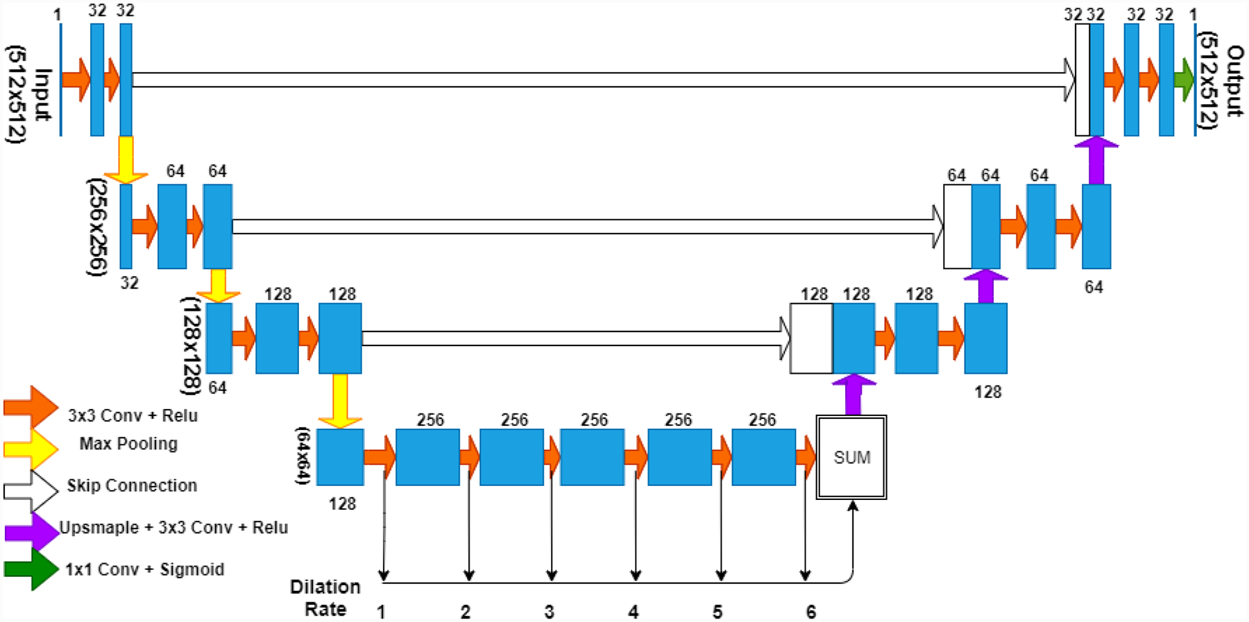
CNN model used in the paper, combines U-Net and dilated CNN. Three levels of max pooling and up sampling are used and 6 layers of dilated convolutions are used in the bottleneck with dilation rates from 1 through 6.

The 352 plaque views were divided into training, validation and testing sets, with 90% of the data used for training and validation and 10% for testing. Within the training and validation data sets, the split used was 95-5. Since each patient or view had multiple, end diastolic frame segmentations a total of 862 frames were available. The original B-mode images for a typical 4 cm depth acquisition were of size 455 (width) × 691(depth) pixels. The frames were resampled to size of 512×512 pixels. The networks were trained using back propagation and the ‘rmsprop’ algorithm²⁶. Dice loss and binary cross entropy (BCE) were separately used as loss functions for training. The networks performed slightly better with BCE and hence it was chosen as the loss function used for this paper. Dice coefficient, Dice loss and BCE loss are defined by the following formulae:

$$\mathit{\text{Dice coefficent}}=\frac{2\left|y\cap p\right|}{y+p}$$

$$\mathit{\text{Dice loss}}=1-\text{ Dice coefficent}$$

$$\mathit{\text{BCE loss}}=-\left(\mathit{\text{ylog}}\left(p\right)+\left(1-y\right)\mathit{\text{log}}\left(1-p\right)\right)$$

Here y is the ground truth and p is the prediction made by the network. For calculating the Dice coefficient, thresholding is performed such that values greater than 0.5 are made equal to 1 and lower than 0.5 are made equal to 0. This is not required for the BCE function and this function is directly available in the keras library which is implemented to handle any possible corner cases.

The initial learning rate was 10E-4. The learning rate was reduced by a factor of 0.2 every time the performance of the networks did not improve for three consecutive epochs on the validation set. The networks were run for up to 35 epochs. The training was stopped if the network performance did not improve for eight consecutive epochs. Online data augmentation was provided by random horizontal, vertical and horizontal-vertical flips. A NVIDIA Tesla K40c GPU (NVIDIA Corporation, Santa Clara, CA, USA) with an Intel(R) Xeon(R) CPU E5-2640 v4 (Intel Corporation, Santa Clara, CA, USA) was used to run the networks. The dilated U-Net took about 200 second per epoch and U-Net took about 218 seconds per epoch.

For the semi-automatic bounding box approach, an example is illustrated in Fig. 2. The sonographer is expected to provide a rectangular region i.e. the red box bounding the plaque and the algorithm adds an additional 12.5% buffer on all sides of the red box. This was done with the intent of having 75% plaque and 25% background along the axes of the input. It should also be noted that this is done for each plaque region. Thus for Fig. 2 which has three separate plaque regions the sonographer will perform the process three times. The region within the bounding box was resampled to a size of 256×256 pixels, smaller than the input image size of 512×512 pixels accounting for the smaller size of the plaque regions when compared to the entire B-mode frame. Thus, semi-automatic networks had input and output image size of 256×256 pixels.

Figure 2:

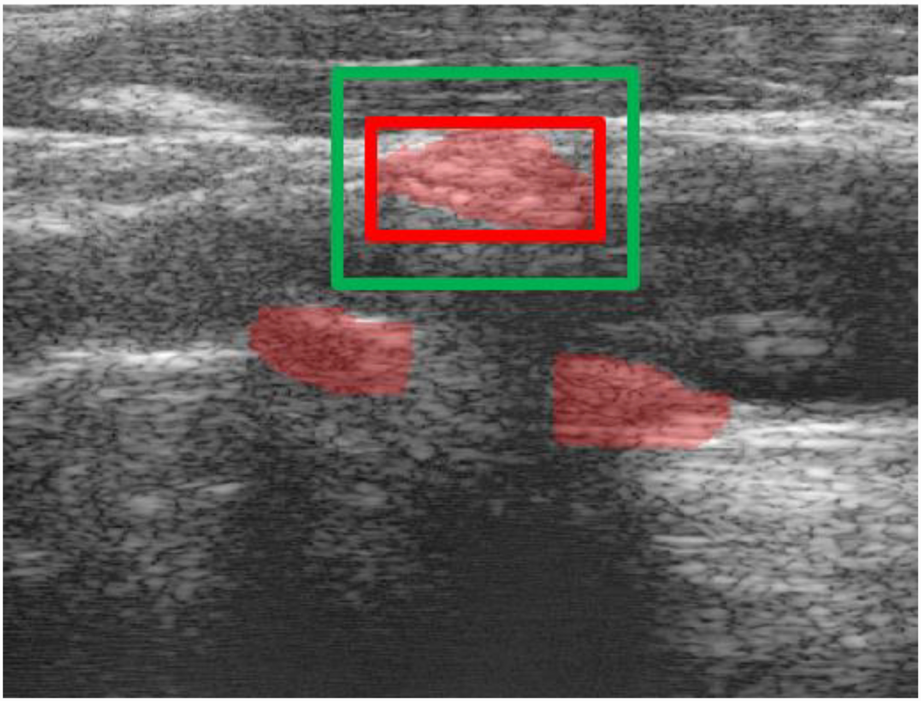
The sonographer will provide a bounding box (red) the system will construct the corresponding segmentation view (green) with 12.5% buffer on all sides.

The bounding box was automatically derived from the ground truth segmentation. However, to account for offset and overall size variations that a sonographer could make while providing the bounding boxes. The dimensions of the boxes derived from the ground truth were randomly varied from between 4% to −4% and the boxes were offset between 6.25% to −6.25% in training which is half of the buffer region in both directions. Along with making the networks more robust for practical use this also provides additional data augmentation.

The flow chart for our segmentation method is presented in Fig. 3. The B-mode image is first resampled based on the bounding box. The resampled B-mode image is then provided as an input to the network, which then provides the segmented region as the output. The output is then resampled back to the original view, i.e. same as the initial B-mode frame dimensions. The training for the semi-automatic method was performed independent of the automatic method.

Figure 3:

Flow chart of proposed segmentation method

All code used in this work along with trained model weights is available at https://github.com/Nirvedh/DeepPlaque.

Results

The performance of the automatic setup for segmentation is presented in Fig. 4. We consider a Dice coefficient of greater than or equal to 0.75 (which is set as our threshold) as a success and those with lower Dice coefficient values to be failures. Figure 4 shows that around 12 of the 121 test cases were successful for both the U-Net and dilated U-Net. We can also observe that the dilated U-Net performed generally better for the low Dice coefficient cases.

Figure 4:

Dice coefficient for test cases using U-Net and dilated U-Net with a usable threshold of 0.75

The performance of the semi-automatic setup is presented in Fig. 5. We use the same Dice coefficient threshold of greater than or equal to 0.75 as a successful segmentation. Figure 5 shows that with semi-automated segmentation 109 of the 121 test cases were successful using U-Net and 114 for the dilated U-Net. The performance of both networks was similar except for the lower performing cases where dilated U-Net provided better segmentation results. This is similar to the performance obtained with the automatic segmentation setup.

Figure 5:

Dice coefficient for test cases using semi automatic U-Net and dilated U-Net with a usable threshold of 0.75

The overall mean Dice coefficient along with standard deviation for both networks and both setups are presented in Table 1. The mean DC for dilated U-Net was 0.55 for the automatic setup while it was 0.48 for the U-Net. The difference was less significant with 0.84 and 0.83 respectively for the semi-automatic segmentation setup.

Table 1:

Dice Performance Statistics

Network Type	Dice mean	Dice standard deviation
U-Net	0.48	0.24
Dilated U-Net	0.55	0.19
Semi U-Net	0.83	0.05
Semi dilated U-Net	0.84	0.05

For the semi-automatic method, the Hausdorff error (HE) which is the maximum distance between the manual segmentation and the network segmentation and the Mean error (ME) which is the average distance between the two segmentations were quantified in Table 2. The dilated U-Net had slightly lower distances and hence slightly better overall performance.

Table 2:

Hausdorff error (HE) and Mean error (ME) for the semi automatic methods

Network Type	Average HE (mm)	Average ME (mm)
U-Net	1.71	0.38
Dilated U-Net	1.60	0.35

It is also of interest to ascertain how the performance of the network would vary with errors in the bounding boxes. This is quantified in Table 3 for the U-Net. The zero error average Dice coefficient value of 0.83 is 0.79 when an error of 5% is introduced along both axes. For the dilated U-Net these results are presented in Table 4. The average Dice coefficients are 0.84 and 0.80 respectively for the two cases.

Table 3:

offset sensitivity of U-Net dice coefficient

Offset in x-direction Offset in y-direction	−5%	0%	5%
−5%	0.79	0.80	0.81
0%	0.80	0.83	0.81
5%	0.79	0.81	0.79

Table 4:

offset sensitivity of dilated U-Net dice coefficient

Offset in x-direction Offset in y-direction	−5%	0%	5%
−5%	0.80	0.82	0.80
0%	0.81	0.84	0.81
5%	0.80	0.82	0.80

Discussion

There are two key observations from this paper. First, the performance of both U-Net CNN improved significantly after the bounding box was incorporated for semi-automated segmentation. Second, the dilated U-Net provides a better performance for the more difficult and complex plaque segmentations. The reason for improvement with the bounding box is the wide range of plaque shapes and echogenicity variations in the B-mode images and the corresponding background that the network had to segment. This is visualized by observing Fig. 6 and Fig. 7 that show two images of the carotid artery with plaque. Note that it is difficult for an untrained observer to even roughly identify plaque regions making plaque segmentation a challenging problem to solve. For better visualization of the segmentations we present the contours of the segmented regions. Fig. 6(b) and Fig. 7(b) with bounding box provide better segmentation compared to Fig. 6(a) and Fig. 7(a) without the bounding box. In Fig. 6, all four networks were able to correctly identify the location of plaque. However, the semi-automatic networks did provide superior segmentation due to their limited scope. In Fig. 7(a) both networks have Dice coefficients of 0. This low performance by the automatic approach was seen when faced with an acquisition that was unique compared to anything observed in the training set. For instance, in Fig. 7(a) there is an artery with significant curvature which is not extremely common in most acquisitions.

Figure 6:

Plaque segmentation example 1 with red contour as ground truth: (a) U-Net (yellow) (DC=0.77) and Dilated U-Net (green) (DC=0.88), (b)Semi automatic (yellow) U-Net (DC=0.83) and Semi automatic dilated U-Net (DC=0.87)

Figure 7:

Plaque segmentation example 2 with red contour as ground truth: (a) U-Net (yellow) (DC=0) and Dilated U-Net (no segmentation provided by the network) (DC=0), and a zoomed in view with (b)Semi automatic U-Net (yellow) (DC=0.92) and Semi automatic dilated U-Net (green) (DC=0.92)

Figures 6(a) present with Dice coefficients of 0.77 and 0.88 for U-Net and dilated U-Net respectively, here the U-Net segmentation is not as good as the one obtained with the dilated U-Net. The dilated U-Net is able to identify features better in lower performing situations with more complex plaque. At the same time in situations where the networks could provide high quality segmentations such as Fig. 6(b) with Dice coefficients of 0.83, and 0.87 and also 7(b) with Dice coefficients of 0.92 in both cases we observe that the two networks do not perform significantly different. This is similar to the observation made by Leclerc et al.¹⁴ that reported no significant difference between U-Net and more sophisticated networks.

The Dice coefficient threshold of 0.75 was used with the intention of quantifying success of the network since from visual inspection if the Dice co-efficient values were below 0.75, the value of that segmentation to the sonographer may be questionable. However, this was an arbitrary threshold which was used to make performance comparisons between the networks

Zhou et al.¹⁶ used U-Net for segmentation of 3D plaques in transverse view. They provided the network with data that were segmented with an initial contour of media-adventitia and lumen-media boundaries, following which the network was used to segment the plaque. They obtained a Dice coefficient of 0.91 while our network provided a Dice coefficient of 0.84 which is lower. Some reasons for this may be use of 3D versus 2D datasets, initial contours provided, and the lower image quality of B-mode images generated from research RF data in this work compared to clinical B-mode images used in Zhou et al.¹⁶. However, for the purpose of quantitative ultrasound imaging applications, it is necessary to use RF data. Additionally, while our bounding box reduced the field of view where the network had to segment the plaque and hence resulted in performance improvement, our network can autonomously identify adventitia and lumen boundaries while the results in Zhou et al.¹⁶ are based on pre segmented boundaries.

It is of interest to understand the behaviour of the semi-automatic networks when the bounding box only includes part of the plaque region. To examine this in Fig. 8, we provide the dilated network with a bounding box that only contains part of the plaque shown in Fig. 6. It is observed that the network segments the part of the plaque but does not segment close to the bounding boxes edges as typically that part did not contain plaque during training. It is also able to segment the carotid wall where plaque was not present.

Figure 8:

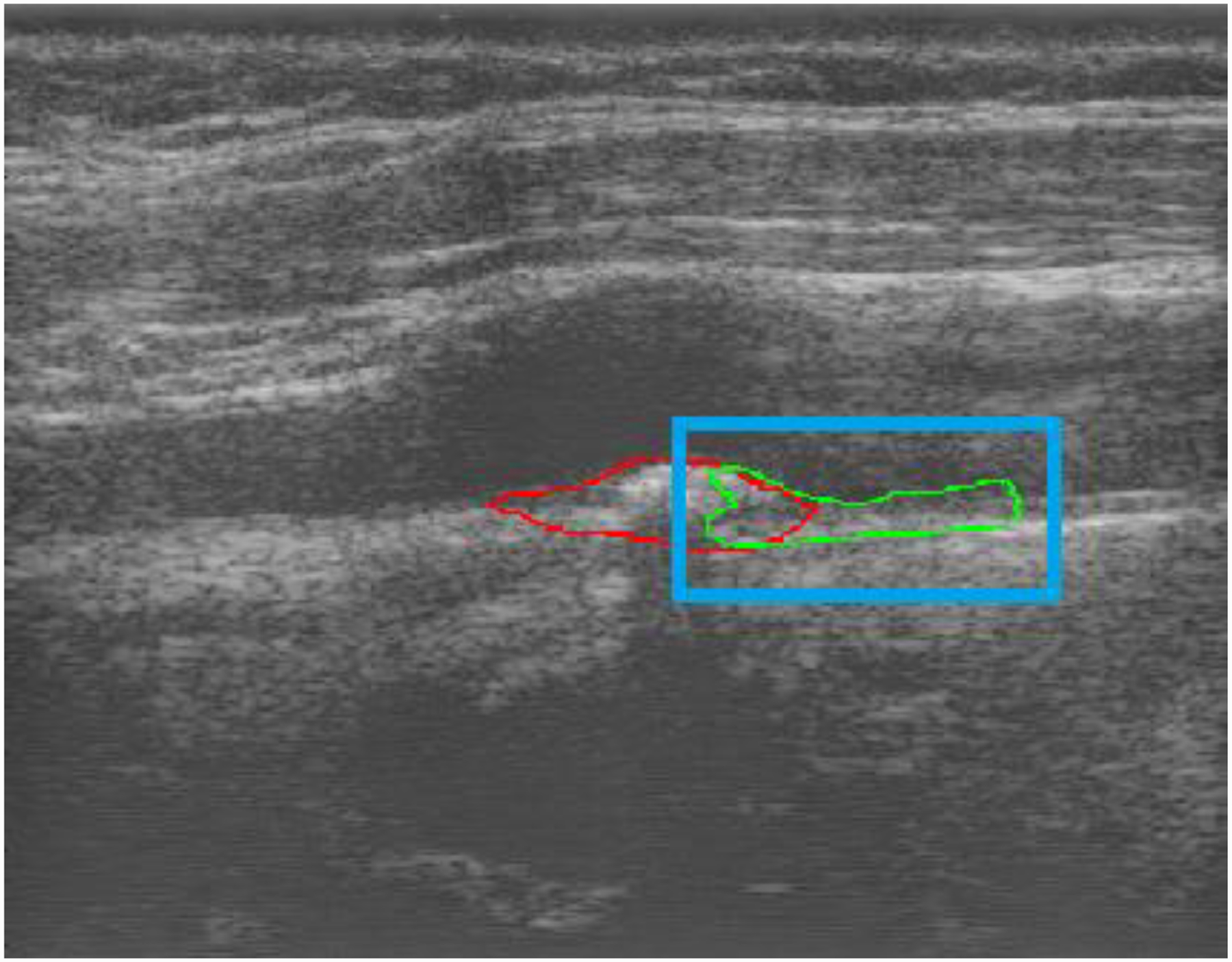
Performance of dilated U-Net model with bounding box including only part of a plaque, red is ground truth and green is network segmentation and blue is the bounding box provided. For interpretation of the references to colours in this figure legend, refer to the online version of this article.

It is also of interest to observe the performance of network when provided with a healthy volunteer with no plaque. Figure 9 shows the segmentation obtained on common carotid walls of a 24-year-old healthy female volunteer. The ground truth red segmentation on the carotid walls with adventitia layer included was provided by an experienced sonographer. A bounding box was set around each wall segment based on the sonographer segmentation to examine the network performance. It is observed that the network is able to easily segment the carotid walls when plaque is not present in healthy volunteers. Several other studies have previously provided carotid wall segmentation such as Loizou et. al.²⁷ with a snakes based segmentation method and also with neural network approaches by Menchón-Lara et al.²⁸ and Biswas et al.²⁹. Thus the same network can provide segmentations for arterial walls and plaques

Figure 9:

Performance of dilated U-Net model for a healthy subject with no plaque, red is ground truth and green is network segmentation.

The choice of 10E-4 as initial learning rate was made as it was found to be large enough to enable the network to get trained to estimate the optimal parameters. However, it was important to reduce the learning rate appropriately when the performance of the network did not improve, so that the network can be fine-tuned for optimal performance. The choice of training up to 35 epochs and stopping thereafter if no improvements were seen after this point, since we did not want to over-fit our training set. To demonstrate this behaviour of the network, Fig. 10 presents three runs of both the U-net and dilated U-net for the training set in Fig. 10(a) and 10(b). The validation set that was used to tune the training process is shown in Fig. 10(c) and 10(d), while the testing set that the network was completely blinded to is shown in Fig. 10(e) and 10(f) for U-net and dilated U-net respectively. In the first run shown by the blue marker we let the networks run for 50 epochs. In the next two runs we used 35 epochs along with our stopping criteria of non-improvement for 8 epochs in the validation set. We observe that across all sets the performance is similar in the three runs and hence our stopping criteria and number of epochs are sufficient. We also observe initial volatile behaviour attributed to high initial learning rate in all the runs which converges as the learning rate is reduced on our criteria of non-improvement for 3 epochs. The three sets have similar performance which indicates that we did not have an over-fitting problem in our network and hence the number of layers chosen in the network was appropriate for this dataset.

Figure 10:

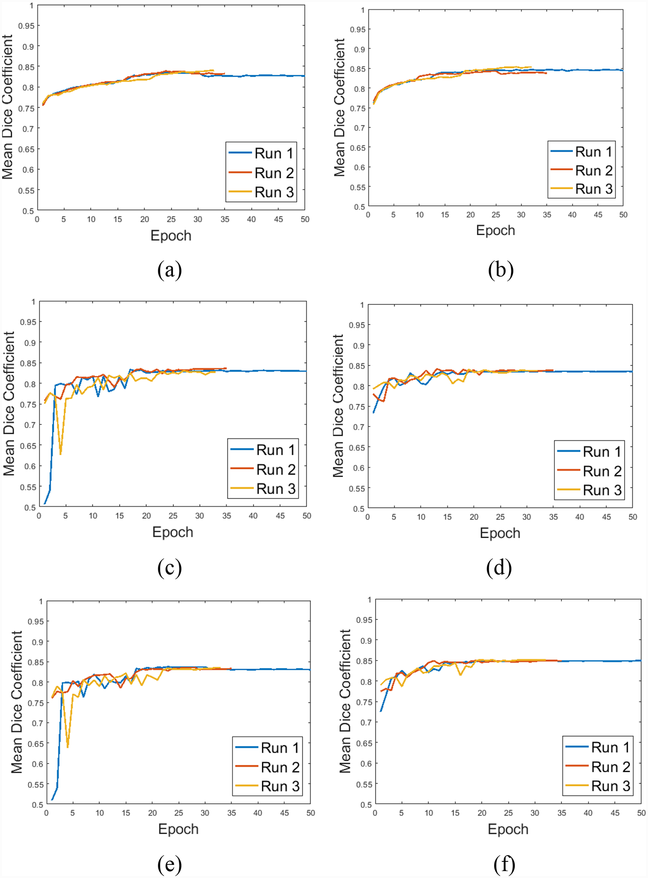
Training behavior over three independent runs, (a) and (b) in training, (c) and (d) in validation, (e) and (f) in the testing set for U-Net and dilated U-Net respectively

An interesting part of this dataset was the presence of two to three cardiac cycles of RF data for each acquisition. As previously mentioned the sonographer had segmented up to three end diastole frames in each acquisition. Our initial attempt was to treat each segmentation as an individual dataset and randomly distribute them in our training, validation and testing set. However, this caused overfitting because if frames of the same view existed across the three sets then the network could easily learn the segmentation for those plaques without actually learning the features required to segment. Hence, we had to split the data at the acquisition level instead of the frame level. Thus the multiple frames may provide modest additional data augmentation but cannot be used as additional data. Another aspect to consider in future work with the temporal dimension of data was to provide multiple consecutive data frames to the network so that based on pixel movement the network could separate blood flow from tissue and use that information to better segment plaques. In fact, as previously mentioned the sonographer does use clinically acquired color Doppler imaging to guide the manual segmentation process and hence this would be a natural extension for the network to do as well.

The sensitivity analysis also demonstrates that while the performance does degrade if the bounding boxes are not accurately placed, the degradation is within expected limits. This was possible because similar errors were also incorporated in training which ensured that the network could handle these errors. Qiu et al.¹³ and Amiri et al.³⁰ utilized another CNN to identify the correct bounding box prior to performing the segmentation. This would be challenging in our diverse dataset as we observe from Fig. 7(a) where the automatic U-Net could not even detect the correct location of the plaque in the B-mode image.

Conclusion

Severely stenotic carotid plaques in carotid endarterectomy patients with stenosis >70%, were segmented using U-Net style convolution neural networks. Sonographer input via a bounding box on plaque was required to achieve acceptable segmentation performance on these carotid B-mode images on patients with significant plaque and associated shadowing artifacts. Presence of acoustic shadowing has a significant impact on the performance of the segmentation algorithms and represent cases encountered under imaging conditions for carotid endarterectomy patients. A dilated U-Net option that provides improved performance in challenging segmentation situations when compared to U-Net was also presented.

References

- 1.McCormick M, Varghese T, Wang X, Mitchell CC, Kliewer M, Dempsey RJ, Methods for robust in vivo strain estimation in the carotid artery, Physics in Medicine and Biology 57, 7329 (2012). [DOI] [PMC free article] [PubMed] [Google Scholar]
- 2.Meshram NH, Varghese T, Mitchell CC, Jackson DC, Wilbrand SM, Hermann BP, Dempsey RJ, Quantification of carotid artery plaque stability with multiple region of interest based ultrasound strain indices and relationship with cognition, Physics in Medicine and Biology 62, 6341–6360 (2017). [DOI] [PMC free article] [PubMed] [Google Scholar]
- 3.de Korte CL, Fekkes S, Nederveen AJ, Manniesing R, Hansen HRH, Mechanical characterization of carotid arteries and atherosclerotic plaques, IEEE transactions on ultrasonics, ferroelectrics, and frequency control 63, 1613–1623 (2016). [DOI] [PubMed] [Google Scholar]
- 4.Apostolakis IZ, Karageorgos GM, Nauleau P, Nandlall SD, Konofagou EE, Adaptive Pulse Wave Imaging: automated spatial vessel wall inhomogeneity detection in phantoms and in-vivo, IEEE Transactions on Medical Imaging (2019). [DOI] [PMC free article] [PubMed] [Google Scholar]
- 5.Nayak R, Huntzicker S, Ohayon J, Carson N, Dogra V, Schifitto G, Doyley MM, Principal strain vascular elastography: Simulation and preliminary clinical evaluation, Ultrasound in Medicine and Biology 43, 682–699 (2017). [DOI] [PMC free article] [PubMed] [Google Scholar]
- 6.Geroulakos G, Ramaswami G, Nicolaides A, James K, Labropoulos N, Belcaro G, Holloway M, Characterization of symptomatic and asymptomatic carotid plaques using high‐resolution real‐time ultrasonography, British Journal of Surgery 80, 1274–1277 (1993). [DOI] [PubMed] [Google Scholar]
- 7.Destrempes F, Meunier J, Giroux M-F, Soulez G, Cloutier G, Segmentation of plaques in sequences of ultrasonic B-mode images of carotid arteries based on motion estimation and a Bayesian model, IEEE Transactions on Biomedical Engineering 58, 2202–2211 (2011). [DOI] [PubMed] [Google Scholar]
- 8.Shi H, Varghese T, Two-dimensional multi-level strain estimation for discontinuous tissue, Physics in Medicine and Biology 52, 389 (2007). [DOI] [PubMed] [Google Scholar]
- 9.McCormick M, Rubert N, Varghese T, Bayesian regularization applied to ultrasound strain imaging, IEEE Transactions on Biomedical Engineering 58, 1612–1620 (2011). [DOI] [PMC free article] [PubMed] [Google Scholar]
- 10.Ronneberger O, Fischer P, Brox T, U-net: Convolutional networks for biomedical image segmentation, in International Conference on Medical image computing and computer-assisted intervention, pp. 234–241 (2015). [Google Scholar]
- 11.Yu F, Koltun V, Multi-scale context aggregation by dilated convolutions, arXiv preprint arXiv:1511.07122 (2015). [Google Scholar]
- 12.Orlando N, Gillies DJ, Gyacskov I, Romagnoli C, D’Souza D, Fenster A, Automatic prostate segmentation using deep learning on clinically diverse 3D transrectal ultrasound images, Med Phys Epub Mar 12, (2020). [DOI] [PubMed] [Google Scholar]
- 13.Qiu Z, Langerman J, Nair N, Aristizabal O, Mamou J, Turnbull DH, Ketterling J, Wang Y, Deep Bv: A Fully Automated System for Brain Ventricle Localization and Segmentation In 3D Ultrasound Images of Embryonic Mice, in 2018 IEEE Signal Processing in Medicine and Biology Symposium (SPMB), pp. 1–6 (2018). [DOI] [PMC free article] [PubMed] [Google Scholar]
- 14.Leclerc S, Smistad E, Pedrosa J, Østvik A, Cervenansky F, Espinosa F, Espeland T, Berg EAR, Jodoin P-M, Grenier T, Deep learning for segmentation using an open large-scale dataset in 2d echocardiography, IEEE Transactions on Medical Imaging (2019). [DOI] [PubMed] [Google Scholar]
- 15.Behboodi B, Amiri M, Brooks R, Rivaz H, Breast lesion segmentation in ultrasound images with limited annotated data, arXiv preprint arXiv:2001.07322 (2020). [Google Scholar]
- 16.Zhou R, Ma W, Fenster A, Ding M, U-Net based automatic carotid plaque segmentation from 3D ultrasound images, in Medical Imaging 2019: Computer-Aided Diagnosis, pp. 109504F (2019). [Google Scholar]
- 17.Lekadir K, Galimzianova A, Betriu À, del Mar Vila M, Igual L, Rubin DL, Fernández E, Radeva P, Napel S, A convolutional neural network for automatic characterization of plaque composition in carotid ultrasound, IEEE journal of biomedical and health informatics 21, 48–55 (2016). [DOI] [PMC free article] [PubMed] [Google Scholar]
- 18.Zhou R, Fenster A, Xia Y, Spence JD, Ding M, Deep learning-based carotid media-adventitia and lumen-intima boundary segmentation from three-dimensional ultrasound images, Med Phys 46, 3180–3193 (2019). [DOI] [PMC free article] [PubMed] [Google Scholar]
- 19.Vila MDM, Remeseiro B, Grau M, Elosua R, Betriu À, Fernandez-Giraldez E, Igual L, Semantic segmentation with DenseNets for carotid artery ultrasound plaque segmentation and CIMT estimation, Artif Intell Med 103, 101784 (2020). [DOI] [PubMed] [Google Scholar]
- 20.Biswas M, Kuppili V, Saba L, Edla DR, Suri HS, Sharma A, Cuadrado-Godia E, Laird JR, Nicolaides A, Suri JS, Deep learning fully convolution network for lumen characterization in diabetic patients using carotid ultrasound: a tool for stroke risk, Med Biol Eng Comput 57, 543–564 (2019). [DOI] [PubMed] [Google Scholar]
- 21.Kaggle, Carvana Image Masking Challenge, (2017).
- 22.Iyakaap, Kaggle-Carvana-3rd-Place-Solution, (2017).
- 23.Ophir J, Cespedes I, Ponnekanti H, Yazdi Y, Li X, Elastography: a quantitative method for imaging the elasticity of biological tissues, Ultrasonic Imaging 13, 111–134 (1991). [DOI] [PubMed] [Google Scholar]
- 24.Meshram NH, Mitchell CC, Wilbrand SM, Dempsey RJ, Varghese T, In vivo carotid strain imaging using principal strains in longitudinal view, Biomedical Physics & Engineering Express (2019). [DOI] [PMC free article] [PubMed] [Google Scholar]
- 25.Dempsey RJ, Varghese T, Jackson DC, Wang X, Meshram NH, Mitchell CC, Hermann BP, Johnson SC, Berman SE, Wilbrand SM, Carotid atherosclerotic plaque instability and cognition determined by ultrasound-measured plaque strain in asymptomatic patients with significant stenosis, Journal of Neurosurgery 128, 111–119 (2018). [DOI] [PMC free article] [PubMed] [Google Scholar]
- 26.Tieleman T, Hinton G, Lecture 6.5-rmsprop: Divide the gradient by a running average of its recent magnitude, COURSERA: Neural networks for machine learning 4, 26–31 (2012). [Google Scholar]
- 27.Loizou CP, Pattichis CS, Pantziaris M, Tyllis T, Nicolaides A, Snakes based segmentation of the common carotid artery intima media, Medical and Biological Engineering and Computing 45, 35–49 (2007). [DOI] [PubMed] [Google Scholar]
- 28.Menchón-Lara R-M, Sancho-Gómez J-L, Fully automatic segmentation of ultrasound common carotid artery images based on machine learning, Neurocomputing 151, 161–167 (2015). [Google Scholar]
- 29.Biswas M, Kuppili V, Araki T, Edla DR, Godia EC, Saba L, Suri HS, Omerzu T, Laird JR, Khanna NN, Deep learning strategy for accurate carotid intima-media thickness measurement: an ultrasound study on Japanese diabetic cohort, Computers in Biology and Medicine 98, 100–117 (2018). [DOI] [PubMed] [Google Scholar]
- 30.Amiri M, Brooks R, Behboodi B, Rivaz H, Two-stage ultrasound image segmentation using U-Net and test time augmentation, International Journal of Computer Assisted Radiology and Surgery (2020). [DOI] [PubMed] [Google Scholar]