Inference of population genetic parameters from an irregular time series of seasonal influenza virus sequences

Abstract

Basic summary statistics that quantify the population genetic structure of influenza virus are important for understanding and inferring the evolutionary and epidemiological processes. However, the sampling dates of global virus sequences in the last several decades are scattered nonuniformly throughout the calendar. Such temporal structure of samples and the small effective size of viral population hampers the use of conventional methods to calculate summary statistics. Here, we define statistics that overcome this problem by correcting for the sampling-time difference in quantifying a pairwise sequence difference. A simple linear regression method jointly estimates the mutation rate and the level of sequence polymorphism, thus providing an estimate of the effective population size. It also leads to the definition of Wright’s F_ST for arbitrary time-series data. Furthermore, as an alternative to Tajima’s D statistic or the site-frequency spectrum, a mismatch distribution corrected for sampling-time differences can be obtained and compared between actual and simulated data. Application of these methods to seasonal influenza A/H3N2 viruses sampled between 1980 and 2017 and sequences simulated under the model of recurrent positive selection with metapopulation dynamics allowed us to estimate the synonymous mutation rate and find parameter values for selection and demographic structure that fit the observation. We found that the mutation rates of HA and PB1 segments before 2007 were particularly high and that including recurrent positive selection in our model was essential for the genealogical structure of the HA segment. Methods developed here can be generally applied to population genetic inferences using serially sampled genetic data.

Introduction

Among the rapidly accumulating genetic information for evolutionary biological studies, temporal series of nucleotide sequences in a population are particularly valuable. While most population genetic studies indirectly infer evolutionary processes in the past from sequence diversity and polymorphism observed in the present, more direct inferences are possible if sampled sequences cover a period over which the evolutionary changes of interest unfold. In particular, the analysis of nucleotide sequences continuously sampled for many years from experimentally evolving organisms in laboratories (Schlötterer et al. 2015; Good et al. 2017; Van Den Bergh et al. 2018), from pathogens under surveillance by public health organizations (Holmes et al. 2016; FDA 2020), and from fossilized ancient individuals (Slatkin and Racimo 2016; https://oagr.org/) can reveal their rapid evolutionary changes directly. Serially sampled sequences allow the estimation of important evolutionary genetic parameters that is not possible with data obtained at a single time point. For example, various methods were proposed to estimate the strength of natural selection and effective population size (N_e) from allele frequency trajectories (Bollback et al. 2008; Steinrücken et al. 2014; Ferrer-Admetlla et al. 2016; Schraiber et al. 2016; Zinger et al. 2019). These studies assumed that nucleotide sequences are obtained at regular time intervals, with multiple sequences at a single time point, so that there is a discrete series of allele frequencies. However, as we explain below, a difficulty arises in determining allele frequencies from nucleotide sequences sampled without such a deliberate scheme to obtain regular time series. Accordingly, many summary statistics that are conventionally used in population genetic inferences may not be utilized because they were primarily developed for contemporaneous genetic data (Vitti et al. 2013). This current study develops evolutionary inferences that overcome such problems associated with irregular time-series genetic data, specifically as a solution to inferring complex evolutionary dynamics of seasonal influenza virus H3N2.

Being a major infectious disease agent in humans, the influenza virus has been heavily investigated for several decades, leading to large databases of publicly available genomic sequences (Shu and Mccauley, 2017 and the NCBI Influenza Virus Resource). Many studies demonstrated that influenza virus causing seasonal epidemics in humans, particularly subtype A/H3N2, is under strong selective pressure to evade the host immune response by altering the antigenic structure of surface proteins, hemagglutinin (HA) and neuraminidase (NA) (Nelson and Holmes 2007; Bragstad et al. 2008; Wille and Holmes 2020). Analyzing the tempo and mode of virus evolution is therefore crucial in understanding or even predicting flu epidemics. Nonetheless, it is challenging to correctly estimate the parameters of positive selection in influenza viruses because its complex and largely unexplained population structure underlying seasonal epidemics over the globe perturbs the pattern of sequence diversity from which the signatures of positive selection should be extracted. One may still use a standard approach in population genetic inference. That is, (1) calculate various statistics for nucleotide sequence divergence and polymorphism (e.g., expected heterozygosity, Tajima’s D, the site-frequency spectrum, Wright’s F_ST, and coefficients of linkage disequilibrium) and (2) find an evolutionary model that makes predictions or produces simulated data fitting those statistics, which leads to a joint estimation of the parameters of selection and population structure. However, such statistics were originally proposed for genetic data sampled at one time point (i.e., at present) to infer the evolutionary past.

Global influenza viral sequences were not sampled at regular time intervals but rather nonuniformly over time. In addition, the N_e is very small, leading to a coalescent tree with short branches (two random sequences sampled in the same year coalescing within a few years back) that are connected to a long “trunk” (Fitch et al. 1991; Grenfell et al. 2004; Rambaut et al. 2008). Despite such a slender coalescent tree, the sequence diversity is not low (mean pairwise sequence difference, π > 0.005 per nucleotide site in the HA segment within a flu season) because the mutation rate, µ, is large (Fitch et al. 1997; Wille and Holmes, 2020). Here, it is not clear how one should measure the level of sequence polymorphism. As in Bedford et al. (2011) or Kim and Kim (2016), π, an estimate of 2N_eµ, can be calculated for sequences sampled within a time interval of an arbitrary length. Then, the average over successive intervals can be given as a measure of sequence polymorphism. However, under the small N_e of flu viruses, if two sequences are sampled at different time points, even within the same interval, their expected difference can be significantly greater than 2N_eµ (Figure 1).

Figure 1.

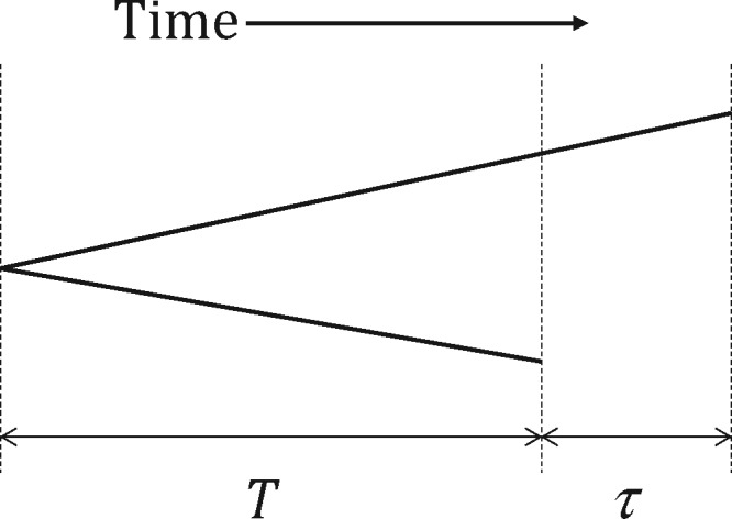
Coalescent tree of two viral sequences that are sampled at times different by τ. Assuming a constant rate µ of neutral (synonymous) mutation along a lineage, the expected neutral sequence difference is given by $(2E\left[T\right]+\tau )\mu$, where T is time to the coalescence of two contemporaneous sequences. Therefore, the expectation of synonymous sequence difference is greater than the scaled mutation rate, 2E[T]µ = 2 N_eµ, and the difference is τµ.

This problem can also be expressed as a difficulty in measuring allele frequencies from serially sampled sequences. Imagine that new sequence variants either rapidly drift to extinction or increase rapidly within flu seasons, as expected for small N_e, such that their frequencies are either low or high at a given time in the population. Suppose sequences were steadily sampled over several months and, in the middle of this period, a new variant rapidly increased from low to high frequency in the population. In that case, this allele is erroneously estimated to be in an intermediate frequency during this time interval, thus yielding high heterozygosity. Conversely, if this allele started from an intermediate frequency but became fixed in the middle of sampling interval, then allele frequency is overestimated and heterozygosity is underestimated. Therefore, to estimate allele frequency correctly, it is necessary to set sampling-time intervals as narrow as possible. However, the minimum possible interval depends on how many and how evenly sequences are sampled over time per population.

For the same reason, the conventional summaries of the pattern of sequence polymorphism, such as Tajima’s D, the site-frequency spectrum, Wright’s F_ST, and the coefficients of linkage disequilibrium, are difficult to obtain for sequences with irregular sampling times because these statistics are defined in terms of allele/haplotype frequencies at a single time point. While covering several decades of influenza virus evolution, one can calculate these statistics only after dividing sequences into arbitrarily small time intervals, for example successive flu seasons (Bedford et al. 2011; Łuksza and Lässig, 2014), thus yielding the time series of statistics. It is not clear how such time series, which are unlikely to be independent of each other, should be combined to characterize the entire genealogical structure of the evolving influenza virus. A simple solution might be to obtain a single value by averaging the time series. Then again, an arbitrary decision on the number and length of sampling-time intervals may greatly influence those statistics.

In this study, we show that one can systematically summarize the genealogical structure of a rapidly evolving asexual population, without using arbitrary time intervals for grouping sequences, by correcting the sampling-time differences when measuring nucleotide differences between sequences. In particular, we propose a time-corrected mismatch distribution (TCMD) as an alternative to conventional statistics for quantifying genealogical structure, such as Tajima’s D or the site-frequency spectrum. Our approach is used to estimate parameters of an evolutionary model of influenza virus for the HA gene sequences of H3N2 subtype sampled over decades from different geographic regions. We use the model of a virus population undergoing recurrent positive selection (antigenic drift) together with complex metapopulation dynamics described in Kim and Kim (2016). In the end, we detected temporal shifts in the mutation rates of the HA and PB1 segments and found that recurrent positive selection is essential in shaping the genealogical structure of the HA segment.

Methods

Data

H3N2 viral sequences were downloaded from two databases, the NCBI Influenza Virus Resource (Bao et al. 2008; https://www.ncbi.nlm.nih.gov/genomes/FLU/Database) and GISAID (https://www.gisaid.org). We used only genome sets, namely entries that include the sequences of all viral segments (HA, NA, PB1, PB2, PA, NP, NS, and MP). In order to avoid overlapping samples from the two databases and/or potentially extracted from the same host on the same day, we retained only one sample among those with identical base sequences, regions, and dates. We also discarded a sequence if it contained a notation for a base other than A, C, G, and T in any position along the sequence or if the associated year, month, date, or region of extraction were not provided. We aligned only the coding region of each segment, and alignments were performed using the default parameters of the MAFFT program (Katoh et al. 2019; https://mafft.cbrc.jp/alignment/software). Finally, incomplete sequences for the coding region of segments were removed. At the end, we obtained a total of 6724 sequences for each segment from 1980 to 2017.

In all analyses that follow, samples from seasons 2007 to 2017 (from August 2007 to July 2017; the “10-year data”), corresponding to an alignment of 1441 sequences, were used. A season is defined to last from 1st August of 1 year to 31st July of the next year. Sequences from eight regions were analyzed: four from Northern Hemisphere [United States, England, China (including Hong-Kong, Macau, and Taiwan), and Japan], two from the Southern Hemisphere (Australia and Chile), and two from a tropical region (Nicaragua) and South East Asia (Thailand, Cambodia, and Vietnam). The number of samples for each region and season is highly variable and uneven. Therefore, we adjusted the sample sizes so that our 10-year data are comparable to data sets obtained by the simulations described below. When there were more than 40 samples for a region in a season, we randomly subsampled 40 sequences. If there were less than 10 samples, we removed the region for the season in our analyses. At the end, we obtained 10 adjusted sets containing between 10 and 40 sequences for each region in a season. Each of these 10-year data sets yields the alignment of 999 sequences. In the following, the “observed” value of a test statistic or distribution is the average over these 10 data sets whenever it is compared to the simulation result.

In addition, we used the alignment of 1157 sequences from 1980 to 2007 (the “27-year data”) for the joint analysis of mutation rate and nucleotide diversity. In this case, all sequences were used without dropping regions containing less than 10 sequences.

Influenza evolutionary model and computer simulation

To simulate viral sequences generated under the evolutionary conditions of seasonal influenza viruses, we use a metapopulation dynamic model developed by Kim and Kim (2016), in which viral sequences evolve under genetic drift, migration, and positive selection. A sequence has 1700 neutral (synonymous) biallelic sites, over which the level of sequence diversity is measured, and additional ε sites on which beneficial mutations increasing fitness by s, the selection coefficient, occur. These ε sites model the “epitope” sites on the HA gene that underlie the antigenic drift of influenza virus. Bidirectional mutation occurs with probability µ_g (=10⁻⁴) per generation per synonymous site and unidirectional mutation (from wild-type to beneficial) occurs with probability µ_g/3 per generation per epitope site. The total population is divided into eight subpopulations (demes), which undergo periodic cycles of extinction and recolonization, connected by migration. One year is divided into 80 viral generations. Four demes model geographic regions in the Northern Hemisphere. The carrying capacities (K) of these demes reach maximum (K_max) at the beginning/end of the year and remain at zero between the 28th and 54th generation (i.e., “summer”) of a year. Two demes model those in the Southern Hemisphere, having the opposite profile of carrying capacity, reaching K_max in the middle of a year. The remaining two demes maintain a constant carrying capacity K = 0.2 K_max (the “tropical” demes). More details about migration (parameterized by m) and reproduction under this metapopulation dynamics are described in Kim and Kim (2016). For each set of model parameters, the simulation runs for 40 years for 300 replicates and the first 30 years are removed as burn-in. Then, from the last 10 simulated years, we sample around 40 sequences per deme per year.

Basic statistics

Assume that n nonrecombining RNA or DNA sequences were sampled over time from a haploid population of effective size N_e. As illustrated in Figure 1, the synonymous difference d_ij between sequences i and j with the sampling-time difference τ_ij is expected to be $\mathrm{E}\left[d_{ij}\right]=2N_{\mathrm{e}}\mu +{\tau }_{ij}\mu$, where µ is the synonymous mutation rate, assuming that synonymous changes are neutral. (In this study, time is primarily counted in days. Therefore, µ is the mutation rate per day, unless stated otherwise. N_e is consequently defined as the size of an ideal Wright–Fisher population that reproduces once a day.) The above equation suggests that µ and N_e can be estimated by regression of d on τ: over the $\left(\begin{array}{c}n\\ 2\end{array}\right)$ points of (τ, d), the slope of regression line is the estimate of mutation rate, $\widehat{\mu }$. Then, the sampling-time-corrected nucleotide difference between sequences i and j is given by:

$${\check{d}}_{ij}=d_{ij}-\widehat{\mu }{\tau }_{ij},$$ (1)

and the corrected mean pairwise sequence differences, $\check{\pi }$, is obtained as the arithmetic mean of all ${\breve{d}}_{ij}$ or, equivalently, as the y-intercept of the above regression. If two sequences were sampled too far apart in time (namely, T ≪ τ in Figure 1), the nucleotide difference in such a pair might have little information about the coalescent process. Therefore, $\check{\pi }$ can be optionally calculated using only the subset of sequence pairs that satisfy τ < τ_max. Synonymous sequence differences for each pair of sequences (d_ij) in a segment of the H3N2 virus are obtained according to the method of Nei and Gojobori (1986) implemented in CodeML in the PAML package (Yang 1997, 2007). From $\widehat{\mu }$ and $\check{\pi }$, we can define the estimate of (coalescent) effective population size, $\widehat{N_{\mathrm{e}}}=\check{\pi }/\left(2\widehat{\mu }\right)$.

Alternative estimates of µ can be obtained either by plotting sequence divergence from the oldest sequence in the sample against the corresponding sampling-time difference, in which case the mutation rate is estimated as the slope of the regression line, or by using a phylogenetic method that jointly infer tree topology and mutation rate over the branches. For the latter, we used the software BEAST (Drummond et al. 2012). Both methods were applied to simulated data so that the accuracies of estimation could be estimated. We ran BEAST analysis for each replicate of the simulated data for 3,000,000 generations, sampling every 500 generations following a burn-in period of 300,000 generations. The results were analyzed using Tracer.v1.7.1 (Rambaut et al. 2018), and µ was estimated as the mean of the posterior distribution.

Next, assuming that the population under consideration is subdivided into D demes, Wright’s F_ST can be defined for serially sampled data, by applying the above sampling-time correction to Nei’s G_ST (Nei 1973). Let π_l be the arithmetic mean of $\check{d}$ for all pairs of sequences found in deme l. Here, $\check{d}$ in this specific deme is still calculated using Equaiton (1) with $\widehat{\mu }$ that was first determined using all sequences from all demes. Similarly, π_lk is defined as the arithmetic mean of all ${\check{d}}_{ij}$ where sequence i is from deme l and sequence j from deme k. Then,

$$\begin{array}{c}{\pi }_{\mathrm{S}}=\sum _{l=1}^D{\pi }_l/D\\ {\pi }_{\mathrm{T}}=\left(\sum _{l=1}^D{\pi }_l+2\sum _{l<k}{\pi }_{lk}\right)/D^2\end{array}$$

and

$$F_{\mathrm{ST}}=1-\frac{{\pi }_{\mathrm{S}}}{{\pi }_{\mathrm{T}}}.$$ (2)

This approach allows one to summarize the degree of genetic differentiation between subpopulations into a single value, even for data that spans a long evolutionary period. However, reminding the definition of Wright’s F_ST and its genealogical interpretation (Slatkin and Hudson 1991), we realize that π_S should quantify the level of polymorphism in sequences that are not only sampled in the same subpopulations but also at the same (or nearly same) time. With limited migration, the lineages of two sequences are expected to coalesce faster if they are sampled from the same deme than from different demes. As a result, π_S < π_T, and thus F_ST > 0. However, if two sequences from a local population are sampled with a large time difference, a more recently sampled lineage is likely to have migrated to other demes by the time the other lineage is sampled. Then, their coalescent time may be no shorter than those sampled from different demes. Therefore, F_ST by Equation (2) will approach zero regardless of population subdivision as more sequence pairs with large τ are included. This is particularly true for H3N2 viruses that are globally exchanged through seasonal movements, mostly between the Northern and Southern Hemispheres. Therefore, we calculate π_S and π_T using only sequence pairs that are sampled within τ_max = 300 days (see Results).

Bootstrap tests of intersegmental differences

Three statistics described above $\widehat{\mu }$, $\check{\pi }$, and $\widehat{N_{\mathrm{e}}}$ were calculated for six segments (HA, NA, PB1, PB2, PA, and NP) of H3N2 data. To test if these estimates are significantly different between segments, we use a bootstrap test. Let ${\widehat{X}}_A$ and ${\widehat{X}}_B$ be the estimates of a parameter X from segments A and B. Then we define $\widehat{\theta }=|{\widehat{X}}_A-{\widehat{X}}_B|$ and test if it is significantly greater than zero. Under the null hypothesis (${\theta }_0=\left|X_A-X_B\right|=0$), $\widehat{\theta }-{\theta }_0$ is drawn from a distribution that can be approximated by the distribution of ${\widehat{\theta }}^{\mathrm{*}}-\widehat{\theta }$, where ${\widehat{\theta }}^{\mathrm{*}}=|{\widehat{X}}_A^{\mathrm{*}}-{\widehat{X}}_B^{\mathrm{*}}|$ is a bootstrap value of $\widehat{\theta }$. Then, the P-value is approximately the proportion of bootstrap samples that satisfy ${\widehat{\theta }}^{\mathrm{*}}-\widehat{\theta \mathrm{ }}>\widehat{\theta \mathrm{ }}-{\theta }_0=\widehat{\theta \mathrm{ }}$ (following the “first guideline” of Hall and Wilson 1991). A pseudo-data set is prepared by randomly sampling triplet-codon columns in the alignment of a given segment with replacement until it has the same number of codons as the original sequence. For the bootstrap test, 1000 pseudo-data sets for each segment pair were generated. Using the same method, we can also perform a bootstrap test to compare X from two different sets (e.g., old vs recent sequences) of a single segment.

TCMD for HA segment

Rogers and Harpending (1992) pointed out that the distribution of pairwise sequence differences in a sample, a mismatch distribution, reflects the genealogical (coalescent) structure of sampled (nonrecombining) sequences and can thus be used to infer the underlying evolutionary processes. We propose that the distribution of$\mathrm{ }{\breve{d}}_{ij}$ in Equation (1) similarly reveals the genealogical structure of nonrecombining sequences that were serially sampled in time. We call it a TCMD. Then, TCMDs obtained from actual and simulated data are compared to find the best-fit parameter values of our evolutionary model (see below). We use the Kolmogorov–Smirnov (KS) test in R (Marsaglia et al. 2003) to calculate the statistical significance of the difference between TCMDs.

Data availability

The C codes and R scripts for the above simulation and analyses, and sequence alignments are available from https://github.com/YuseobKimLab. Supplemental Material available at figshare: https://doi.org/10.25386/genetics.13271732.

Results

Comparison of methods for mutation rate estimation

We first evaluated the performances of three methods of estimating µ: regression based on all pairwise sequence differences (the method proposed in this study), regression based on differences between the oldest and all the other sequences (“conventional regression”), and the Bayesian phylogenetic method implemented in BEAST. We generated 300 replicates of simulation using parameters [ε = 40, m = 0.0009, K_max = 900, and most importantly µ = 2.19 × 10⁻⁵ per day (µ_g = 10⁻⁴)] that generate sequence diversity and sampling time distributions similar to those observed in the 10-year HA data. Only neutrally evolving (“synonymous”) sites in simulated data were used for inference. The mean (the 2.5th/97.5th quantile) of $\widehat{\mu }$ (×10⁻⁵) obtained by our method is 2.09 (1.47/2.80). We obtained a similar result with conventional regression: 2.09 (1.55/2.88). BEAST returned higher estimates: 2.49 (2.13/2.55). Therefore, given the simulation parameter (2.19), regression methods generated smaller biases than BEAST, but BEAST yielded more consistent estimates. As expected, far longer computational time was required for BEAST than for regression methods.

Estimation of population genetic parameters

Using the method of correcting differences in sampling times, we jointly estimated mutation rate ($\widehat{\mu }$) and mean pairwise synonymous difference ($\check{\pi }$) for all segments of H3N2 viruses, except for MP and NS that have overlapping protein-coding sequences and thus a small number of unconstrained synonymous sites. We analyzed data sets of viral genomes for either 27 years (1980 − 2007), the subsequent 10 years (2007 − 2017), or the combined 37 years (1980 − 2017). In the following, we simply call them 27-, 10-, or 37-year data, respectively. The $\widehat{\mu }$ values range from 1.3 × 10⁻⁵ to 3.19 × 10⁻⁵/site/day over different segments and data sets (Table 1 and Figure 2). The HA segment yields the largest estimates of $\widehat{\mu }$ in all data sets, and PB1 has the second largest for 27- and 37-year data but not for the recent 10 years. To examine if these differences in $\widehat{\mu }$ among segments are significant, we performed bootstrap tests, as described in Methods, for all pairs of segments (Supplementary Table S1). A significant difference was not found in the recent 10 years (P > 0.05 for all paired comparisons). However, using 27- and 37-year data, we find that the $\widehat{\mu }$ of HA is significantly higher than other segments, but not against PB1 in the 37-year data. In addition, we notice that $\widehat{\mu }$ for the recent 10 years is generally smaller than for the preceding 27 years. We thus applied the same bootstrap method to compare mutation rates between the 10- vs 27-year data sets. We find a significant difference only for HA (Figure 2).

Table 1.

Sampling-time corrected, mean pairwise (synonymous) nucleotide difference, $\check{\pi }$, the estimate of mutation rate µ (per day), and the estimate of effective population size N_e for 27-year (1980–2007), 10-year (2007–2017), and 37-year (1980–2017) H3N2 data sets

	27-year (1980–2007)			10-year (2007–2017)			37-year (1980–2017)
Segment	$\widehat{\mu }$(×10−5)	$\check{\pi }$	$\widehat{N_{\mathrm{e}}}$	$\widehat{\mu }$(×10−5)	$\check{\pi }$	$\widehat{N_{\mathrm{e}}}$	$\widehat{\mu }$(×10−5)	$\check{\pi }$	$\widehat{N_{\mathrm{e}}}$
HA	3.19	0.0318	497	1.99	0.0296	742	3.04	0.0219	361
	(2.46/4.05)*	(0.0225/0.0427)*	(318/730)*	(1.19/2.90)*	(0.0241/0.0355)	(502/1214)	(2.38/3.77)	(0.0149/0.0288)	(220/533)
PB1	2.20	0.0513	1165	1.75	0.0366	1029	2.50	0.0399	798
	(1.68/2.75)	(0.0398/0.0635)	(812/1674)	(1.17/2.62)	(0.0315/0.0422)	(719/1606)	(1.98/3.03)	(0.0331/0.0471)	(619/998)
PB2	1.85	0.0542	1468	1.83	0.037	1013	2.09	0.0415	993
	(1.34/2.40)	(0.0423/0.0663)	(1030/2152)	(1.16/2.54)	(0.0318/0.0419)	(733/1560)	(1.64/2.60)	(0.0348/0.0489)	(770/1300)
PA	1.82	0.051	1400	1.90	0.0308	812	1.99	0.0396	995
	(1.30/2.37)	(0.039/0.0645)	(923/2165)	(1.19/2.68)	(0.0255/0.0366)	(582/1270)	(1.54/2.49)	(0.0320/0.0470)	(748/1340)
NP	1.43	0.0585	2050	1.32	0.0311	1181	1.87	0.0391	1043
	(0.95/1.95)	(0.0444/0.0735)	(1335/3297)	(0.72/2.12)	(0.0248/0.0381)	(763/2080)	(1.38/2.41)	(0.0317/0.0470)	(778/1430)
NA	1.84	0.0505	1372	1.71	0.0256	747	1.90	0.0332	876
	(1.28/2.51)	(0.0356/0.0665)	(848/2087)	(1.34/2.90)	(0.0207/0.0312)	(468/1348)	(1.41/2.46)	(0.0254/0.0420)	(628/1220)

*Two-sided 95% confidence interval based on the distribution of estimates from 1000 bootstrap resampling.

Figure 2.

Pairwise nucleotide difference (d) per site of segments HA, NA, PB1, PB2, PA, and NP plotted against sampling time difference (τ, in days) for H3N2 data sequences. Data points are from 27-year data (1980–2006; black dots) and from the 10-year data (2007–2017; gray dots). Regression lines for 27- and 10-year data are shown in red and blue, respectively. The proportions of bootstrap samples in the tests for the statistical difference between 27- and 10-year periods of $\widehat{\mu }$, $\stackrel{⌣}{\pi }$, and $\widehat{N_e}$ are shown below each regression plot.

The level of synonymous polymorphism ($\check{\pi }$) is also variable across segments. From this, we may infer the intensities of natural selection that differentially reduce the sequence diversities of segments by hitchhiking effects. However, because differences in $\check{\pi }$ might also arise due to differences in µ, we assess the effect of selection by the estimate of effective population size, $\widehat{N_{\mathrm{e}}}=\check{\pi }/\left(2\widehat{\mu }\right)$. The $\widehat{N_{\mathrm{e}}}$ of the HA segment (= 361) is smaller than half of the other segments in the 37-year data (P < 0.008 against NA and P < 0.002 against all other segments in bootstrap tests; Table 1, Supplementary Table S1), as expected for this segment that is known to undergo recurrent selective sweeps (antigenic drift). Note that, as the unit of time we use (for τ and, thus, $\widehat{\mu }$) is a day, $\widehat{N_{\mathrm{e}}}$ = 361 means that two random HA sequences existing at a given time during the 37-year period coalesced in 1 year on average. We observe similar results in the 27-year data, with $\widehat{N_{\mathrm{e}}}=497$. Interestingly, the N_e of HA segment is estimated to be about twice larger for the recent 10 years than estimated for the entire 37 years. The $\widehat{N_{\mathrm{e}}}$ of the NA segment is smaller than those of non-HA segments in the recent 10 years but not in the 27- or the entire 37-year data sets.

The above results were obtained by calculating synonymous differences for all pairs of sequences in a data set, regardless of differences in sampling times (τ). Using sequence pairs that are not far apart in sampling times (i.e., τ < τ_max) resulted in virtually identical estimates of $\check{\pi }$ using HA sequences of the 10-year data or the corresponding simulation data (Supplementary Figure S1).

Next, we calculated the sampling-time-corrected F_ST, as describe in Methods, for HA sequences of the 10-year data. It slightly increases from 0.15 to 0.23 as we impose the decreasing limit of sampling time differences (τ_max) (Supplementary Figure S1). In contrast, F_ST calculated for an equivalent 10-year data set obtained from simulation with a clear population structure (Supplementary Figure S2) increases more rapidly as we decrease τ_max, consistent with the nature of F_ST (see Methods). This discrepancy between actual and simulated data occurs because H3N2 sequences are very unevenly distributed over different regions and years: as the mean within-population sequence difference, π_S, is obtained largely from pairs within a few region-year, decreasing τ_max does not have a large effect on π_S. In principle, π_S should be obtained from pairs of sequences that existed close in time or in the same flu season. Therefore, in the following, we calculate F_ST imposing τ_max = 300 days, because, in the analysis using simulated data, τ_max = 300 produced values similar to those obtained using sequence pairs sampled within the same 6-month-old flu season (Supplementary Figure 2).

TCMD and population genetic inferences

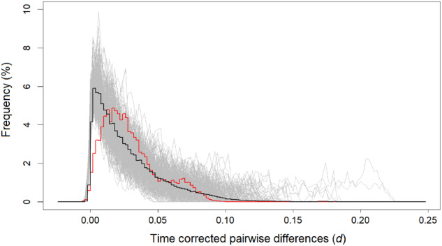
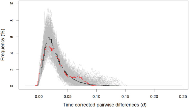
As an alternative to Tajima’s D or the site-frequency spectrum, which cannot be applied to a long, irregular time series of sequences, this study proposes the TCMD (i.e., the distribution of ${\breve{d}}_{ij}$) for quantifying the genealogical structure of an evolving population. We obtained TCMDs for six viral segments (two segments with an insufficient number of synonymous sites, NS and MP, are not included) using either 27- or 10-year data (Figure 3). In the former data set, the TCMD of the HA segment is distinctly different from the other viral segments, having more sequence pairs with small synonymous differences (Figure 3A), consistent with the significantly smaller estimate of N_e (Table 1). Other segments exhibit TCMDs that are similar overall but look rather noisy, particularly toward right tails. However, by comparison, we find less fluctuation and smaller inter-segmental differences in the TCMDs of sequences from the recent 10 years (Figure 3B). This is likely because a much larger number of viruses were sampled in recent years than before: we averaged the TCMDs of 10 sets of subsampled sequences (see Methods). In this recent period, NA stands out from the other five segments for having more sequence pairs with smaller differences, albeit the difference is very small. Similar TCMDs for these six segments suggest that their evolutionary dynamics are subject to common population genetic factors, even though a certain degree of independence is expected due to reassortment between segments (Holmes et al. 2005; Berry et al. 2016). We also note in this 10-year data that the TCMD curves of all segments, except for NA, do not decrease monotonically but have small peaks or “bumps” at the right tail (close to ${\breve{d}}_{ij}$ = 0.1; see Discussion).

Figure 3.

The TCMDs of six influenza virus segments in the 27-year (A) and 10- year (B) H3N2 data sets. To obtain $\stackrel{⌣}{d}$ and make histograms ${\tau }_{\max }=300$ and bin size w = 0.002 were used.

We then ask whether summary statistics and TCMD provide sufficient information about the evolutionary processes of viruses and thus allow us to find the best-fit model and its parameter values. As a starting point, this study focuses on the model of HA sequence evolution proposed in Kim and Kim (2016) that includes the parameters of subpopulation extinction/recolonization, migration, and recurrent positive selection (see Methods). We performed individual-based computer simulation under this model using diverse sets of parameter values and searched values producing $\check{\pi }$, F_ST, and TCMD that match those obtained from HA sequences sampled in recent 10 years.

Sequences under neutrality (ε = 0 thus no positive selection) were first generated by simulation with various combinations of K_max and m. However, no parameter set was found to yield $\check{\pi }$ and F_ST simultaneously close to the values obtained from actual HA sequences (Supplementary Table S2). For all parameter values examined, the TCMD also did not match the TCMD of the actual data (Figure 4). We thus tentatively conclude that demographic processes alone cannot explain the pattern of HA sequence diversity in the last 10 years.

Figure 4.

The average TCMD (black curve) for simulated data under neutrality (s = 0) with m = 0.004 and $K_{\max }=110$ that produce the best-fitting $F_{\text{ST}}$ and $\stackrel{⌣}{\pi }$ values to the observed data (red curve; the TCMD of HA segments in the 10-year data set). TCMDs of individual simulation replicates are shown in gray curves. To obtain $\stackrel{⌣}{d}$ and make histograms ${\tau }_{\max }=300$ and w = 0.002 were used.

Adding positive selection greatly improved the fit of simulation to data (Figure 5, Supplementary Figures S3 and S4). Using s = 0.05 or 0.1 (values in the range compatible with the temporal change of allele frequencies at known antigenic variant sites; Kim and Kim 2016), we assumed the number of epitope sites ε = 10, 20, 30, or 40. Given that per-site µ is fixed, ε determines the rate of beneficial mutation. For each combination of s and ε, we first coarse-searched values of K_max and m, in the range of values shown in Supplementary Table S2, until a close agreement in $\check{\pi }$ and F_ST between the actual and simulated data was obtained. Then, further fine adjustments of K_max and m within narrowed-down intervals were made to find the best fit TCMD using a grid search at the resolution of two significant digits for both K_max and m. (Therefore, in the following, “best-fit” parameter set means one that returns the largest P-value of KS test among points on the grid.) For an increasing value of ε, the best fit was obtained with increasing K_max and decreasing m (Table 2). How responsive the shape of TCMD is to the changes of K_max and m is shown in Supplementary Figure S5.

Figure 5.

The average TCMD (black curve) for simulated data under positive selection (s = 0.1 and ε = 10) with m = 0.00025 and $K_{\max }=6700$, which is congruent to the TCMD (red curve) of HA segment in the 10-year H3N2 data (KS test, p = 0.058). TCMDs of individual simulation replicates are shown in gray curves. To obtain $\stackrel{⌣}{d}$ and make histograms ${\tau }_{\max }=300$ and w = 0.002 were used.

Table 2.

Parameters and best-fitting results of the metapopulation model under neutrality (s = 0) and positive selection (s = 0.05 and 0.1)

s	0	0.05				0.1
ε	0	10	20	30	40	10	20	30	40
K max	110	250	440	690	900	6,700	14,000	32,000	50,000
m	0.004	0.0024	0.0015	0.0011	0.0009	0.00025	0.00017	0.00013	0.00011
$\check{\pi }$	0.0304	0.0297	0.0283	0.029	0.029	0.0287	0.0283	0.029	0.0292
F ST	0.1564	0.1657	0.1621	0.1606	0.1609	0.1576	0.1641	0.1619	0.1561
KS*	7.74e-12	0.0003	0.0098	0.0007	0.0421	0.058	0.021	0.0007	0.0144

*P-value of KS test.

The quantitative measurement of agreement between the TCMDs of simulated data (averaged over replicates) and the actual data was given by the P-value of KS test, the null hypothesis of which assumes the identity of two distributions. We found p > 0.05 (thus agreement between simulation and data) for one parameter set: s = 0.1, ε = 10, K_max = 6700 and m = 0.00025 (Figure 5). The second best fit (P = 0.041) was obtained with s = 0.05, ε = 40, K_max = 900 and m = 0.0009. The best-fit TCMDs for each set of s and ε (Table 2) are shown in Supplementary Figures S3 and S4. For a given s, the best-fit TCMDs appear to be similar across different values of ε upon visual inspection, necessitating the quantitative evaluation of fits by the KS test. To obtain TCMDs here, for both simulated and actual data, we used ${\breve{d}}_{ij}$ for pairs whose sampling-time differences are less than τ_max = 300 days and the bin size w = 0.002. Changes from this scheme uniformly increased or decreased P-values in the KS tests. However, we consistently found the above sets of parameter values the best-fitting ones.

Further simulations were performed with less frequent beneficial mutations (ε = 2 and 5) while adjusting other parameters to generate close-fitting $\check{\pi }$ and F_ST. As expected, TCMDs obtained from these simulations are intermediate between that of the best-fit neutral model and those of selection with frequent positive selection (ε ≥ 10) (Supplementary Figure S6). Therefore, the TCMD was highly informative in detecting positive selection but of rather limited use in estimating ε. Namely, with ε varying in the range of large values (>10), the genealogical structure of a segment in our model, captured by TCMD, could be made to fit the HA sequence data reasonably well by adjusting other parameters.

Discussion

In this study, we used nonuniformly serial-sampled sequences of influenza A/H3N2 viruses from public databases (GISAID and NCBI) to calculate µ for different segments (HA, NA, PA, PB, PB2, and NP). We calculated synonymous differences (d_ij), with the sampling-time difference τ_ij, in all pairs of sequences in our data sets and used the linear regression to estimate the synonymous mutation rate. Conventionally, the linear regression was used to calculate viral mutation rates but by comparing sequences to a close outgroup or an oldest sequence in the sample, such as for HIV-1 (Lukashov and Goudsmit 1998) and SARS-CoV2 (https://nextstrain.org/ncov/global?l=clock). We found that this method performs similar to ours when tested against the 10-year data. However, by explicitly incorporating the coalescent process in our linear regression our method could also jointly estimate π, and thus, N_e. One may also estimate the mutation rate using the methods of phylogenetic tree inference, in which the mutation rate is one of parameters that are jointly estimated. However, this approach is very time-consuming with a large number of sequences, unclear regarding how uncertainty in tree structure would affect the accuracy of the mutation rate estimation, and limited to a nonrecombining DNA/RNA segment that allows tree reconstruction. Our approach is straightforward and can be applied to recombining sequences (e.g., viruses undergoing homologous recombination).

We estimated the mutation rates of H3N2 viral segments to range from 1.3 × 10⁻⁵ to 3.19 × 10⁻⁵/site/day. These results are similar to the estimates of synonymous substitution rate found by previous studies. For example, Hanada et al. (2004) estimated the average synonymous substitution rate of 6.84 × 10⁻³/site/year (≈1.87 × 10⁻⁵/site/day) when all human influenza A virus were combined. Interestingly our estimate of synonymous mutation rate on HA between 1980 and 2007 is significantly higher compared to other segments in the same period and against the same segment between 2007 and 2017. A significant difference between the two periods is not observed in other segments. PB1 shows a similar trend of $\widehat{\mu }$, although the estimate in the 27-year data is significantly higher only against NP (Table 1). While it was clearly demonstrated that the HA gene evolves rapidly under recurrent positive selection on nonsynonymous variants (i.e., antigenic drift; Nelson and Holmes 2007; Rambaut et al. 2008; Bhatt et al. 2011), the elevation of synonymous substitution rates in this gene needs an explanation.

One possibility is that synonymous sites on the influenza viral genome are not completely neutral but under weak constraints resulting from codon usage bias or formation of the secondary structure of the single-stranded RNA segments, which slows down the substitution rate relative to the rate expected under complete neutrality. Then, recurrent positive selection on linked nonsynonymous sites interferes with such weak selection (i.e., reduces effective population size) and can therefore increase the rate of substitutions at synonymous sites (Sharp and Li 1987). This hypothesis implies that recurrent positive selection on HA was more frequent between 1980 and 2007 than between 2007 and 2017. We note that the significantly smaller $\widehat{N_{\mathrm{e}}}$ for the HA segment in 1980–2007 than in 2007–2017 (Table 1) is compatible with more frequent positive selection in the former period.

The violation of the neutrality assumption on synonymous sites should also influence other aspects of our inferences. The reduced rate of synonymous substitutions would lead to underestimating mutation rate (thus, the overestimation of N_e). Considering that new mutations at the weakly selected sites are more likely to be slightly deleterious than advantageous, those mutations would be mapped preferentially on the outer (terminal) lineages, thus distorting the structure of genealogy by extending outer branches. However, we do not observe a pattern (other than a temporal change in $\widehat{\mu }$ of HA and PB1) that suggests a sweeping violation of neutrality at synonymous sites in the H3N2 population. One can imagine that substitutions at a synonymous site under selection may occur from the wild-type allele to a slightly deleterious allele (by genetic drift) and, later, back to the wild-type allele. Then, the divergence of synonymous sequences may decelerate due to multiple hits. We do not find such a deceleration in synonymous divergence over time (Table 1, Figure 2): clock-like sequence evolution is observed on segments other than HA and PB1. This result therefore seems to suggest that the majority of synonymous sites evolve under neutrality. Nonetheless, further analysis, for example following up the fates of synonymous variants at various frequencies (Zanini and Neher 2013), is required to accurately evaluate the neutrality of synonymous changes in H3N2 viruses.

An alternative explanation for the elevated mutation rates of HA and PB1 segments before 2007 may be found by noting that, at the origin of H3N2 virus, these segments came from the avian influenza virus and all other segments from human H2N2 (Wendel et al. 2015; Allen and Ross 2018). Then, evolutionary changes on HA and PB1 might have been faster during the early period of adaptation to a new host, explaining the lower effective population sizes and higher synonymous mutation rates of these segments before 2007 than after. Codon usages, secondary structures, or G + C content of HA and PB1 might have evolved faster, directly increasing the rates of synonymous substitutions, in their early adaptation to new host (Dos Reis et al. 2009). Indeed, we find that the G + C content of HA decreased over time and the rate of this change was greater before 2007 and less after (Supplementary Figure S7).

We also applied sampling-time corrections to obtain an F_ST statistic and mismatch distribution that can measure the genealogical structure of a population from irregular time series of nucleotide sequences. Our F_ST statistic is moderately dependent on τ_max, which, in principle, should be minimized. In practice, if multiple sequences from each deme under consideration are available at similar time points, say less than 3 months apart for seasonal influenza viruses, this restriction on τ_max should not be a problem. Our estimate of F_ST (≈0.16) confirms the earlier results that, despite rapid global circulation, HA sequences of H3N2 viruses are genetically differentiated over geographic regions. It indicates that despite rapid viral transmission across regions (“migration” rate in our model), genetic drift within each region is relatively stronger.

Modifying the mismatch distribution of Rogers and Harpending (1992), we proposed the TCMD as an alternative to Tajima’s D statistic or the site-frequency spectrum that were defined for sequences sampled at one time point (or at nearly identical time points in the coalescent time scale). A TCMD captures the genealogical structure of population and thus provides information for finding the fitting parameters of a population genetic model. Although TCMD itself is not a single summary statistic, congruence, or distance between TCMDs, particularly between TCMDs of actual and simulated data, can be easily measured for parameter estimation. However, as our individual-based simulation for the joint demographic-selection model of the H3N2 virus is highly time-consuming, the entire parameter space of the model could not be systematically explored, for example, through approximate Bayesian computation. It was particularly difficult to perform simulations with s = 0.15 because a close fit was obtained only with very large K_max (>50,000), under which simulation took several weeks for one parameter set. (We find such a large K_max with s = 0.15 unrealistic anyway, because the N_e of H3N2 under which new beneficial alleles arise should be small enough to suppress soft selective sweeps; Kim and Kim 2016). Consequently, we decided not to continue the analysis for s = 0.15.

We attempted to find the best-fit TCMD for each set of chosen s and ε by making a limited grid search of demographic parameters (K_max and m) only. Therefore, further simulations with more rigorous optimization algorithm will probably reveal different sets of parameters that yield better agreement with the observed data. Even further improvement in inference will likely depend on proposing a qualitatively different model that incorporates important evolutionary processes determining the evolutionary dynamics of H3N2 viruses not considered here. For instance, we find from the visual inspection of evolutionary trees for HA sequences in the last 10 years that a considerable proportion of sequence pairs are highly divergent (thus, the “bump” near the right tail of TCMD; Figure 3). This observation might indicate the presence of an evolutionary force that promotes the coexistence of two divergent HA lineages.

The methods developed here can be generally applied to serially sampled population genetic data. We inferred population genetic parameters separately for each influenza virus segment, which, not undergoing recombination, is a natural unit of independent evolution. However, our methods, including TCMD, can be applicable to recombining sequences as well. We think that correct inference can be made as long as a simulation that generates data with the matching rate of recombination is used. This approach could lead, for example, to the evolutionary analysis of other RNA viruses undergoing homologous recombination, such as SARS-CoV-2, whose sequences were also nonuniformly serial sampled.

Funding

This research was supported by the National Research Foundation (NRF) grants 2018M3A9H4055197 and 2020R1A2C1009261 funded by the Korean government.

Conflicts of interest: None declared.

Literature cited

- Allen JD, Ross TM. 2018. H3N2 influenza viruses in humans: viral mechanisms, evolution, and evaluation. Hum Vaccin Immunother. 14:1840–1847. [DOI] [PMC free article] [PubMed] [Google Scholar]
- Bao Y, Bolotov P, Dernovoy D, Kiryutin B, Zaslavsky L, et al. 2008. The influenza virus resource at the National Center for Biotechnology Information. JVI 82:596–601. [DOI] [PMC free article] [PubMed] [Google Scholar]
- Bedford T, Cobey S, Pascual M. 2011. Strength and tempo of selection revealed in viral gene genealogies. BMC Evol Biol. 11:220. [DOI] [PMC free article] [PubMed] [Google Scholar]
- Berry IM, Melendrez MC, Li T, Hawksworth AW, Brice GT, et al. 2016. Frequency of influenza H3N2 intra-subtype reassortment: attributes and implications of reassortant spread. BMC Biol. 14:117. [DOI] [PMC free article] [PubMed] [Google Scholar]
- Bhatt S, Holmes EC, Pybus OG. 2011. The genomic rate of molecular adaptation of the human influenza A virus. Mol Biol Evol. 28:2443–2451. [DOI] [PMC free article] [PubMed] [Google Scholar]
- Bollback JP, York TL, Nielsen R. 2008. Estimation of 2Nes from temporal allele frequency data. Genetics. 179:497–502. [DOI] [PMC free article] [PubMed] [Google Scholar]
- Bragstad K, Nielsen LP, Fomsgaard A. 2008. The evolution of human influenza A viruses from 1999 to 2006: a complete genome study. Virol J. 5:40. [DOI] [PMC free article] [PubMed] [Google Scholar]
- Dos Reis M, Hay AJ, Goldstein RA. 2009. Using non-homogeneous models of nucleotide substitution to identify host shift events: application to the origin of the 1918 ‘Spanish’ influenza pandemic virus. J Mol Evol. 69:333–345. [DOI] [PMC free article] [PubMed] [Google Scholar]
- Drummond AJ, Suchard MA, Xie D, Rambaut A. 2012. Bayesian phylogenetics with BEAUti and the BEAST 1.7. Mol Biol Evol. 29:1969–1973. [DOI] [PMC free article] [PubMed] [Google Scholar]
- FDA. 2020. https://www.fda.gov/food/whole-genome-sequencing-wgs-program/genometrakr-network.
- Ferrer-Admetlla A, Leuenberger C, Jensen JD, Wegmann D. 2016. An approximate Markov model for the Wright-Fisher diffusion and its application to time series data. Genetics. 203:831–846. [DOI] [PMC free article] [PubMed] [Google Scholar]
- Fitch WM, Bush RM, Bender CA, Cox NJ. 1997. Long term trends in the evolution of H(3) HA1 human influenza type A. Proc Natl Acad Sci U S A. 94:7712–7718. [DOI] [PMC free article] [PubMed] [Google Scholar]
- Fitch WM, Leiter JM, Li XQ, Palese P. 1991. Positive Darwinian evolution in human influenza A viruses. Proc Natl Acad Sci USA. 88:4270–4274. [DOI] [PMC free article] [PubMed] [Google Scholar]
- Good BH, McDonald MJ, Barrick JE, Lenski RE, Desai MM. 2017. The dynamics of molecular evolution over 60,000 generations. Nature. 551:45–50. [DOI] [PMC free article] [PubMed] [Google Scholar]
- Grenfell BT, Pybus OG, Gog JR, Wood JL, Daly JM, et al. 2004. Unifying the epidemiological and evolutionary dynamics of pathogens. Science. 303:327–332. [DOI] [PubMed] [Google Scholar]
- Hall P, Wilson SR. 1991. Two guidelines for bootstrap hypothesis testing. Biometrics. 47:757–762. [Google Scholar]
- Hanada K, Suzuki Y, Gojobori T. 2004. A large variation in the rates of synonymous substitution for RNA viruses and its relationship to a diversity of viral infection and transmission modes. Mol Biol Evol. 21:1074–1080. [DOI] [PMC free article] [PubMed] [Google Scholar]
- Holmes EC, Dudas G, Rambaut A, Andersen KG. 2016. The evolution of Ebola virus: insights from the 2013-2016 epidemic. Nature. 538:193–200. [DOI] [PMC free article] [PubMed] [Google Scholar]
- Holmes EC, Ghedin E, Miller N, Taylor J, Bao Y, et al. 2005. Whole-genome analysis of human influenza A virus reveals multiple persistent lineages and reassortment among recent H3N2 viruses. PLoS Biol. 3:e300. [DOI] [PMC free article] [PubMed] [Google Scholar]
- Katoh K, RozewickiJ, Yamada K D. 2019. MAFFT online service: multiple sequence alignment, interactive sequence choice and visualization. Briefings in Bioinformatics. 20:1160–1166. [DOI] [PMC free article] [PubMed] [Google Scholar]
- Kim K, Kim Y. 2016. Population genetic processes affecting the mode of selective sweeps and effective population size in influenza virus H3N2. BMC Evol Biol. 16:156. [DOI] [PMC free article] [PubMed] [Google Scholar]
- Lukashov VV, Goudsmit J. 1998. HIV heterogeneity and disease progression in AIDS: a model of continuous virus adaptation. Aids 12(Suppl A):S43–S52. [PubMed] [Google Scholar]
- Łuksza M, Lässig M. 2014. A predictive fitness model for influenza. Nature. 507:57–61. [DOI] [PubMed] [Google Scholar]
- Marsaglia G, Tsang WW, Wang J. 2003. Evaluating Kolmogorov’s distribution. J Stat Soft. 8:1–4. [Google Scholar]
- Nei M. 1973. Analysis of gene diversity in subdivided populations. Proc Natl Acad Sci USA. 70:3321–3323. [DOI] [PMC free article] [PubMed] [Google Scholar]
- Nei M, Gojobori T. 1986. Simple methods for estimating the numbers of synonymous and nonsynonymous nucleotide substitutions. Mol Biol Evol. 3:418–426. [DOI] [PubMed] [Google Scholar]
- Nelson MI, Holmes EC. 2007. The evolution of epidemic influenza. Nat Rev Genet. 8:196–205. [DOI] [PubMed] [Google Scholar]
- Rambaut A, Drummond AJ, Xie D, Baele G, Suchard MA. 2018. Posterior summarisation in Bayesian phylogenetics using Tracer 1.7. Syst Biol. 67:901–904. [DOI] [PMC free article] [PubMed] [Google Scholar]
- Rambaut A, Pybus OG, Nelson MI, Viboud C, Taubenberger JK, et al. 2008. The genomic and epidemiological dynamics of human influenza A virus. Nature. 453:615–619. [DOI] [PMC free article] [PubMed] [Google Scholar]
- Rogers AR, Harpending H. 1992. Population growth makes waves in the distribution of pairwise genetic differences. Mol Biol Evol. 9:552–569. [DOI] [PubMed] [Google Scholar]
- Schlötterer C, Kofler R, Versace E, Tobler R, Franssen SU. 2015. Combining experimental evolution with next-generation sequencing: a powerful tool to study adaptation from standing genetic variation. Heredity. 114:431–440. [DOI] [PMC free article] [PubMed] [Google Scholar]
- Schraiber JG, Evans SN, Slatkin M. 2016. Bayesian inference of natural selection from allele frequency time series. Genetics. 203:493–511. [DOI] [PMC free article] [PubMed] [Google Scholar]
- Sharp P, Li WH. 1987. The codon adaptation index-a measure of directional synonymous codon usage bias, and its potential applications. Nucl Acids Res. 15:1281–1295. [DOI] [PMC free article] [PubMed] [Google Scholar]
- Shu Y, Mccauley J. 2017. GISAID: Global initiative on sharing all influenza data from vision to reality. EuroSurveillance. 22:30494. [DOI] [PMC free article] [PubMed] [Google Scholar]
- Slatkin M, Hudson RR. 1991. Pairwise comparisons of mitochondrial DNA sequences in stable and exponentially growing populations. Genetics. 129:555–562. [DOI] [PMC free article] [PubMed] [Google Scholar]
- Slatkin M, Racimo F. 2016. Ancient DNA and human history. Proc Natl Acad Sci USA. 113:6380–6387. [DOI] [PMC free article] [PubMed] [Google Scholar]
- Steinrücken M, Bhaskar A, Song YS. 2014. A novel spectral method for inferring general diploid selection from time series genetic data. Ann Appl Stat. 8:2203–2222. [DOI] [PMC free article] [PubMed] [Google Scholar]
- Van den Bergh B, Swings T, Fauvart M, Michiels J. 2018. Experimental design, population dynamics, and diversity in microbial experimental evolution. Microbiol Mol Biol Rev. 82: [DOI] [PMC free article] [PubMed] [Google Scholar]
- Vitti JJ, Grossman SR, Sabeti PC. 2013. Detecting natural selection in genomic data. Annu Rev Genet. 47:97–120. [DOI] [PubMed] [Google Scholar]
- Wendel I, Rubbenstroth D, Doedt J, Kochs G, Wilhelm J, et al. 2015. The avian-origin PB1 gene segment facilitated replication and transmissibility of the H3N2/1968 pandemic influenza virus. J Virol. 89:4170–4179., [DOI] [PMC free article] [PubMed] [Google Scholar]
- Wille M, Holmes EC. 2020. The ecology and evolution of influenza viruses. Cold Spring Harb Perspect Med. a038489.10: [DOI] [PMC free article] [PubMed] [Google Scholar]
- Yang Z. 1997. PAML: a program package for phylogenetic analysis by maximum likelihood. Comput Appl Biosci. 13:555–556. [DOI] [PubMed] [Google Scholar]
- Yang Z. 2007. PAML 4: phylogenetic analysis by maximum likelihood. Mol Biol Evol. 24:1586–1591. [DOI] [PubMed] [Google Scholar]
- Zanini F, Neher RA. 2013. Quantifying selection against synonymous mutations in HIV-1 env evolution. J Virol. 87:11843–11850. [DOI] [PMC free article] [PubMed] [Google Scholar]
- Zinger T, Gelbart M, Miller D, Pennings PS, Stern A. 2019. Inferring population genetics parameters of evolving viruses using time-series data. Virus Evol. 5:vez011. [DOI] [PMC free article] [PubMed] [Google Scholar]
Associated Data
This section collects any data citations, data availability statements, or supplementary materials included in this article.
Data Availability Statement