

Abstract

The Joule–Thomson effect is a key chemical thermodynamic property that is encountered in several industrial applications for CO2 capture and storage (CCS). An apparatus was designed and built for determining the Joule–Thomson effect. The accuracy of the device was verified by comparing the experimental data with the literature on nitrogen and carbon dioxide. New Joule–Thomson coefficient (μJT) measurements for three binary mixtures of (CO2 + N2) with molar compositions xN2 = (0.05, 0.10, 0.50) were performed in the temperature range between 298.15 and 423.15 K and at pressures up to 14 MPa. Three equations of state (GERG-2008 equation, AGA8-92DC, and the Peng–Robinson) were used to calculate the μJT compared with the corresponding experimental data. All of the equations studied here except PR have shown good prediction of μJT for (CO2 + N2) mixtures. The relative deviations with respect to experimental data for all (CO2 + N2) mixtures from the GERG-2008 were within the ±2.5% band, and the AGA8-DC92 EoSs were within ±3%. The Joule–Thomson inversion curve (JTIC) has also been modeled by the aforementioned EoSs, and a comparison was made between the calculated JTICs and the available literature data. The GERG-2008 and AGA8-92DC EoSs show good agreement in predicting the JTIC for pure CO2 and N2. The PR equation only matches well with the JTIC for pure N2, while it gives a poor prediction for pure CO2. For the (CO2 + N2) mixtures, the three equations all give similar results throughout the full span of JTICs. The temperature and pressure of the transportation and compression conditions in CCS are far lower than the corresponding predicted Pinv,max and Tinv,max for (CO2 + N2) mixtures.
1. Introduction
The greenhouse gas (GHG) emissions identified as the culprit causing climate change have received worldwide attention. CO2 emissions are much higher than the limit recommended by scientists compared to other greenhouse gases.1 Carbon capture and storage (CCS) is arising as key technology that can effectively slow down the substantial increase in greenhouse gases.2 The captured CO2 transportation and storage are vital in the CCS process.3,4 The CO2 pipeline transportation is the most widely used transportation mode.5 The pressure loss along the pipeline is inevitable; thus, the Joule–Thomson effect is a key issue in pipeline transportation.6 The Joule–Thomson effect could be a contributing factor leading to a phase transition in the CO2 steam transportation. Once there are leakages in the pipeline,7 the temperature decrease caused by carbon dioxide flash and throttling expansion will cause brittle fracture of the pipeline due to supercooling. Another important aspect of the Joule–Thomson cooling in CCS is the geological storage process in which the impure CO2 stream would be injected into depleted hydrocarbon reservoirs or saline aquifers.8 The injection efficiency and formation permeability could be influenced by formation of hydrates due to significant Joule–Thomson cooling of the CO2 stream.9 The Joule–Thomson effect has been important thermodynamics in the study of the CCS applications.
Nitrogen is considered to be one of the most common impurities present with the captured carbon dioxide in the CCS process, which can greatly affect the thermodynamic properties of the CO2 stream and the efficiency of pipeline transportation.10 The research on the (CO2 + N2) mixtures mainly focuses on the thermodynamic properties relevant to CCS, such as density,11−13 vapor–liquid equilibrium,14,15 viscosity,16 etc. However, the work on the Joule–Thomson effect of (CO2 + N2) mixtures has not been reported.
At present, most of the research studies on the Joule–Thomson effect focus on pure substances such as N2, CO2, H2, Ar, He, CH4, C2H2, etc.17−27 Also, there are also a small number of binary and ternary mixtures’ Joule–Thomson effect reports.28−31 For binary systems, only (CO2 + CH4)32 and (CO2 + Ar)33 systems that contain the components relevant to CCS have been reported. Due to the difficulty in constructing experimental devices and measuring the Joule–Thomson effect, equations of state,34−36 molecular simulation,37−39 and computer software modeling40 have been popular with mathematical modeling on the Joule–Thomson effect, in recent years.
In this work, a reliable device was built for measuring the Joule–Thomson effect, proved with some reported data. Comprehensive μJT measurements were carried out for the binary mixtures of carbon dioxide with nitrogen (x(N2) = 0.05, 0.10, 0.5) at temperatures from 298.15 to 423.15 K with pressures up to 14 MPa. Moreover, three equations of state (GERG-2008, AGA8-92DC, PR) were used to calculate the μJT compared with the corresponding experimental values. The above three equations were used to evaluate the performance in predicting the JTIC for CO2 and N2, respectively. Also, a comparison was made between the predicted data and available data for the inversion curve of CO2 and N2. Besides, we also calculated the JTIC for (CO2 + N2) mixtures using the three EoSs.
2. Theoretical Background
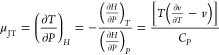
The temperature change caused by the pressure change is called the Joule–Thomson effect, and the μJT can be calculated according to the following formulas41
| 1 |
| 2 |
| 3 |
For H = H(T, P),
 |
4 |
 |
5 |
Equation 4 or 5 must be zero when we predict the Joule–Thomson inversion curve, and the common form can be obtained as eq 6(42)
| 6 |
The Joule–Thomson inversion curve (JTIC) is connected by the points in the P–T region, where the μJT is equal to 0. Also, the points in the curve divide the Joule–Thomson cooling region (μJT > 0) and Joule–Thomson heating region (μJT < 0).43
In this work, three equations of state including classical typical cubic state equation (PR EoS)44 and multiparametric equations (GERG-200845 and AGA8-92DC46 EoSs) were used to predict the μJT and JTICs. The detailed information of the three equations of state is given in the Supporting information.
3. Experimental Section
3.1. Chemicals
Carbon dioxide (purity ≥99.999%, cylinder number 12797179) and hydrogen (purity ≥99.999%, cylinder number 182084292) were purchased from Guangdong Huate Gas Co., Ltd. in Foshan, China. Also, critical parameters of the pure compositions were obtained from the NIST database47 for CO2 and N2. Three (CO2 + N2) binary mixtures were also supplied by Guangdong Huate Gas Co., Ltd., China. The molar composition (0.95 CO2 + 0.05 N2, cylinder number 206801101), (0.90 CO2 + 0.10 N2, cylinder number 206801059), and (0.50 CO2 + 0.50 N2, cylinder number 204114127) mixtures were prepared following the method of GB/T 5274-200848 (Chinese National Standards) and used without further purification.
3.2. Apparatus and Procedure
The μJT measurement device is schematically shown in Figure 1. The whole apparatus was divided into the following three parts: gas supply part, experimental section, and circulating pressurization part. The gas supply part provides gaseous mixtures from a specific cylinder with a volume of 40 L to a mass flowmeter monitoring the mass flow rate of gases. The gases then flow into a thermostatic heater, which could control the gas temperature. High-precision temperature sensors are set to monitor the temperature of gases. Temperature sensors have a temperature range of −173.15 to 523.15 K with a precision of ±0.1 K. When the gas temperature is constant, we could regulate the throttle valve to control the Joule–Thomson effect. The throttle valve is made of the splicing of large diameter pipelines and small diameter pipelines. To create a thermal insulation environment, a thick thermal insulation material should be attached to the throttle valve. Meanwhile, high-precision sensors were installed before and after throttling the experimental part. Each pressure sensor has a precision of ±0.01 MPa and a maximum range of up to 40 MPa. The entire pipeline is designed as a closed circuit and is circulated and supplied by a pneumatic compressor. The pneumatic booster pump is powered by an air compressor, which can provide a maximum boost of 0.7 MPa. The pneumatic booster pump has a maximum pressure of 25 MPa. A gas storage tank composed of two industrial gas cylinders is used to store mixed gas. Each cylinder has a volume of 40 L and pressures up to 15 Mpa.
Figure 1.

Schematic diagram of the μJT measurement apparatus: 1, gas cylinder; 2, three-way valve; 3, needle valve; 4, mass flowmeter; 5, needle valve; 6, numerical control thermometer; 7, temperature sensor; 8, needle valve; 9, pressure sensor; 10, Joule–Thomson valve; 11, temperature sensor; 12, pressure sensor; 13, three-way valve; 14, gas boost pump; 15, air supply compressor; 16, needle valve; 17, three-way valve; and 18, 19; gas storage.
The operation process for the μJT measurements is as follows: open the screws of cylinders #1, #18, and #19 to supply gases. We can adjust the flow of the gases by regulating needle valves #3 and #5. We must set the numerical control constant temperature heater in advance according to the experimental requirements. The temperature sensors #7 (T1) and #11 (T2) were set to monitor the temperature before and after the experimental throttling process. When the pressure and temperature reach the desired value, we could regulate the needle valve 8# and read the pressure value on pressure sensor #9 (P1). The values on temperature sensor #10 (T2) and pressure sensor #12 (P2) represent the temperature and pressure after throttling, respectively. In the experiment, to ensure that the experimental gas can be recycled, we need to turn on the pneumatic booster pump #14. Before starting the booster pump, we need to turn on the air compressor #15 to provide power.
Also, μJT can be calculated as
| 7 |
The uncertainty calculation method followed GUM.49 Temperature standard uncertainty uc(T) is given by the manufacturer of ±0.029 K. Taking into account the temperature calibration and drift, oscillation, etc., the expanded uncertainty in temperature U(T) is about 0.080 K (k = 2). Also, the pressure standard uncertainty uc(P) is ±0.0029 MPa. Also, considering the drift of calibration pressure, the expanded uncertainty in pressure U(P) is about 0.0070 MPa (k = 2). The standard uncertainties of μJT are further obtained based on the experimental variance of μJT in repeated measurements. The standard uncertainty uc(μJT) is 0.008 K·MPa–1 for CO2 and 0.005 K·MPa–1 for N2. Also, the absolute expanded uncertainties U(μJT) (k = 2) for all (CO2 + N2) mixtures are about 0.0017–0.0029 K·MPa–1.
4. Results and Discussion
4.1. Experiment System Verification
Within the scope of verifying the new self-built μJT measurement device, experiments on pure CO2 and pure N2 were carried out. We measured the μJT for pure CO2 in the range 303.15–423.15 K and pressures up to 14 MPa. At the same time, similar tests were carried out on N2 at 293.15–423.15 K and pressures between 0.1 and 14 MPa. The data for pure substances are compared with the existing relevant literature data21,50 and shown in Figure 2a,b. AAD is the average absolute deviation defined by eq 8; AA%D is the average absolute percentage deviation defined by eq 9. The AAD and AA%D for pure CO2 and N2 on μJT of experimental data from this work along with other literature data are shown in Tables 1 and 2.
| 8 |
| 9 |
As can be seen in Table 1, the experimental data for CO2 show desirable agreement with the experimental data reported by Roebuck et al. and Wang et al. The high AA%D between this work and Roebuck et al. data occurring in μJT is 1.5–2%, while it is 4–5% with Wang et al. data at 303.15 and 323.15 K. The data in the critical region have a higher deviation due to the drastic change in thermophysical properties. With an increase in temperature, the AA%D and AAD become smaller, which is also in line with the law reported by Wang et al. According to Wang, the deviations in the supercritical state and liquid state are larger than that of the gas state, and the deviation between average absolute errors between Wang and Roebuck is 4.93%.50 As shown in Table 2, the AAD between the N2-μJT data measured in this work and the existing one17 is small, about 0.1 K·MPa–1 in a wide range of temperature. The AA%D increased with increasing temperature, from 0.33% at 298.15 K to 1.58% at 423.15 K. It also can be seen from Figure 2 that our results are in good agreement with the N2-μJT and CO2-μJT data. Thus, the device we built highly meets the accuracy for experimental measurements.
Figure 2.

Comparison of μJT measured by this experimental system with data from the literature for (a) CO2.21,50 and (b) N2.17
Table 1. Average Absolute Deviation (AAD) and Average Absolute of Percentage Deviation (AA%D) between the μJT Values Measured for Pure CO2 in This Work and the Literature Data21,50.
| μJT data for CO2 | Roebuck
et al. |
Wang et al. |
||
|---|---|---|---|---|
| T/K | AA%D | AAD/K·MPa–1 | AA%D | AAD/K·MPa–1 |
| 303.15 | 2.01 | 0.12 | 4.28 | 0.07 |
| 323.15 | 1.48 | 0.08 | 5.87 | 0.26 |
| 373.15 | 0.67 | 0.03 | 1.26 | 0.07 |
| 398.15 | 0.70 | 0.03 | 2.43 | 0.12 |
| 423.15 | 0.72 | 0.03 | 2.13 | 0.09 |
Table 2. Average Absolute Deviation (AAD) and Average Absolute of Percentage Deviation (AA%D) between the μJT Values Measured for Pure N2 in This Work and the Literature Data17.
| μJT data for N2 | experimental vs Roebuck et al. |
|
|---|---|---|
| T/K | AA%D | AAD/K·MPa–1 |
| 298.15 | 0.33 | 0.01 |
| 323.15 | 0.75 | 0.01 |
| 348.15 | 0.87 | 0.01 |
| 373.15 | 0.78 | 0.01 |
| 398.15 | 1.32 | 0.01 |
| 423.15 | 1.58 | 0.01 |
4.2. Joule–Thomson Coefficients of the CO2 + N2 Mixtures
The μJT measurements of three (CO2 + N2) binary mixtures with the compositions (xN2 = 0.05, 0.10, and 0.50) were based on the existing reported literature studies.51−53 Measurements were performed at six temperatures of 298.15, 323.15, 348.15, 373.15, 398.15, and 423.15 K and pressures from 0.1 to 14 MPa, and the results are shown in Figure 3.
Figure 3.

P–T–μJT plots for (1 – x)CO2 + xN2 binary mixtures CO2 with mole fractions: (a) x = 0.05, (b) x = 0.10, and (c) x = 0.50 at six temperatures: 298.15–423.15 K and pressure up to 14 MPa.
Figure 3a–c shows a uniform law, that is, increasing the temperature decreases the μJT of mixtures and increasing the pressure also decreases the μJT of mixtures. In the region of high temperatures and high pressures, the cooling effect of gas throttling expansion will be weakened, which is similar to the existing literature.50 In Figure 4a–d, the effect of nitrogen concentration in mixtures on μJT and temperature decrease (ΔT) can be seen at 298.15 and 323.15 K. Figure 4a shows the comparison on μJT between pure CO2 and binary mixtures with different contents of nitrogen at 298.15 K. It is clear that the Joule–Thomson coefficients of pure CO2 decrease significantly above 7.3 MPa, while the decrease of the mixture of xN2 = 0.05 and 0.1 M concentrations are slower than that of pure CO2. Figure 4b shows the effect of different concentrations on temperature decrease (ΔT) at the same initial temperature (298.15 K), which follows the same trend as that in Figure 4a. In Figure 4b, the Joule–Thomson cooling effect of pure CO2 below 7.3 MPa is stronger than that of (CO2 + N2) mixtures, while the temperatures after throttling (T2) of mixtures above 7.3 MPa are lower than that of pure CO2. Moreover, the Joule–Thomson cooling effect of (0.5 CO2 + 0.5 N2) is stronger than the mixtures with (xN2 = 0.05, 0.10) and pure CO2. The main reason for this phenomenon is that the addition of N2 changes the critical point and the two-phase zone. Figure 4c,d, respectively, depicts the μJT and ΔT comparison of pure CO2 and (CO2 + N2) mixtures at 323.15 K. Figure 4c,d shows a similar trend that the Joule–Thomson cooling effect of pure CO2 is more significant than that of the mixtures below 9 MPa, but when the pressure is above 10 MPa, the effect of the mixtures (xN2 = 0.05, 0.10) is significant than that of pure CO2. At 323.15 K, the μJT and ΔT of the equimolar mixture are also greater than those of pure CO2 when the pressure above 12 MPa.
Figure 4.

Comparison between the μJT and ΔT of pure CO2 and the experimental μJT for CO2 + N2 binary mixtures at 298.15 K and 323.15 K for (a) μJT at 298.15 K, (b) ΔT at 298.15 K, (c) μJT at 323.15 K, and (d) ΔT at 323.15 K.
4.3. Modeling
The experimental μJT data for mixtures were compared to the corresponding μJT calculated from the GERG-2008 EoS,45 the AGA8-DC92 EoS,46 and the PR EoS44 using REFPROP software.47 These three equations are very representative. The GERG-2008 EoS, based on a multifluid mixture model explicit in the reduced Helmholtz energy, has 21 considered components, has a wider range of temperature and pressure, and contains department functions and mixing parameters that were fitted by experimental data. Also, the GERG-2008 EOS plays an important role in the field of CCS engineering application. The AGA8-DC92 equation is a high-precision extended virial equation of state proposed by the International Organization for Standardization (ISO) based on the calculation of natural gas compressibility factor and is commonly used in the property calculation of the (CO2 + N2) binary system. The PR equation is selected to test the prediction ability of the classical cubic equation for μJT. The relative deviations (AA%D) of experimental μJT data from values calculated from the above three EoSs are calculated using eq 10.
| 10 |
Figure 5a shows the relative deviations between the GERG-2008 EoS and experimental data for the (0.95 CO2 + 0.05 N2) mixture, Figure 5b for the (0.90 CO2 + 0.10 N2) mixture, and Figure 5c for the (0.50 CO2 + 0.50 N2) mixture over the whole temperature and pressure range measured. It is clear that the deviations increase with increasing concentration of N2. For the GERG-2008 EoS, the deviations at high temperatures are smaller than those at low temperatures.The deviation of the (0.95 CO2 + 0.05 N2) mixture from the experimental value is within 1%, the (0.90 CO2 + 0.10 N2) mixture is within 1.5%, and the (0.50 CO2 + 0.50 N2) mixture is within 2.5%. Figure 6a–c shows the relative deviations between the AGA8-92DC EoS and experimental data for the three mixtures. The prediction ability of AGA8-92DC EoS on μJT behaves well but worse in the range of high temperatures. The overall deviation of the three mixtures is within 3%. The relative deviations between the PR EoS and experimental data for the above three mixtures are shown in Figure 7a–c.
Figure 5.

Relative deviations in μJT of experimental μJT data for three (CO2 + N2) mixtures from μJT values calculated from the GERG-2008 equation of state vs pressure for (a) binary (0.95 CO2 + 0.05 N2), (b) (0.90 CO2 + 0.10 N2), and (c) (0.50 CO2 + 0.50 N2) mixtures.
Figure 6.

Relative deviations in μJT of experimental μJT data for three (CO2 + N2) mixtures from μJT values calculated from the AGA8-92DC equation of state vs pressure for (a) binary (0.95 CO2 + 0.05 N2), (b) (0.90 CO2 + 0.10 N2), and (c) (0.50 CO2 + 0.50 N2) mixtures.
Figure 7.

Relative deviations in μJT of experimental μJT data for three (CO2 + N2) mixtures from μJT values calculated from the PR equation of state vs pressure for (a) binary (0.95 CO2 + 0.05 N2), (b) (0.90 CO2 + 0.10 N2), and (c) (0.50 CO2 + 0.50 N2) mixtures.
In conclusion, the GERG-2008 equation has the best prediction on the μJT for the (CO2 + N2) mixture, and the fitting data can also meet the experimental data better in the critical region. AGA8-92DC is second only to GERG-2008 and also shows good performance in predicting. The PR EoS gives poor prediction on the μJT value for (CO2 + N2) mixtures.
The Joule–Thomson inversion curve (JTIC) is connected by the points where the Joule–Thomson coefficients are equal to zero, which divide the working range of cooling and heating of substances. The area inside the curve where the μJT > 0 belongs to the cooling area, while the area outside the curve is completely opposite. The μJT < 0 belongs to the heating area of the JTIC.41 Since most of the points on the curve are in the extremely harsh temperature and pressure range that is difficult to reach, it is currently popular to evaluate the JTIC using the equations of state. The calculation of the JTIC is also a huge test for the equations of state because the calculation of the JTIC is more complicated and contains pressure derivatives.54
In this work, the above three equations are used to calculate the JTICs for (CO2 + N2) mixtures. We first select CO2 and N2 as test cases to calculate the JTICs using the above equations, and the results are shown in Figure 8a,b. The comparison between literature values20−22 and calculated JTIC for carbon dioxide is shown in Figure 8a. The Span and Wagner equation of state55 is considered to be the reference equation for estimating the physical properties of pure CO2 and is also used to evaluate the JTIC. As can be seen from Figure 8a, GERG-2008 EoS and AGA8-92DC EoS are in good agreement with the Span and Wagner equation of state, but the PR EoS is slightly different from it. The GERG-2008 and AGA8-92DC EoSs predict well with the experimental values of Price et al.22 and de Groot et al.,20 while it shows some difference with the Roebuck et al.21 in the low-temperature branch. The GERG-2008 and AGA8-92DC EoSs provide more reliable predictions on pure CO2 than the PR. Also, JTIC for pure N2 using the same EoSs is depicted in Figure 8b. Based on the obtained results, GERG-2008, AGA8-92DC, and PR EoSs provide nearly the same results for nitrogen JTIC. The predictions of these three EoSs are of high satisfaction with the experimental data,17,19 except that the maximum inversion pressure and its corresponding temperature are slightly different. The calculations of μJT and JTIC from the three equations show that the order of good prediction is GERG-2008 > AGA8-2008 > PR equation. The comparison is in accordance with the previous study,55 indicating that GERG-2008 has a clear advantage over cubic EoSs in the calculation of Joule–Thomson coefficients. Some researchers35,36 also confirmed that the multiparameter equations are superior to the cubic equations on the Joule–Thomson effect.
Figure 8.

Comparison between calculated JTICs and experimental data from the literature for (a) pure CO2 and (b) pure N2.
Figure 9 shows the calculated JTIC from the above three EoSs for (0.95 CO2 + 0.05 N2). In Figure 9, the GERG-2008 and AGA8-92DC equations show similar results on the low-temperature branch, and they show some similarity with the PR equation. On the high-temperature branch, the GERG-2008 and PR equations almost coincide, but the AGA8-92DC equation is quite different from them. The Joule–Thomson inversion curves of mixture (0.90 CO2 + 0.10 N2) calculated by the same equations are shown in Figure 10. As illustrated in Figure 10, three equations meet consistently on the low-temperature branch, while they show some differences on the high-temperature branch. Figure 11 shows the calculated Joule–Thomson inversion curves from these three EoSs for (0.50 CO2 + 0.50 N2). Three predicted curves show desirable agreement at low temperatures. The AGA8-92DC and PR equations almost coincide, and they are slightly larger than the area covered by GERG-2008 in the low-temperature branch.
Figure 9.

Predicted Joule–Thomson inversion curves for (0.95 CO2 + 0.05 N2) using GERG-2008, AGA8-92DC, and PR equations of state.
Figure 10.

Predicted Joule–Thomson inversion curves for (0.90 CO2 + 0.10 N2) using GERG-2008, AGA8-92DC, and PR equations of state.
Figure 11.

Predicted Joule–Thomson inversion curves for (0.50 CO2 + 0.50 N2) using GERG-2008, AGA8-92DC, and PR equations of state.
The maximum inversion pressure (Pinv,max), corresponding temperature (Tinv,i), and maximum inversion temperature (Tinv,max) are very significant parameters for JTICs. When the pressure or temperature of the actual working condition is greater than Pinv,max or Tinv,max, it will produce a heating effect. The Pinv,max, Tinv,i, and Tinv,max for pure substances and three (CO2 + N2) mixtures were calculated by the aforementioned EoSs and are shown in Table 3. As we can see from Table 3, the calculated Pinv,max, Tinv,i, and Tinv,max for pure CO2 and N2 from three EoSs were very similar. For the (CO2 + N2) mixtures, the obtained Pinv,max and Tinv,i were similar, except for (0.5 CO2 + 0.5 N2); the Tinv,max of the PR equation is slightly smaller than the other two equations. Compared with pure CO2, the Pinv,max and Tinv,max of the (CO2 + N2) mixtures decrease with the increasing nitrogen concentration. The reported pressure range of CO2 pipeline transport in the CCS process is between 7.5 and 20 MPa, and the temperature range is between 218.15 and 303.15 K.53 CO2 storage is carried out at temperatures from 277.15 to 423.15 K and pressures between 0.1 and 50 MPa. As can be seen from Table 3, the temperature and pressure of the transportation and compression conditions are far less than the corresponding Pinv,max and Tinv,max for (0.95 CO2 + 0.05 N2) and (0.90 CO2 + 0.10 N2). In the actual CCS throttling processes, the (CO2 + N2) mixtures will produce a cooling effect.
Table 3. Calculated Maximum Inversion Pressure Pr,max, Corresponding Temperature Tr,i, and Maximum Inversion Temperature Tr,max.
| component | EOS | Pr,max | Tr,i | Tr,max |
|---|---|---|---|---|
| CO2 | GERG-2008 | 92.48 | 590.00 | 1353.80 |
| AGA8-92DC | 92.45 | 600.00 | 1353.65 | |
| PR | 98.00 | 568.00 | 1155.50 | |
| N2 | GERG-2008 | 39.40 | 283.00 | 608.62 |
| AGA8-92DC | 39.11 | 300.00 | 607.88 | |
| PR | 39.44 | 280.00 | 599.42 | |
| 0.95 CO2 + 0.05 N2 | GERG-2008 | 90.14 | 560.00 | 1316.78 |
| AGA8-92DC | 92.25 | 600.00 | 1312.10 | |
| PR | 93.95 | 600.00 | 1310.00 | |
| 0.90 CO2 + 0.10 N2 | GERG-2008 | 84.35 | 577.00 | 1279.30 |
| AGA8-92DC | 88.01 | 500.00 | 1275.00 | |
| PR | 92.00 | 520.00 | 1110.60 | |
| 0.50 CO2 + 0.50 N2 | GERG-2008 | 66.80 | 460.00 | 983.35 |
| AGA8-92DC | 70.00 | 436.95 | 978.75 | |
| PR | 68.00 | 448.00 | 908.70 |
5. Conclusions
A set of reliable experimental apparatus was built to specifically investigate the Joule–Thomson effect. μJT experimental data for pure carbon dioxide in the temperature range of 303.15–423.15 K and at pressure up to 14 MPa are compared with Roebuck’s data,21 and the relative deviation is within 1.36%. For pure nitrogen, the relative deviation between the μJT experimental data and the existing literature data17 is within 0.94% at six isotherms between 298.15 and 423.15 K at pressure 0.1–14 MPa. The results indicate that the apparatus can better meet the accuracy for measurement and industrial needs.
New μJT measurements for three binary mixtures of (CO2 + N2) with molar compositions xN2 = (0.05, 0.10, 0.50) were performed in the new experimental apparatus at the temperature range between 298.15 and 423.15 K and at pressures up to 14 MPa. The experimental data for the three (CO2 + N2) mixtures are in agreement with the reported literature: as the temperature and pressure increase, the μJT values decrease.50 Adding nitrogen will change the phase equilibrium and thus the critical parameters, compared with pure carbon dioxide. Compared to the throttling process of pure CO2, the nitrogen-containing CO2 streams first enter the two-phase zone. At 298.15 K, when the pressure is above the critical pressure (near 7.3 MPa), the throttling effect becomes more significant, and the throttling temperature decreases in the presence of mixed gases of N2, compared with pure CO2.
The new experimental data were compared with the corresponding μJT calculated from GERG-2008, AGA8-DC92, and PR EoSs. The relative deviations of the experimental data for all (CO2+ N2) mixtures from the GERG-2008 were within the ±2.5% band and from the AGA8-DC92 EoS were within ±3%. The PR EoS shows a bad prediction of μJT for (CO2 + N2) mixtures, and the relative deviation is as high as 10%. The poor μJT description of the PR equation is mainly due to its simple form. Therefore, it can be concluded that experimental data agree well with the values estimated by GERG-2008 and AGA8-92DC but not PR EoS.
The aforementioned equations were also tested to predict the Joule–Thomson inversion curves for pure and binary systems. The obtained results compared with reported literature depicted that the GERG-2008 and AGA8-92DC EoSs show good agreement in predicting the JTIC for pure CO2 and N2. The PR equation only matches well with the JTIC for pure N2, while it gives a poor prediction for pure CO2. For the three (CO2 + N2) mixtures, the three equations all give similar results throughout the full span of JTICs, while the Pinv,max values from AGA8-92DC and PR are slightly larger than that from GERG-2008. The GERG-2008 and AGA9-92DC EoSs are more reliable and satisfactory than the PR EoS on the prediction of JTICs. The calculated Pinv,max and Tinv,max show that the (CO2 + N2) mixtures will produce a throttling cooling effect under transportation and compression conditions in CCS processes. In this work, the experimental data on μJT for the (CO2 + N2) mixtures could offer some information for actual CCS applications and fill the blank of the corresponding thermodynamic database.
Acknowledgments
This work was supported by the National Natural Science Foundation of China (Grant No. 21878056) and the Key Laboratory of Petrochemical Resource Processing and Process Intensification Technology (Grant No. 2019Z002).
Glossary
List of Symbols
- CCS
carbon capture and storage
- GUM
guide to the expression of uncertainty in measurement
- JTIC
Joule–Thomson inversion curves
Symbols
- μJT
Joule–Thomson coefficient, K·MPa–1
- CP
specific isobaric heat capacity, J·kg–1 K–1
- H
molar enthalpy, J·mol–1
- P
pressure, MPa
- Pinv,max
maximum inversion pressure, MPa
- Tinv,i
maximum inversion pressure corresponding temperature, K
- Tinv,max
the corresponding temperature, K
- ρ
density, kmol·m–3
- R
molar gas constant, J·kg–1 K–1
- T
temperature, K
- V
volume, m3
Superscripts
- 1
before throttling
- 2
after throttling
- exp
experimental data
- lit
literature data
Supporting Information Available
The Supporting Information is available free of charge at https://pubs.acs.org/doi/10.1021/acsomega.1c00554.
Critical parameters of the components of the studied (CO2 + N2) mixtures in this work (Table S1) and mixing parameters for the three equations (Table S2) (PDF)
The authors declare no competing financial interest.
Supplementary Material
References
- IPCC. Global warming of 1.5 °C; Intergovernmental Panel on Climate Change, 2018.
- Wang J.; Jia C. S.; Li C. J.; Peng X. L.; Zhang L. H.; Liu J. Y. Thermodynamic Properties for Carbon Dioxide. ACS Omega 2019, 4, 19193–19198. 10.1021/acsomega.9b02488. [DOI] [PMC free article] [PubMed] [Google Scholar]
- Rosenbauer R. J.; Thomas B.. Carbon Dioxide (CO2) Sequestration in Deep Saline Aquifers and Formations. In Developments and Innovation in Carbon Dioxide (CO2) Capture and Storage Technology, Carbon Dioxide (CO2) Storage and Utilisation; Maroto-Valer M. M., Ed.; Woodhead Publishing Series in Energy; Woodhead Publishing: Cambridge, U.K., 2010; Vol. 2,pp 57–103. [Google Scholar]
- Munkejord S. T.; Hammer M.; Lovseth S. W. CO2 transport: Data and models – A review. Appl. Energy 2016, 169, 499–523. 10.1016/j.apenergy.2016.01.100. [DOI] [Google Scholar]
- Chaczykowski M.; Osiadacz A. J. Dynamic simulation of pipelines containing dense phase/supercritical CO2-rich mixtures for carbon capture and storage. Int. J. Greenhouse Gas Control 2012, 9, 446–456. 10.1016/j.ijggc.2012.05.007. [DOI] [Google Scholar]
- Cho M. I.; Huh C.; Jung J. Y.; Kang S. G. Experimental Study of N2 Impurity Effect on the Steady and Unsteady CO2 Pipeline Flow. Energy Procedia 2013, 37, 3039–3046. 10.1016/j.egypro.2013.06.190. [DOI] [Google Scholar]
- Xie Q.; Tu R.; Jiang X.; Li K.; Zhou X. The leakage behavior of supercritical CO2 flow in an experimental pipeline system. Appl. Energy 2014, 130, 574–580. 10.1016/j.apenergy.2014.01.088. [DOI] [Google Scholar]
- Mathias S. A.; Gluyas J. G.; Oldenburg C. M.; Tsang C. F. Analytical solution for Joule–Thomson cooling during CO2 geo-sequestration in depleted oil and gas reservoirs. Int. J. Greenhouse Gas Control 2010, 4, 806–810. 10.1016/j.ijggc.2010.05.008. [DOI] [Google Scholar]
- Oldenburg C. M. Joule–Thomson cooling due to CO2 injection into natural gas reservoirs. Energy Convers. Manage. 2007, 48, 1808–1815. 10.1016/j.enconman.2007.01.010. [DOI] [Google Scholar]
- Lovseth S. W.; Skaugen G.; Jacob Stang H. G.; Jakobsen J. P.; Wilhelmsen I.; Span R.; Wegge R. CO2Mix Project: Experimental Determination of Thermo Physical Properties of CO2-Rich Mixtures. Energy Procedia 2013, 37, 2888–2896. 10.1016/j.egypro.2013.06.174. [DOI] [Google Scholar]
- Yang X. X.; Richter M.; Wang Z.; Li Z. Density measurements on binary mixtures (nitrogen plus carbon dioxide and argon plus carbon dioxide) at temperatures from (298.15 to 423.15) K with pressures from (11 to 31) MPa using a single-sinker densimeter. J. Chem. Thermodyn. 2015, 91, 17–29. 10.1016/j.jct.2015.07.014. [DOI] [Google Scholar]
- Mondéjar M. E.; Martín M. C.; Span R.; Chamorro C. R. New (p, ρ, T) data for carbon dioxide – Nitrogen mixtures from (250 to 400) K at pressures up to 20 MPa. J. Chem. Thermodyn. 2011, 43, 1950–1953. 10.1016/j.jct.2011.07.006. [DOI] [Google Scholar]
- Ahmadi P.; Chapoy A.; Burgass R. Thermophysical Properties of Typical CCUS Fluids: Experimental and Modeling Investigation of Density. J. Chem. Eng. Data 2021, 66, 116–129. 10.1021/acs.jced.0c00456. [DOI] [Google Scholar]
- Westman S. F.; Stang H. G. J.; Løvseth S. W.; Austegard A.; Snustad I.; Størset S. Ø.; Ertesvåg I. S. Vapor-liquid equilibrium data for the carbon dioxide and nitrogen (CO2 + N2) system at the temperatures 223, 270, 298 and 303 K and pressures up to 18 MPa. Fluid Phase Equilib. 2016, 409, 207–241. 10.1016/j.fluid.2015.09.034. [DOI] [Google Scholar]
- Westman S. F.; Stang H. G. J.; Størset SØ.; Rekstad H.; Austegard A.; Løvseth S. W. Accurate Phase Equilibrium Measurements of CO2 Mixtures. Energy Procedia 2014, 51, 392–401. 10.1016/j.egypro.2014.07.046. [DOI] [Google Scholar]
- Al-Siyabi I.Effect of impurities on CO2 stream properties. Ph.D. Thesis, Heriot-Watt University: Edinburgh, Scotland, U.K., 2013. [Google Scholar]
- Roebuck J. R.; Osterberg H. The Joule–Thomson Effect in Nitrogen. Phys. Rev. 1935, 48, 450–457. 10.1103/PhysRev.48.450. [DOI] [Google Scholar]
- Pocock G.; Wormald C. J. Isothermal Joule–Thomson coefficient of nitrogen. J. Chem. Soc., Faraday Trans. 1 1975, 71, 705–725. 10.1039/f19757100705. [DOI] [Google Scholar]
- Deming W. E.; Deming L. S. Some Physical Properties of Compressed Gases. V. The Joule–Thomson Coefficient for Nitrogen. Phys. Rev. 1935, 48, 448–449. 10.1103/PhysRev.48.448. [DOI] [Google Scholar]
- de Groot S. R. D.; Michels A. The Joule–Thomson effect and the specific heat at constant pressure of carbon dioxide. Physica 1948, 14, 218–222. 10.1016/0031-8914(48)90039-1. [DOI] [Google Scholar]
- Roebuck J. R.; Murrell T. A.; Miller E. E. The Joule–Thomson Effect in Carbon Dioxide. J. Am. Chem. Soc. 1942, 64, 400–411. 10.1021/ja01254a048. [DOI] [Google Scholar]
- Price D. Thermodynamic Functions of Carbon Dioxide. Joule–Thomson Coefficient, Isochoric Heat Capacity, and Isentropic Behavior at 100° to 1000 °C. and 50 to 1400 Bars. Ind. Eng. Chem. Chem. Eng. Data Ser. 1956, 1, 83–86. 10.1021/i460001a016. [DOI] [Google Scholar]
- Johnston H. L.; Hood C. B.; Bedman I. I. Joule–Thomson Effects in Hydrogen at Liquid Air and at Room Temperatures. J. Am. Chem. Soc. 1946, 68, 2367–2373. 10.1021/ja01215a069. [DOI] [Google Scholar]
- Roebuck J. R.; Osterberg H. The Joule–Thomson Effect in Argon. Phys. Rev. 1934, 46, 785–790. 10.1103/PhysRev.46.785. [DOI] [Google Scholar]
- Roebuck J. R.; Osterberg H. The Joule–Thomson Effect in Helium. Phys. Rev. 1933, 43, 60–69. 10.1103/PhysRev.43.60. [DOI] [Google Scholar]
- Budenholzer R. A.; Sage R. B.; Lacey W. N. Phase Equilibria in Hydrocarbon Systems Joule–Thomson Coefficients for Gaseous Mixtures of Methane and n-Butane. Ind. Eng. Chem. Res. 2002, 31, 384–387. 10.1021/ie50363a023. [DOI] [Google Scholar]
- de Groot S. R.; Geldermans M. The Joule–Thomson effect in ethylene. Physica 1947, 13, 538–542. 10.1016/0031-8914(47)90021-9. [DOI] [Google Scholar]
- Roebuck J. R.; Osterberg H. The Joule–Thomson Effect in Mixtures of Helium and Nitrogen. J. Am. Chem. Soc. 1938, 60, 341–351. 10.1021/ja01269a033. [DOI] [Google Scholar]
- Roebuck J. R.; Osterberg H. The Joule–Thomson Effect in Mixtures of Helium and Argon. J. Chem. Phys. 1940, 8, 627–635. 10.1063/1.1750725. [DOI] [Google Scholar]
- Ahlert R. C.; Wenzel L. A. Joule–Thomson effects in gas mixtures: The nitrogen-methane-ethane system. AIChE J. 1969, 15, 256–263. 10.1002/aic.690150224. [DOI] [Google Scholar]
- Sabnis S. T.; Wenzel L. A. Joule–Thomson effects for mixtures of helium-nitrogen-methane and hydrogen-nitrogen-methane. AIChE J. 1971, 17, 1372–1380. 10.1002/aic.690170618. [DOI] [Google Scholar]
- Ng H. J.; Mather A. E. Isothermal Joule–Thomson coefficients in mixtures of methane and carbon dioxide. J. Chem. Eng. Data 1976, 21, 291–295. 10.1021/je60070a001. [DOI] [Google Scholar]
- Strakey J. P.; Bennett C. O.; Dodge B. F. Joule–Thomson coefficients of argon-carbon dioxide mixtures. AIChE J. 1974, 20, 803–814. 10.1002/aic.690200423. [DOI] [Google Scholar]
- Hosseini A.; Khoshsima A. Evaluation of translated-consistent Equations of State Compared for the Prediction of the Joule–Thomson Effect at High Pressures and High Temperatures. Fluid Phase Equilib. 2020, 523, 112775 10.1016/j.fluid.2020.112775. [DOI] [Google Scholar]
- Abbas R.; Ihmels C.; Enders S.; Gmehling J. Joule–Thomson coefficients and Joule–Thomson inversion curves for pure compounds and binary systems predicted with the group contribution equation of state VTPR. Fluid Phase Equilib. 2011, 306, 181–189. 10.1016/j.fluid.2011.03.028. [DOI] [Google Scholar]
- Regueira T.; Varzandeh F.; Stenby E. H.; Yan W. Heat capacity and Joule–Thomson coefficient of selected n-alkanes at 0.1 and 10 MPa in broad temperature ranges. J. Chem. Thermodyn. 2017, 111, 250–264. 10.1016/j.jct.2017.03.034. [DOI] [Google Scholar]
- Colina C. M.; Lísal M.; Siperstein F. R.; Gubbin K. E. Accurate CO2 Joule–Thomson inversion curve by molecular simulation. Fluid Phase Equilib. 2002, 202, 253–262. 10.1016/S0378-3812(02)00126-7. [DOI] [Google Scholar]
- Chacín A.; Vázquez J. M.; Müller E. A. Molecular simulation of the Joule–Thomson inversion curve of carbon dioxide. Fluid Phase Equilib. 1999, 165, 147–155. 10.1016/S0378-3812(99)00264-2. [DOI] [Google Scholar]
- Tiuman E. T.; Pereira M. V. R.; Marcelino Neto M. A.; Bertoldi D.; Morales R. E. M. Predictions of the Joule–Thomson coefficients and inversion curves from the CPA equation of state. J. Supercrit. Fluids 2021, 168, 105077 10.1016/j.supflu.2020.105077. [DOI] [Google Scholar]
- Shoghl S. N.; Naderifar A.; Farhadi F.; Pazuki G. Prediction of Joule–Thomson coefficient and inversion curve for natural gas and its components using CFD modeling. J. Nat. Gas Sci. Eng. 2020, 83, 103570 10.1016/j.jngse.2020.103570. [DOI] [Google Scholar]
- Atkins P.; Paula J. D.. Atkins’ Physical Chemistry. Oxford University, 2002. [Google Scholar]
- Nichita D. V.; Leibovici C. F. Calculation of Joule–Thomson inversion curves for two-phase mixtures. Fluid Phase Equilib. 2006, 246, 167–176. 10.1016/j.fluid.2006.05.025. [DOI] [Google Scholar]
- Han K. H.; Noh S. P.; Hong I. K.; Park K. A. Cooling domain prediction of HFCs and HCFCs refrigerant with Joule–Thomson coefficient. J. Ind. Eng. Chem. 2012, 18, 617–622. 10.1016/j.jiec.2011.11.073. [DOI] [Google Scholar]
- Twu C. H.; Coon J. E.; Cunningham J. R. A new generalized alpha function for a cubic equation of state Part 1. Peng-Robinson equation. Fluid Phase Equilib. 1995, 105, 49–59. 10.1016/0378-3812(94)02601-V. [DOI] [Google Scholar]
- Kunz O.; Wagner W. The GERG-2008 Wide-Range Equation of State for Natural Gases and Other Mixtures: An Expansion of GERG-2004. J. Chem. Eng. Data 2012, 57, 3032–3091. 10.1021/je300655b. [DOI] [Google Scholar]
- Starling K. E.; Savidge J. L.. Compressibility Factors of Natural Gas and Other Related Hydrocarbon Gases. In American Gas Association (AGA) Transmission Measurement Committee Report No. 8, 2nd ed.; American Gas Association: Washington, DC, 1992. [Google Scholar]
- Lemmon E. W.; Huber M. L.; McLinden M. O.. NIST Standard Reference Database 23: Reference Fluid Thermodynamic and Transport Properties—REFPROP, version 9.1; National Institute of Standards and Technology, Standard Reference Data Program: Gaithersburg, MD, 2013.
- Standardization Administration of the PRC. Gas Analysis—Preparation of Calibration Gas Mixtures—Gravimetric Method: GB/T5274-2008; Standards Press of China: Beijing, 2008. [Google Scholar]
- JCGM 100. Evaluation of Measurement Data - Guide to the Expression of Uncertainty in Measurement (GUM), Joint Committees for Guides in Metrology; Bureau International des Poids et Mesures (BIPM): Sèvres, 2008. [Google Scholar]
- Wang J.; Wang Z.; Sun B. Improved equation of CO2 Joule–Thomson coefficient. J. CO2 Util. 2017, 19, 296–307. 10.1016/j.jcou.2017.04.007. [DOI] [Google Scholar]
- Lozano-Martín D.; Martín M. C.; Chamorro C. R.; Tuma D.; Segovia J. J. Speed of sound for three binary (CH4 + H2) mixtures from p = (0.5 up to 20) MPa at T = (273.16 to 375) K. Int. J. Hydrogen Energy 2020, 45, 4765–4783. 10.1016/j.ijhydene.2019.12.012. [DOI] [Google Scholar]
- Hernández-Gómez R.; Tuma D.; Gómez-Hernández A.; Chamorro C. R. Accurate experimental (p, ρ, T) data for the introduction of hydrogen into the natural gas grid: Thermodynamic characterization of the nitrogen-hydrogen binary system from 240 K to 350 K and pressures up to 20 MPa. J. Chem. Eng. Data 2017, 62, 4310–4326. 10.1021/acs.jced.7b00694. [DOI] [Google Scholar]
- IPCC . IPCC Special Report—Carbon Dioxide Capture and Storage Working Group III; Metz B.; Davidson O.; de Coninck H.; Loos M.; Meyer L., Eds.; Cambridge University Press: Cambridge, U.K., New York, 2005; p 442. [Google Scholar]
- Matin N. S.; Haghighi M. B. Calculation of the Joule–Thomson inversion curves from cubic equations of state. Fluid Phase Equilib. 2000, 175, 273–284. 10.1016/S0378-3812(00)00443-X. [DOI] [Google Scholar]
- Span R.; Wagner W. A New Equation of State for Carbon Dioxide Covering the Fluid Region from the Triple-Point Temperature to 1100 K at Pressures up to 800 MPa. J. Phys. Chem. Ref. Data 1996, 25, 1509–1596. 10.1063/1.555991. [DOI] [Google Scholar]
Associated Data
This section collects any data citations, data availability statements, or supplementary materials included in this article.