Abstract
Smoking is one of the main risk factors that has affected human mortality and life expectancy over the past century. Smoking accounts for a large part of the nonlinearities in the growth of life expectancy and of the geographic and sex differences in mortality. As Bongaarts (2006) and Janssen (2018) suggested, accounting for smoking could improve the quality of mortality forecasts due to the predictable nature of the smoking epidemic. We propose a new Bayesian hierarchical model to forecast life expectancy at birth for both sexes and for 69 countries with good data on smoking-related mortality. The main idea is to convert the forecast of the non-smoking life expectancy at birth (i.e., life expectancy at birth removing the smoking effect) into life expectancy forecast through the use of the age-specific smoking attributable fraction (ASSAF). We introduce a new age-cohort model for the ASSAF and a Bayesian hierarchical model for non-smoking life expectancy at birth. The forecast performance of the proposed method is evaluated by out-of-sample validation compared with four other commonly used methods for life expectancy forecasting. Improvements in forecast accuracy and model calibration based on the new method are observed.
1. Introduction
Forecasting human mortality and life expectancy is of considerable importance for public health policy, planning social security systems, life insurance, and other areas, particularly as the world’s population continues to age. It is also a major component of population projections, as it impacts the number of people alive and their distribution by age and sex. Population projection are themselves a major input to government planning at all levels, as well as private sector planning, monitoring international development and environmental goals, and research in the health and social sciences.
Many methods for forecasting mortality have been developed. The Lee-Carter method (Lee and Carter, 1992) for forecasting age-specific mortality rates was a milestone and has developed rapidly since it was proposed. Lee and Miller (2001) modified the Lee-Carter method by matching estimated life expectancy with the observed value. Other variations of the Lee-Carter method include adding a cohort effect (Renshaw and Haberman, 2006), applying a functional data approach (Hyndman and Ullah, 2007; Shang, 2016), and incorporating biomedical information (Janssen et al., 2013). Bayesian Lee-Carter methods have also been proposed (Pedroza, 2006; King and Soneji, 2011; Wiśniowski et al., 2015). See Booth et al. (2006) for a review.
The main organization that produces regularly updated mortality and population forecasts for all countries is the United Nations, which publishes these forecasts every two years in the World Population Prospects (United Nations, 2017). Traditionally since the 1940s, population projections have been done using deterministic methods that do not primarily use statistical estimation methods or assess uncertainty in a statistical way (Whelpton, 1936; Preston et al., 2000). In 2015, in a major advance, the UN changed the method for producing their official mortality and population forecasts from the traditional deterministic method to a Bayesian approach that estimates and assesses uncertainty about future trends in a principled statistical way using Bayesian hierarchical models for life expectancy and fertility (Raftery et al., 2012, 2013, 2014a; United Nations, 2015).
The basic approach of these methods is to extrapolate past trends in observed mortality rates, which have been dominated by a monotone increasing trend in life expectancy for over a century. However, it may also be helpful to include risk factors that can impact health, and hence mortality (Janssen, 2018). This has been done, for example, for the HIV/AIDS epidemic (Godwin and Raftery, 2017), alcohol consumption (Trias Llimós and Janssen, 2019), and the obesity epidemic (Vidra et al., 2017). Another major factor is smoking, which is mainly responsible for lung cancer and is a risk factor for many other fatal diseases, and causes about 6 million deaths per year (Britton, 2017). Smoking can account for some nonlinear trends, cohort effects, and between-country and between-sex differentials observed in mortality, suggesting that it could be used to improve mortality and life expectancy projections (Bongaarts, 2014).
Here we propose a Bayesian method for doing this for both sexes and multiple countries jointly. It uses the smoking attributable fraction (SAF) of mortality, estimated by the Peto-Lopez method (Peto et al., 1992; Bongaarts, 2006; Janssen et al., 2013; Stoeldraijer et al., 2015). The proposed method consists of two main components, one to forecast the age-specific SAF (ASSAF), and the other to forecast non-smoking life expectancy. Our method develops male and female forecasts jointly, since the female smoking epidemic tends to resemble the male one, but with a lag, and possibly a different maximum level, a fact that can be used to improve forecasts. The female advantage in life expectancy is partly due to smoking effects, and our method quantifies this and uses it to forecast the future life expectancy gap between females and males. We apply our method to 69 countries with high quality data on the historical impact of smoking on mortality.
The paper is organized as follows. The methodology is described in Section 2. Section 2.3 describes the method for estimating and forecasting the ASSAF. Section 2.4 presents the estimation and forecasting method for non-smoking life expectancy. Section 2.5 describes our model for the gap between male and female life expectancy to complete the coherent projection. An out-of-sample validation experiment is reported in Section 3 to evaluate and compare the projection accuracy and calibration of our model with several benchmark methods. We then study the details of the forecast results for four selected countries in Section 4. We conclude with a discussion in Section 5.
2. Method
2.1. Notation
We use indices ℓ for country (always as a superscript unless otherwise indicated), s for sex, t for time (usually in terms of the year), c for cohort (usually in terms of the year of birth), and q for cause of death. We use x to denote the left end of an age group, i.e., x represents the a-year age group [x, x + a), and x+ represents the age group [x, +∞).
A key general concept in our approach is the smoking attributable fraction (SAF) of mortality for a population of interest. This is defined as the proportion by which mortality would be reduced if the population were not exposed to smoking. We focus on the age-specific SAF (ASSAF) of mortality for age group x in country ℓ and time period t, denoted by . The all-age smoking attributable fraction (ASAF) of mortality is defined as a weighted average of the ASSAF over all age groups, where the weights are the age-specific mortality rates. We use the symbols d, e0, and to denote the mortality rate, the life expectancy at birth, and the non-smoking life expectancy at birth, respectively.
We denote by the truncated normal distribution with mean λ and variance κ on the support [u, v] (the subscript [u, v] is omitted if supported on the whole real line), by the Gamma distribution with mean λ/κ and shape parameter κ, by the inverse-Gamma distribution with mean κ/(λ − 1) and shape parameter κ, and by the continuous uniform distribution on the support [u, v]. We denote the cardinality of a set by and the absolute value of a number b by |b|. A truncated function is written as b+ := max{b, 0}.
2.2. Data
To calculate the ASAF and ASSAF, we need annual death counts by country, age group, sex, and cause of death from the WHO Mortality Database (World Health Organization, 2017), which covers data from 1950 to 2015 for more than 130 countries and regions around the world. This dataset comprises death counts registered in national vital registration systems and is coded under the rules of the International Classification of Diseases (ICD). Quinquennial population, mortality rates, and life expectancy at birth were obtained from the 2017 Revision of the World Population Prospects (United Nations, 2017) for each country, sex, and age group.
2.3. Age-specific Smoking Attributable Fraction
We use estimates of the smoking attributable fraction (SAF) obtained with the Peto-Lopez method, an indirect method based on the observed lung cancer count data (Peto et al., 1992; Kong et al., 2016; Li and Raftery, 2019). Here we use a modified version of the Peto-Lopez method proposed by Rostron and Wilmoth (2011) to estimate the ASSAF. The modified method calculates the ASSAF for all 5-year age groups from 35 to 100, which is finer than the original Peto-Lopez method. Also, the reference lung cancer mortality rates used in the original Peto-Lopez method were underestimated because of selection bias, and the modified method addresses this by introducing an inflation factor. Because of data quality issues, we set ASSAF for age groups less than 40 to 0, and ASSAF for age groups 85 and older to the same value as that for the 80–84 age group. These rules follow the guidelines in Peto et al. (1992) and Rostron and Wilmoth (2011) with minor modifications, and result in nine age groups with non-zero ASSAF. The left panel of Figure 1 shows the estimated quinquennial ASSAF of US males for all nine age groups (shown in different colors) from 1953 to 2013.
Figure 1:
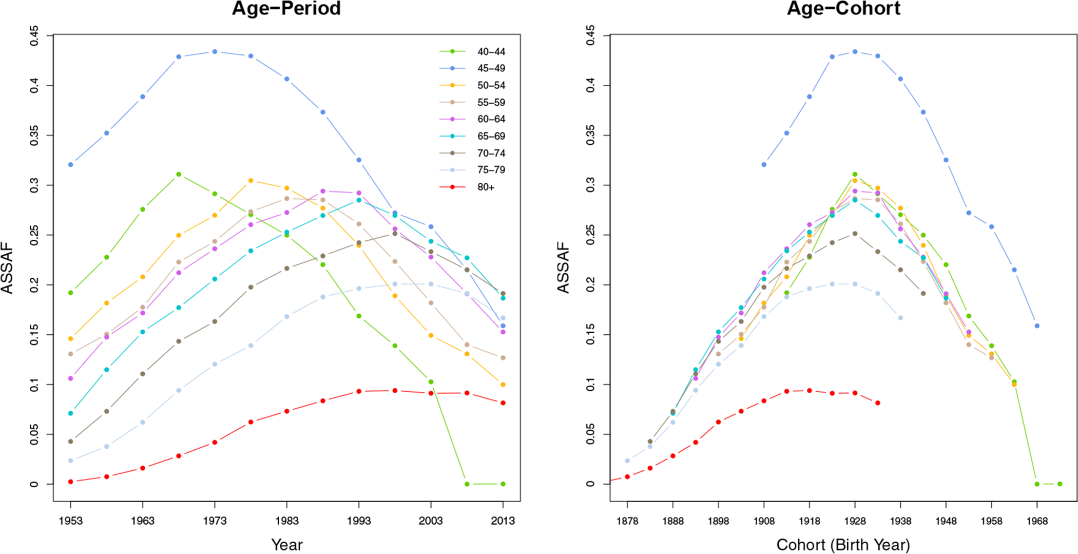
Age-specific smoking attributable fractions (ASSAF) for the male population in the United States from 1950–2015. Left: Age-period plot. The horizontal axis is the year of observation and colors differentiate age groups. Right: Age-cohort plot. The horizontal axis is the year of birth for all cohorts, where the values for each age group are shown by a different color.
2.3.1. Estimation and Forecasting: Age-cohort Modeling
We propose a probabilistic age-cohort approach to estimate and forecast the ASSAF for the male population. The age-cohort plot of the US male ASSAF (right panel) in Figure 1 has two main features that lead to our modeling. First, the ASSAF can be well approximated by the product of an age effect and a cohort effect. The ASSAF of age group 80+ tends to shift horizontally from other age groups for most of the countries (e.g., see the red dashed line in the age-cohort plot of Figure 1 for the case of US males). Hence, we apply a cohort effect τ for all age groups less than 80, and a separate cohort effect for the 80+ age group.
The probabilistic model of ASSAF in country ℓ is
| (1) |
where x takes values in {40, 45, 50, 55, 60, 65, 70, 75, 80}. To ensure identifiability, we set for all countries. Eq. (1) is also closely related to a low-rank matrix completion method. The age-cohort matrix based on the observed period ASSAF inevitably contains missing values since we do not observe the ASSAF of early cohorts at young ages or that of late cohorts at old ages (see Figure 2).
Figure 2:

Transformation from age-period matrix (left) to age-cohort matrix (right). Black and grey cells represent observed and missing values, respectively.
Second, the cohort pattern of the male ASSAF has a strong increasing-peaking-declining pattern. This trend can be well captured by a five-parameter double logistic function (Meyer, 1994):
| (2) |
where θ := (Δ1, Δ2, Δ3, Δ4, k). The double logistic curve is a flexible parametric curve, which has been used in many scientific fields such as hematology, phenology, and agricultural science. Due to its scientific interpretability, it is often used to describe social change, diffusion, and substitution processes (Grübler et al., 1999; Fokas, 2007; Kucharavy and De Guio, 2011). Examples of the use of a double logistic curve to describe dynamics in human demography include mortality rates (Marchetti et al., 1996), life expectancy at birth (Raftery et al., 2013), and total fertility rates (Alkema et al., 2011).
Most developed countries have already entered the declining stage of the smoking epidemic. The epidemic started in the early 1900s with a steady increase until the 1950s-60s when the adverse impact of smoking became widely known and anti-smoking measures started to be put in place. Since then, the smoking epidemic has continued to decline. Thus the cohort effect of smoking exhibits a similar increasing-peaking-decreasing trend, which can be captured naturally by the double logistic curve.
The cohort effect for ages 80+ is just a horizontal shift of the cohort effect τ for younger ages, so we use two related double logistic curves to bridge them:
| (3) |
where c := t − x, , and . Here δℓ is a shift parameter controlling the amount of horizontal translation can make with respect to τ.
We use a three-level Bayesian hierarchical model (BHM) to estimate and forecast male ASSAF for all countries of interest jointly. Level 1 models the observed male ASSAF in terms of the tensor product of the age effect and the cohort effect (i.e., Eq. (1)). Level 2 models the distributions (conditioning on the global parameters) of the country-specific age effect , the country-specific cohort effects and in Eq. (3), the country-specific parameters θℓ and the double logistic function, and the country-specific measurement variance . Level 3 sets hyperpriors on the global parameters
More details of the specification of the full model are given in Appendix A.
The left and right panels of Figure 3 plot the cohort effects and age effect of US male ASSAF, respectively. The estimated cohort effect τ for the age groups 45–79 shows a clear increasing-peaking-decreasing trend as observed in Figure 1. The estimated cohort effect for the 80+ age group shows the same trend for the 13 cohorts reaching age 80 by 2015. We could forecast any cohort effects based on the posterior distribution of the double logistic function. The estimated age effect indicates that the smoking-attributed fraction of mortality is higher among middle-aged males (aged 40–69) in the US than among older males (70 and over). Figure 4 plots the posterior distributions of the means of the US male ASSAF for all 9 age groups and all 21 cohorts.
Figure 3:
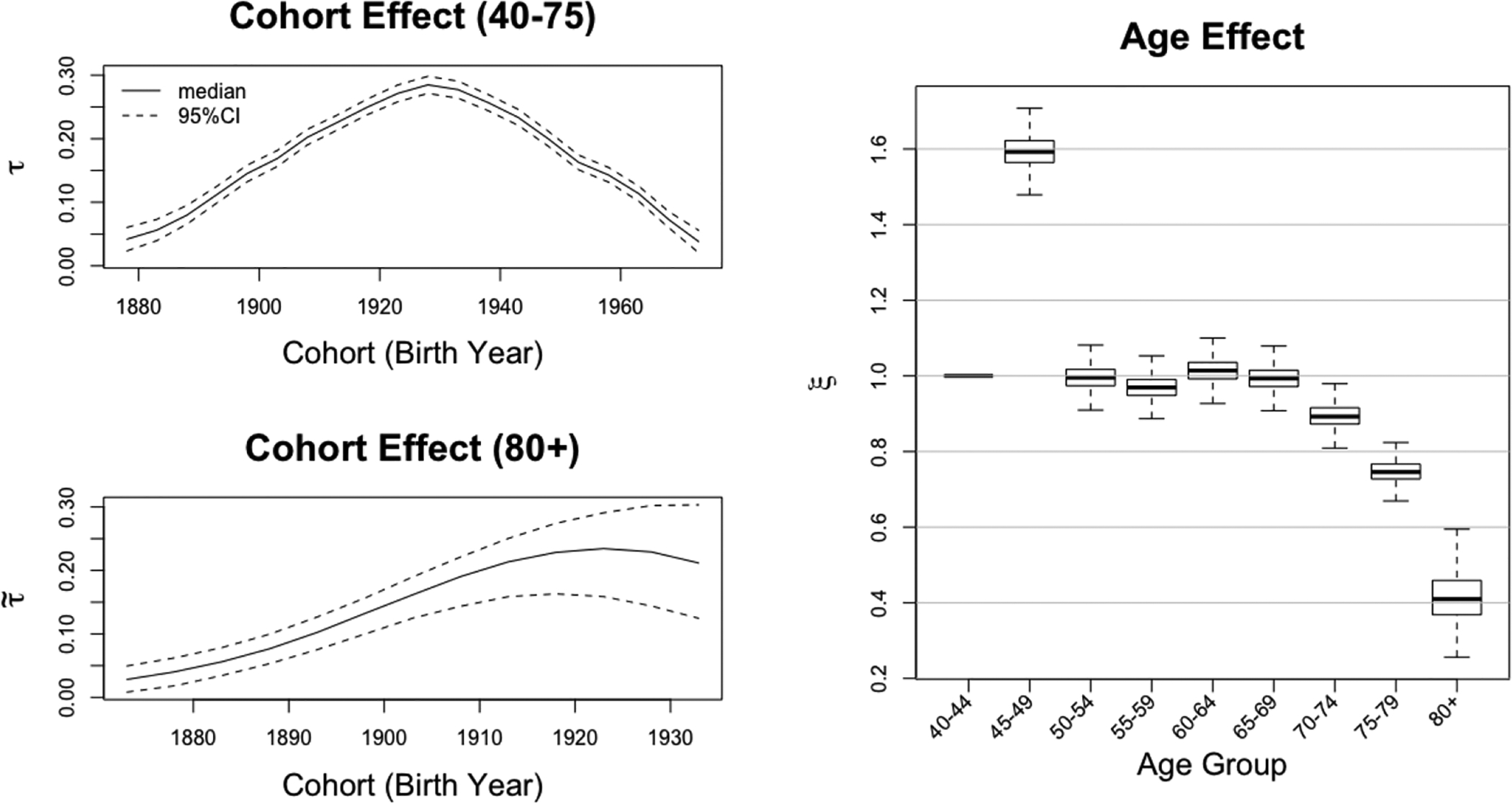
Posterior distributions of cohort and age effects of United States male ASSAF. Top Left: posterior median and 95% credible intervals of the cohort effects τ for the 40–79 age groups. Bottom Left: posterior median and 95% credible intervals of the cohort effect for the 80+ age groups. Right: boxplot of posterior distribution of the age effect.
Figure 4:
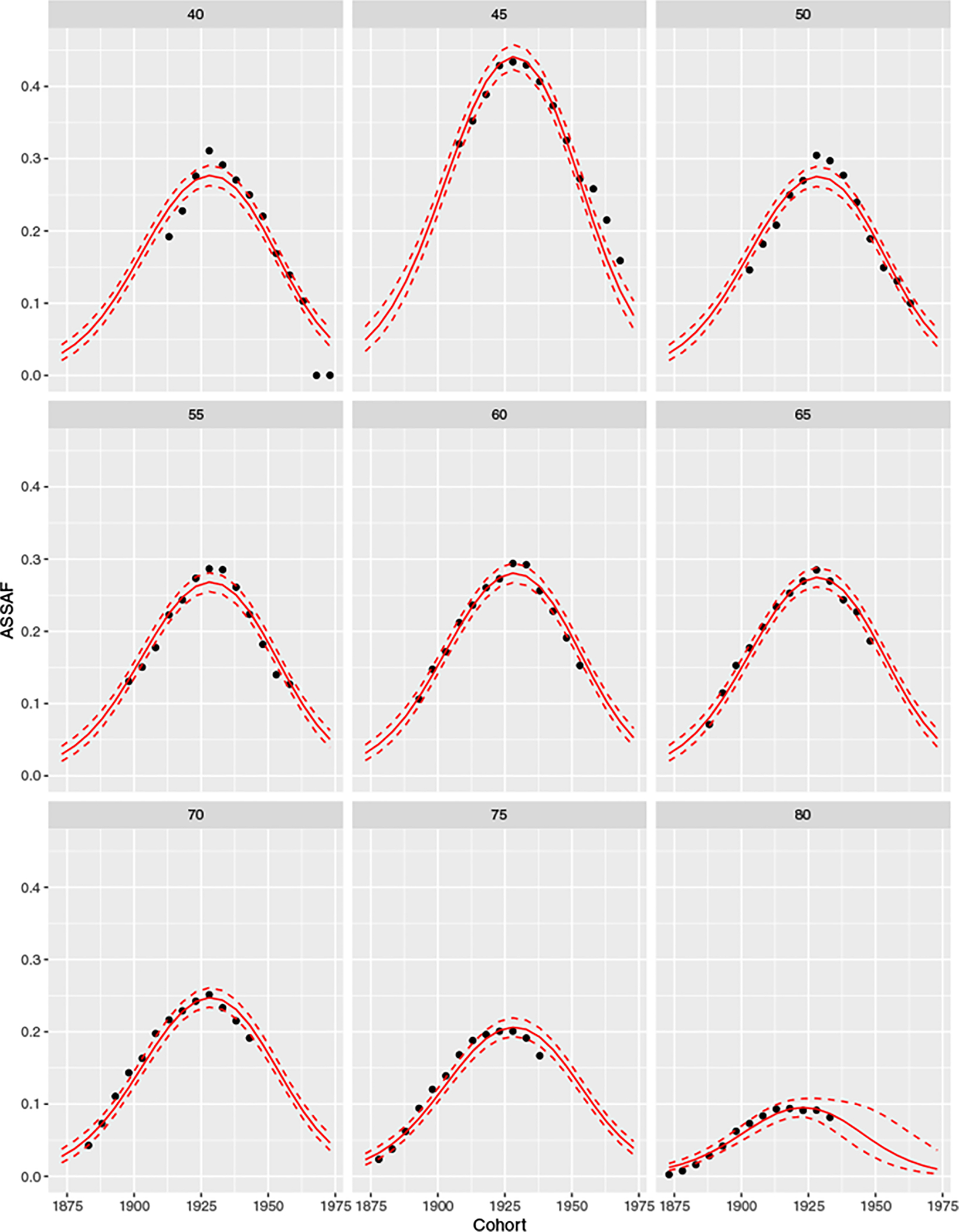
Posterior distributions of the means of US male ASSAF for all 9 age groups. The observed ASSAF is shown by black dots. The posterior median and 95% credible intervals of the means are shown by solid and dashed red lines, respectively.
To project the future ASSAF, we first generate future cohort effects by plugging samples drawn from the posterior distributions of country-specific parameters θℓ and in Eq. (2) and (3). Then, we apply Eq. (1) using samples drawn from posterior distributions of the future cohort effects, age effect, and country-specific variance to get projections of ASSAF.
2.4. Non-smoking Life Expectancy
The non-smoking life expectancy at birth, , is the life expectancy at birth that a population would have if no one smoked, but all mortality risks were otherwise the same (Bongaarts, 2006). To estimate , we need the age-specific mortality rates dx and the ASSAF yx described in Section 2.3. As in the last section, all quantities described in this section are specific to the male population, and the sex index s is omitted unless otherwise specified.
The calculation of consists of two steps. First, the age-specific non-smoking attributable mortality rate for a given country ℓ, age group x, and period t (denoted by ) is calculated as
| (4) |
Second, we convert the set of to using the standard period life table method (Preston et al., 2000, Chapter 3), as implemented in the life.table function in the R package MortCast (Ševčíková et al., 2019a). Figure 5 shows the relationship between quinquennial e0 and for US males and Netherlands males from 1950 to 2015, respectively. The vertical gap between e0 and at each time point presents the years of life expectancy lost due to smoking. The changes in the gaps also follow a similar increasing-peaking-decreasing trend over the period 1950 to 2015.
Figure 5:
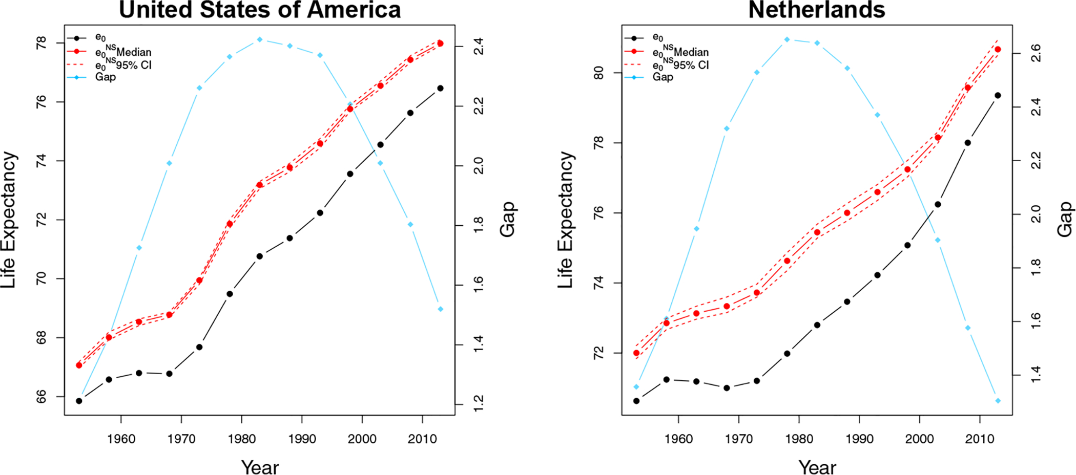
Male life expectancy at birth, e0, and male non-smoking life expectancy at birth, , for the United States (left) and the Netherlands (right). The black line shows e0. The solid red line and the dashed red lines show the posterior median and the 95% credible interval of . The blue line represents the gap between e0 and .
2.4.1. Estimation and Forecasting: Non-linear Life Expectancy Gain Model
We forecast by investigating the nonlinear five-year gains of . As discussed by Raftery et al. (2013), the improvement of gains on e0 for most of the countries has experienced a slow-rapid-slow increasing pattern and a six-parameter double logistic function is used to capture the non-linearity of five-year gains of e0:
| (5) |
where ζ := (a1, a2, a3, a4, w, z) and z is the asymptotic average rate of increase in e0. We assume that z is nonnegative, implying that life expectancy will continue to increase on average (Oeppen and Vaupel, 2002; Bongaarts, 2006).
The five-year gains in exhibit this nonlinear pattern as well. The left panel of Figure 6 plots the observed five-year gains of e0 (in grey dots) and (in red dots) for the 69 countries with data of high enough quality from 1950 to 2015. The five-year gains in have nearly the same shape as the five-year gains in e0, which supports using the same double logistic function to model the gains. Also, has almost the same five-year gain at the highest age as e0, suggesting that the asymptotic average rate of increase z for should be similar to that of e0. Further, the variability of the five-year gains of changes from a low level to a high level of , which suggests including a nonconstant variance component in the model.
Figure 6:
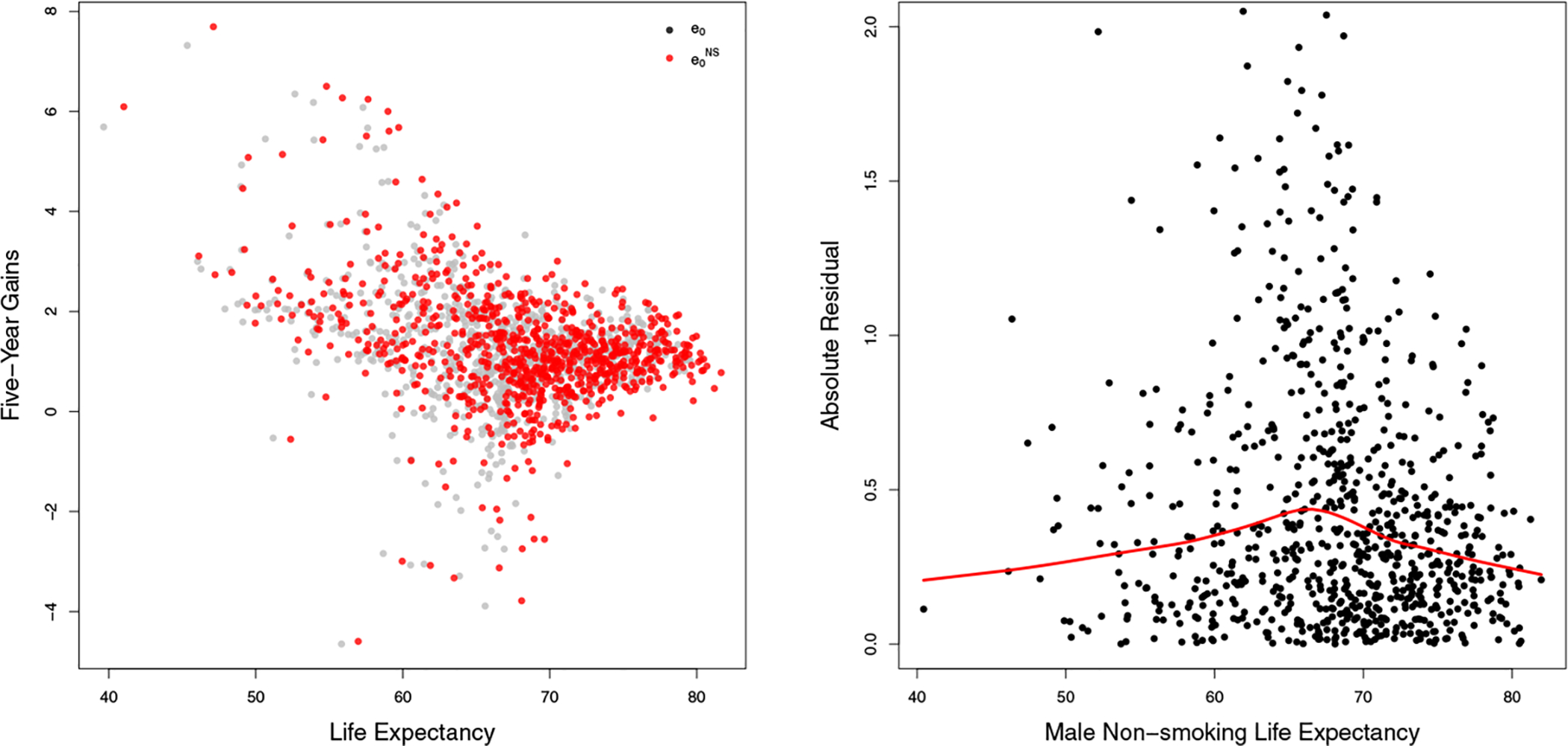
Left: Five-year gains of e0 and for 69 countries from 1950 to 2015. The gains in e0 and are represented using grey and red dots, respectively. Right: Plot of absolute residuals estimated from the constant variance model against life expectancy shown by black dots, with fitted regression spline shown by the red line.
We use a three-level Bayesian hierarchical model for . Level 1 models for country ℓ and period t by
| (6) |
with country-specific parameters . Here ϕ(·) is a regression spline fitted to the absolute residuals resulting from the model with constant variance in Eq. (6) with the same estimation method described later. The regression spline is used to account for the changing variability of the observed data. The right panel of Figure 6 illustrates the varying absolute residuals with the fitted spline in red. Level 2 specifies the conditional distribution for all country-specific parameters including ζℓ and ωℓ. Level 3 sets the hyperpriors for the global parameters . The full specification of the model is given in Appendix A.
To produce a probabilistic forecast, we sample from the joint posterior distributions of the country-specific parameters ζℓ to calculate the five-year gains together with the posterior distributions of ωℓ. For the variance component, we evaluate if is within the range of the fitted data; otherwise, it is set equal to the spline value evaluated at the largest observed . We then use Eq. (5) and (6) to generate samples from the posterior predictive distribution for future country-specific . The set of samples approximates the posterior predictive distribution.
2.5. Male-Female Joint Forecast
2.5.1. Male e0 Forecast
First, we use the coherent Lee-Carter method (Li and Lee, 2005; Ševčíková et al., 2016) to convert the projected back to for all age groups x at period t of country ℓ. Then, we invert Eq. (4) to get the projected age-specific all-cause mortality,
for any age groups x, period t, and country ℓ. Finally, applying the same life table method described in Section 2.4 to the forecast , we obtain the forecast life expectancy at birth for period t and country ℓ. Figure 7 illustrates the projections of and e0 for US and the Netherlands males to 2060. The projected e0 converges to the projected as ASSAF decreases towards 0 for all age groups of US and the Netherlands males.
Figure 7:
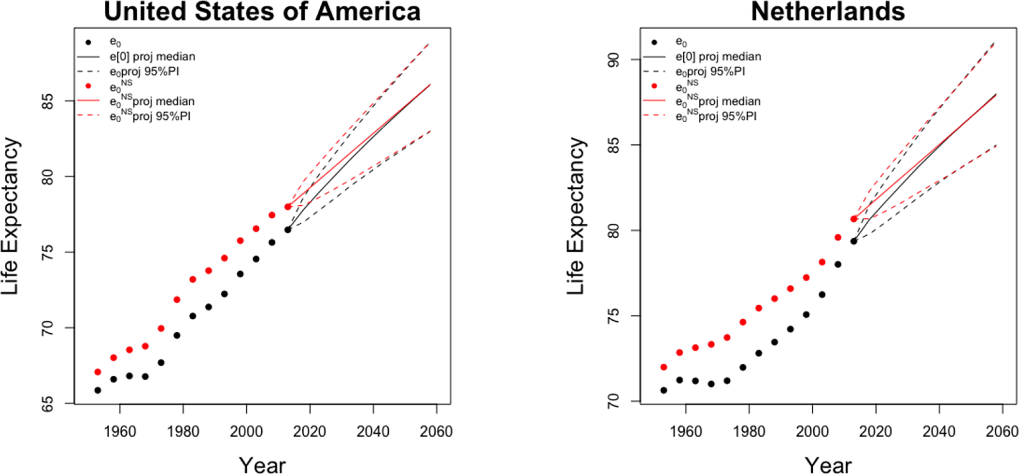
Projections of and e0 of US (left) and the Netherlands (right) males to 2060. The posterior medians and the 95% predictive intervals of projected are shown by solid and dashed red lines, respectively. The posterior medians and the 95% predictive intervals of projected e0 are shown by solid and dashed black lines, respectively.
2.5.2. Female e0 Forecast: Gap Model
We propose a gap model similar to that of Raftery et al. (2014b) to produce a coherent projection of male-female life expectancy at birth. It has been argued that differences in smoking largely account for the life expectancy gap between males and females (Preston and Wang, 2006; Wang and Preston, 2009). Here we explore the relationship between the between-sex gap in life expectancy and the between-sex gap in the all-age smoking attributable fraction (ASAF). The ASAF is a single statistic summarizing the smoking effect on mortality and is defined as a weighted average of the ASSAF values as calculated in Section 2.3, where the weights are the age-specific mortality rates. Li and Raftery (2019) describe the estimation of ASAF, as well as a method for forecasting it using a four-level Bayesian hierarchical model.
We modify the gap model of Raftery et al. (2014b) by adding the country-specific between-sex ASAF gap as a covariate. The proposed gap model is as follows:
| (7) |
where U and L are the observed historical maximum and minimum of the between-sex gap in e0, ϖ is the level of male e0 at which the gap is expected to stop widening, and ht is the between-sex gap (male minus female) of the posterior median of ASAF in period t.
The estimated parameters of the model based on the data for 69 countries for 1950–2015 are reported in Table 1. Our estimates indicate that the e0 sex gap has a strong positive association with the ASAF gap after adjusting for other factors ( with p-value < 10−5). Since the estimated lower bound of the life expectancy gap L is positive, our model guarantees that no crossover of male and female life expectancy forecasts will happen for all trajectories. The other coefficients have similar estimates and significance as in Raftery et al. (2014b), which accounts for the remaining variability in the between-sex life expectancy gap, possibly due to biological and other social factors (Janssen and van Poppel, 2015).
Table 1:
Estimated gap model coefficients with standard errors in parentheses, if available.
| Variable | Parameter | Estimate | Variable | Parameter | Estimate |
|---|---|---|---|---|---|
| Intercept | β0 | −1.965 (0.629) | β5 | 1.183 (0.284) | |
| β1 | 0.010 (0.003) | σG | 0.494 | ||
| β2 | 0.896 (0.010) | ϖ | 61 | ||
| β3 | 0.041 (0.011) | L | 0.03 | ||
| β4 | −0.102 (0.012) | U | 13.35 | ||
| R2 | 0.934 | ||||
When performing projection, we forecast all terms in Eq. (7) forward. Instead of using a random walk as in Raftery et al. (2014b), we make use of the ASAF gap to guide our projection. However, we constrain the quantity to be 20 when is greater than 81 years, which is the largest male e0 observed in countries of interest up to 2015, since there is not enough information to determine whether the gap will continue to shrink for higher e0. After the gender gap has been forecast, we add the gap to each posterior trajectory of the forecast male e0 to get the full posterior predictive distribution of female e0.
2.6. Estimation and Projection of the Full Model
We use data from 69 countries for which the data on the male smoking-attributable mortality was of good enough quality. The precise data quality criteria and thresholds used are described in Li and Raftery (2019). Of these 69 countries, two are in Africa, 16 are in the Americas, nine are in Asia, 40 are in Europe and two in Oceania. Estimation of the full model makes uses of male ASSAF, male age-specific mortality rates, both sexes e0, and both sexes ASAF of all 69 clear-pattern countries over 13 five-year periods during 1950–2015. Future e0 of the same set of countries over 9 five-year periods from 2015 to 2060 is projected based on the joint posterior predictive distribution of the full model. The full procedure is described in Appendix A.
We use Markov Chain Monte Carlo (MCMC) to sample from the joint posterior distributions of the parameters of interest. For the BHM of the ASSAF, we ran three chains, each of length 100,000 iterations thinned by 20 iterations with a burn-in of 2,000. This yielded a final, approximately independent sample of size 3,000 for each chain. For the BHM of each of the 30 samples of , we ran one chain with length 100,000 iterations thinned by 50 with a burn-in of 1,000. This yielded a final, approximately independent sample of size 1,000 for each chain. We monitored convergence by inspecting trace plots and using standard convergence diagnostics, details of which are given in Appendix B. We include the plots of e0 projections for all 69 countries and both sexes in Appendix C.
3. Results
We assess the predictive performance of our model using out-of-sample predictive validation.
3.1. Study design
The data we used for out-of-sample validation cover the period 1950–2015, dividing it into an earlier training period and a later test period. We fit the model using only data from the training period, and then generated probabilistic forecasts for the training period. We finally compared the probabilistic forecasts with the observations for the training period. We used two different choices of test period: 2000–2015, and 2010–2015. The former allows us to assess longer-term forecasts, while the latter focuses on shorter-term forecasts.
To assess the accuracy of the probabilistic forecasts, we define the sex-specific mean absolute error (MAE) as
| (8) |
where is the set of countries considered in the validation, is the set of training periods, and is the posterior median of the predictive distribution of life expectancy at birth at year t for country ℓ and sex s. To assess the calibration and sharpness of the model, we calculated the average empirical coverage of the prediction interval over the validation period, which we hope to be close to its nominal level with as short a halfwidth of the interval as possible (Gneiting and Raftery, 2007).
3.2. Out-of-sample validation
We evaluated and compared the performance of the proposed model with four commonly used methods for forecasting e0: the Lee-Carter method (Lee and Carter, 1992), the Lee-Miller method (Lee and Miller, 2001), the Hyndmann-Ullah functional data method (Hyndman and Ullah, 2007), and the Bayesian hierarchical model as implemented in the bayesLife R package (Raftery et al., 2013). We refer to the last as the bayesLife method. The first three methods were implemented using the corresponding functions with default settings in the demography R package (Booth et al., 2006; Hyndman et al., 2019). The bayesLife method was implemented under default settings using the R package bayesLife (Raftery et al., 2013, 2014b; Ševčíková et al., 2019b).
Table 2 gives the out-of-sample validation results for the four methods described above as well as our proposed method. Our method had the smallest MAE for both sexes and both choices of test period among the five methods. For predicting one five-year period ahead, our method improved accuracy over the Lee-Carter method by 70% (67%), and over the bayesLife method by 24% (28%) for males (females). For predicting three five-year periods ahead, the new method improved accuracy over the Lee-Carter method by 53% (40%), and over the bayesLife method by 24% (17%) for males (females).
Table 2:
Out-of-sample validation results for forecasting life expectancy at birth of males and females one and three five-year periods ahead. “Num” is the number of countries used in the validation. In the “Method” column, “H-U FDA” is the Hyndman-Ullah functional data analysis method, “bayesLife” represents the method described in Raftery et al. (2013), and “smokeLife” is the our proposed method. “Halfwidth” represents the median of the halfwidth of the prediction interval.
| Period | Num | Sex | Method | MAE | Coverage | Halfwidth | ||
|---|---|---|---|---|---|---|---|---|
| 80% | 95% | 80% | 95% | |||||
| Train:1950–2000 | 67 | M | Lee-Carter | 2.043 | 0.144 | 0.199 | 0.368 | 0.568 |
| Lee-Miller | 1.536 | 0.318 | 0.418 | 0.831 | 1.239 | |||
| H-U FDA | 2.206 | 0.189 | 0.274 | 0.808 | 1.259 | |||
| bayesLife | 1.273 | 0.741 | 0.950 | 1.722 | 2.714 | |||
| smokeLife | 0.962 | 0.741 | 0.896 | 1.197 | 1.943 | |||
| Test: 2000–2015 | F | Lee-Carter | 1.210 | 0.199 | 0.294 | 0.391 | 0.599 | |
| Lee-Miller | 0.748 | 0.602 | 0.756 | 0.612 | 0.940 | |||
| H-U FDA | 1.430 | 0.114 | 0.299 | 0.412 | 0.633 | |||
| bayesLife | 0.876 | 0.816 | 0.955 | 1.312 | 1.985 | |||
| smokeLife | 0.728 | 0.876 | 0.985 | 1.373 | 2.166 | |||
| Train:1950–2010 | 68 | M | Lee-Carter | 1.741 | 0.103 | 0.118 | 0.306 | 0.448 |
| Lee-Miller | 0.853 | 0.544 | 0.721 | 0.581 | 0.931 | |||
| H-U FDA | 1.364 | 0.191 | 0.324 | 0.548 | 0.791 | |||
| bayesLife | 0.688 | 0.824 | 0.897 | 1.098 | 1.748 | |||
| smokeLife | 0.523 | 0.912 | 0.985 | 0.773 | 1.250 | |||
| Test: 2010–2015 | F | Lee-Carter | 1.025 | 0.118 | 0.221 | 0.279 | 0.436 | |
| Lee-Miller | 0.486 | 0.662 | 0.779 | 0.476 | 0.708 | |||
| H-U FDA | 0.895 | 0.250 | 0.368 | 0.373 | 0.573 | |||
| bayesLife | 0.464 | 0.868 | 0.941 | 0.853 | 1.291 | |||
| smokeLife | 0.319 | 1.000 | 1.000 | 0.970 | 1.509 | |||
For model calibration, the Lee-Carter-type models produced predictive intervals that are too narrow, thus underestimating the predictive uncertainty in the testing period. The bayesLife method and the new method produced predictive intervals with coverage close to the nominal level. We assess the sharpness of the forecast method using the 80% predictive interval halfwidth. For male data under the three five-year periods prediction, the 80% predictive interval of the new method was 30% shorter on average, but yielded the same empirical coverage as the bayesLife method. Under the one five-year out-of-sample predictions, the 80% predictive interval of the new method was 30% shorter on average but yielded even higher empirical coverage than the bayesLife method. For female data, the predictive intervals of our method overcovered the observations slightly for each choice of test period, but their median halfwidths were not much wider than those of the bayesLife method (e.g., the largest increment was less than 18%). The major source of variability in the female projections of the new method comes from the gap model.
4. Case studies
On average, smoking results in 1.4 years lost of male life expectancy at birth for the 69 countries over 1950–2015. The trend in years lost due to smoking also follows the pattern of the smoking epidemic. The average years lost due to smoking among males increased from 0.9 in 1953 to a maximum of 1.7 in 1993, and decreased to 1.3 in 2013.
For male populations of most countries, the ASSAF has already passed the peak for most age groups. When this is the case, accounting for the smoking effect leads to higher forecasts of life expectancy at birth. On average, our proposed method gives forecasts of male life expectancy at birth that are 1.1 years higher than the bayesLife method used by the UN for the 69 countries over the period 2015–2060.
Most female populations are still at the increasing or peaking stage of the smoking epidemic. However, for 2055–2060, we expect to see an increment of 1.07 in female life expectancy, since the female smoking epidemic will be following the same decreasing trend as that of males by then.
We now study four countries in detail, representing different patterns of the smoking epidemic.
4.1. United States
The United States of America has one of the best vital registration systems in the world and also high quality data on cause of death. It thus has high quality data on the SAF. The smoking epidemic started in the early 1900s among the male population and rose to the historical maximum of around 60% in the 1950s. At that point, government programs and social movements against smoking began to develop, and the US public became increasingly aware of the adverse impacts of smoking. Since then, there has been a substantial decrease in smoking prevalence, going down to about 20% in the 1990s, and 17.5% in 2016 (Burns et al., 1997; Islami et al., 2015).
The female smoking epidemic started two decades later than the male one with a maximum prevalence of around 30% in the 1960s. Female smoking prevalence decline to about 20% in 1990s and 13.5% in 2016 (Burns et al., 1997; Islami et al., 2015). Figure 8a shows projections of the US male and female ASAF to 2060. Figure 8b predicts a continuously narrowing gap of the between-sex life expectancy due to the shrinking gap between male and female ASAF up to 2060.
Figure 8:
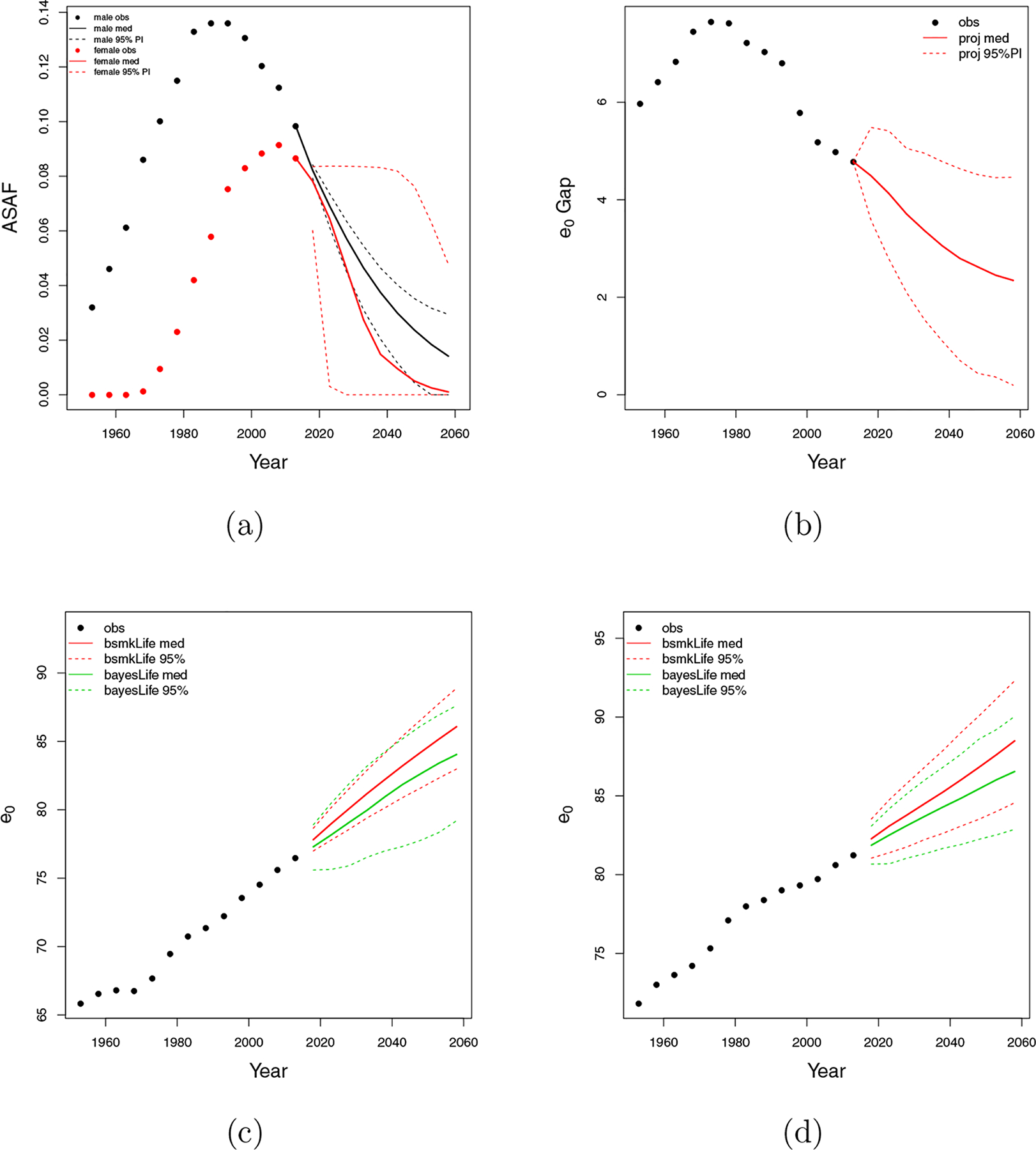
United States of America. (a) All-age smoking attributable fraction (ASAF) for male (black) and female (red) with median and 95% PI of posterior predictive distributions. (b) Between-sex gap of life expectancy at birth with posterior predictive median (red solid) and 95% PI (red dotted). (c) Forecasts of male life expectancy at birth to 2060 using bayesLife method (green) and our proposed method (red) with posterior predictive medians (dashed) and 95% PI (dotted). (d) Forecasts of female life expectancy at birth to 2060 using bayesLife method (green) and our proposed method (red) with posterior predictive medians (dashed) and 95% PI (dotted).
Figures 8c and 8d show projections of male and female life expectancy for the period 2015–2060. The bayesLife method projects male life expectancy in 2055–2060 to be 84.0 years, with 95% predictive interval (79.2, 87.6). We project male life expectancy to be 86.1 in 2060, with 95% predictive interval (83.0, 88.9). The bayesLife method projects US female life expectancy for 2055–2060 to be 86.5 with 95% predictive interval (82.9, 90.0). We project female life expectancy to be 88.5 with interval (84.6, 92.3).
Our method gives forecasts of life expectancy that are about two years higher than those from the bayesLife method for both males and females, because of accounting for the smoking effect. Our predictive interval for male life expectancy at birth is 29% shorter than the bayesLife one, while our female interval is comparable with that of the bayesLife method. Both of our 95% predictive intervals cover the posterior medians from the bayesLife method.
4.2. The Netherlands
The Netherlands is a western European country with a long history of the smoking epidemic, which can be dated back to the 1880s when the cigarette industry began there. Male smoking prevalence reached 90% in most age groups in the 1950s, but dropped rapidly to 30% in the 2010s. In contrast, smoking was more prevalent among females in the 1970s, when about 40% of female smoked, and after 1975 there was a sustained drop to 24% in the 2010s (Stoeldraijer et al., 2015).
Figure 9a shows that the female ASAF is forecast to surpass the male ASAF for the next two decades and by 2060, both male and female ASAF will be at about the same level. Figure 9b shows that the turning point in the between-sex gap of life expectancy happened around the 1990s, when the male ASAF had passed its peak and the female ASAF started to climb. With the shrinking of the ASAF gap, the projected life expectancy gap is forecast to continue to shrink and plateau around 2.5, due to biological and social factors (Janssen and van Poppel, 2015).
Figure 9:
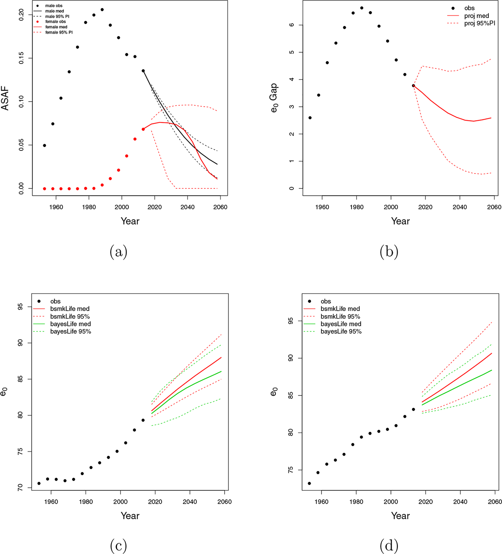
The Netherlands. (a) All-age smoking attributable fraction (ASAF) for male (black) and female (red) with median and 95% PI of posterior predictive distributions. (b) Between-sex gap of life expectancy at birth with posterior predictive median (red solid) and 95% PI (red dotted). (c) Forecasts of male life expectancy at birth to 2060 using bayesLife method (green) and our proposed method (red) with posterior predictive medians (dashed) and 95% PI (dotted). (d) Forecasts of female life expectancy at birth to 2060 using bayesLife method (green) and our proposed method (red) with posterior predictive medians (dashed) and 95% PI (dotted).
Both Dutch males and females experienced a period of stagnation in life expectancy gains—in the 1960s for males and the 1990s for females. Smoking is a major reason for this stagnation. The right panel of Figure 5 indicates that the forecast Dutch male life expectancy gain is more linear and sustained after removing the smoking effect. Figures 9c and 9d show projections of male and female life expectancy for 2015–2060. We project male life expectancy for the period 2055–2060 to be 88.0 years, with a 95% prediction interval of (85.0, 91.1), while the bayesLife method projects 86.1, with interval of (82.3, 89.7). We project female life expectancy for the period 2055–2060 to be 90.6, with a 95% prediction interval of (86.6, 94.8), while the bayesLife method projects 88.4 years, with interval of (85.1, 91.9).
Similarly to the US, our forecast of life expectancy in 2060 is about two years higher than a forecast that does not take account of smoking. By considering the decreasing trend of the smoking epidemic, our forecast is 1.9 years higher for males and 2.3 years higher for females expectancy compared with the bayesLife method. Janssen et al. (2013) forecast the Dutch male and female life expectancy in 2040 to be 84.6 years and 87.2 years respectively, taking account of smoking. This agrees well with our forecasts —85.0 for males and 87.4 for female—in 2040.
4.3. Chile
Chile is a South American country where the smoking epidemic had a late start, and it is currently one of the countries with the highest smoking prevalence in the Americas. Smoking prevalence decreased from 50% in 2000 to 40% in 2016 among males, and from 44% to 36% among females. This decline is modest compared to that in the United States (Islami et al., 2015).
Figure 10a shows the projections of male and female ASAF. Chilean male ASAF has been at the peaking stage for a long time, with high prevalence and no sign of a decline. Female ASAF is predicted to grow to approach the male level. The narrowing of the ASAF gap is forecast to lead to a sustained closing of the life expectancy between-sex gap (Figure 10b).
Figure 10:
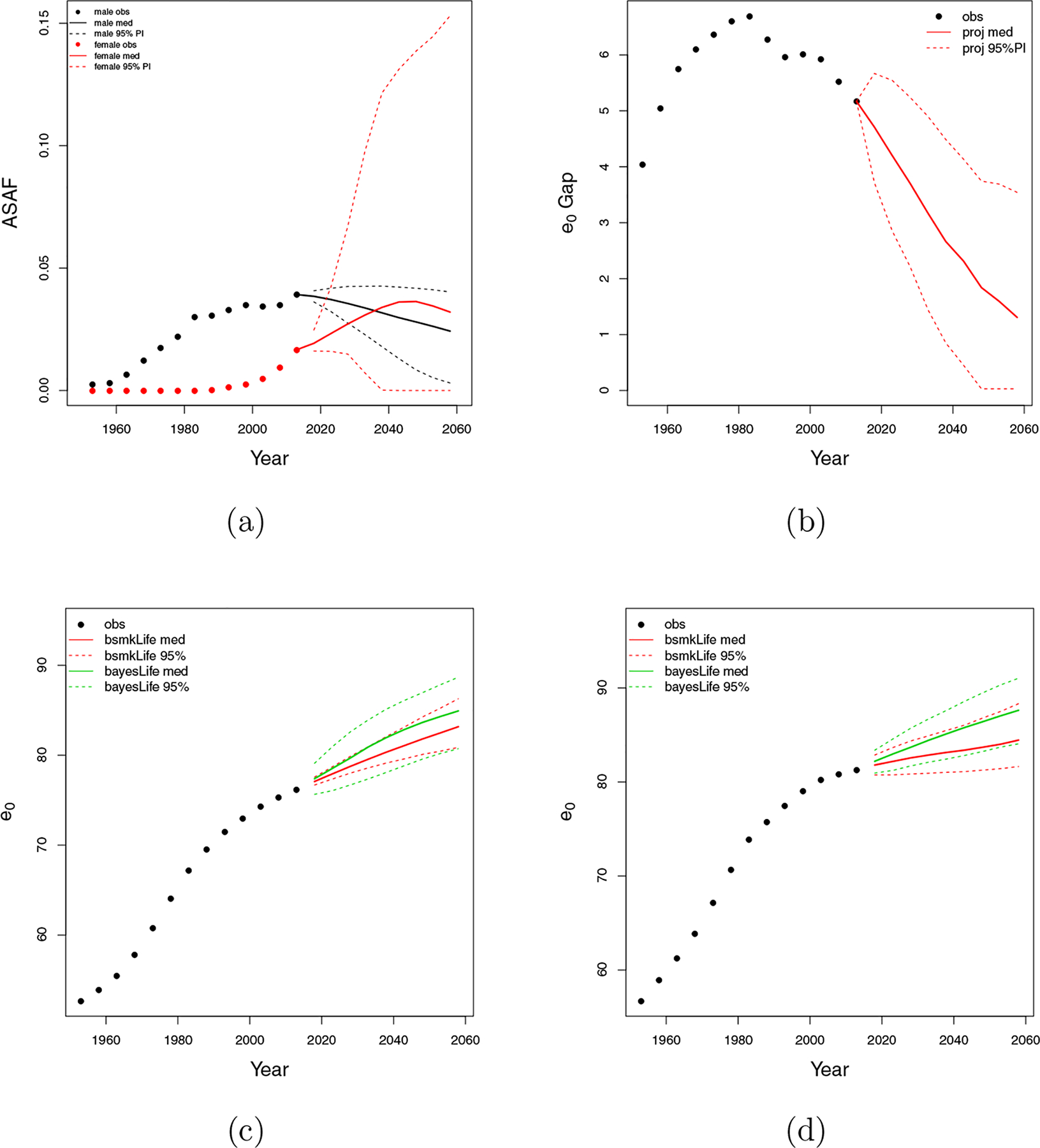
Chile. (a) All-age smoking attributable fraction (ASAF) for male (black) and female (red) with median and 95% PI of posterior predictive distributions. (b) Between-sex gap of life expectancy at birth with posterior predictive median (red solid) and 95% PI (red dotted). (c) Forecasts of male life expectancy at birth to 2060 using bayesLife method (green) and our proposed method (red) with posterior predictive medians (dashed) and 95% PI (dotted). (d) Forecasts of female life expectancy at birth to 2060 using bayesLife method (green) and our proposed method (red) with posterior predictive medians (dashed) and 95% PI (dotted).
Figures 10c and 10d show projections of male and female life expectancy for 2015–2060. We project male life expectancy for the period 2055–2060 be 83.2, with a 95% predictive interval of (80.9, 86.3). In contrast with the USA and the Netherlands, our median projection is 1.8 years less than that from bayesLife method. This is due to the fact that the epidemic has not yet clearly peaked. We project female life expectancy to be 84.5, with a 95% predictive interval of (81.6, 88.3), which is again substantially smaller than that from the bayesLife method with forecast median 87.6 years and 95% prediction interval (84.1, 91.0). This is due to the increasing impact of smoking on the Chilean female population.
4.4. Japan
Japan has been a leading country in life expectancy for a long period, while it also has a long history of smoking and is one of the largest tobacco consumers. Male smoking prevalence reached 83.7% in 1966. That number dropped to 36% in the 1990s and halved again by 2018. Female smoking prevalence is far lower and changes less dramatically than that of males. Female smoking prevalence reached 16% in the 1970s and decreased to 9.7% in 2015. The significant changes result mainly from government regulations and anti-smoking movements starting in the 1980s. Figure 11a shows the forecast male and female ASAF. Figure 11b shows the narrowing of the life expectancy gap as a result.
Figure 11:
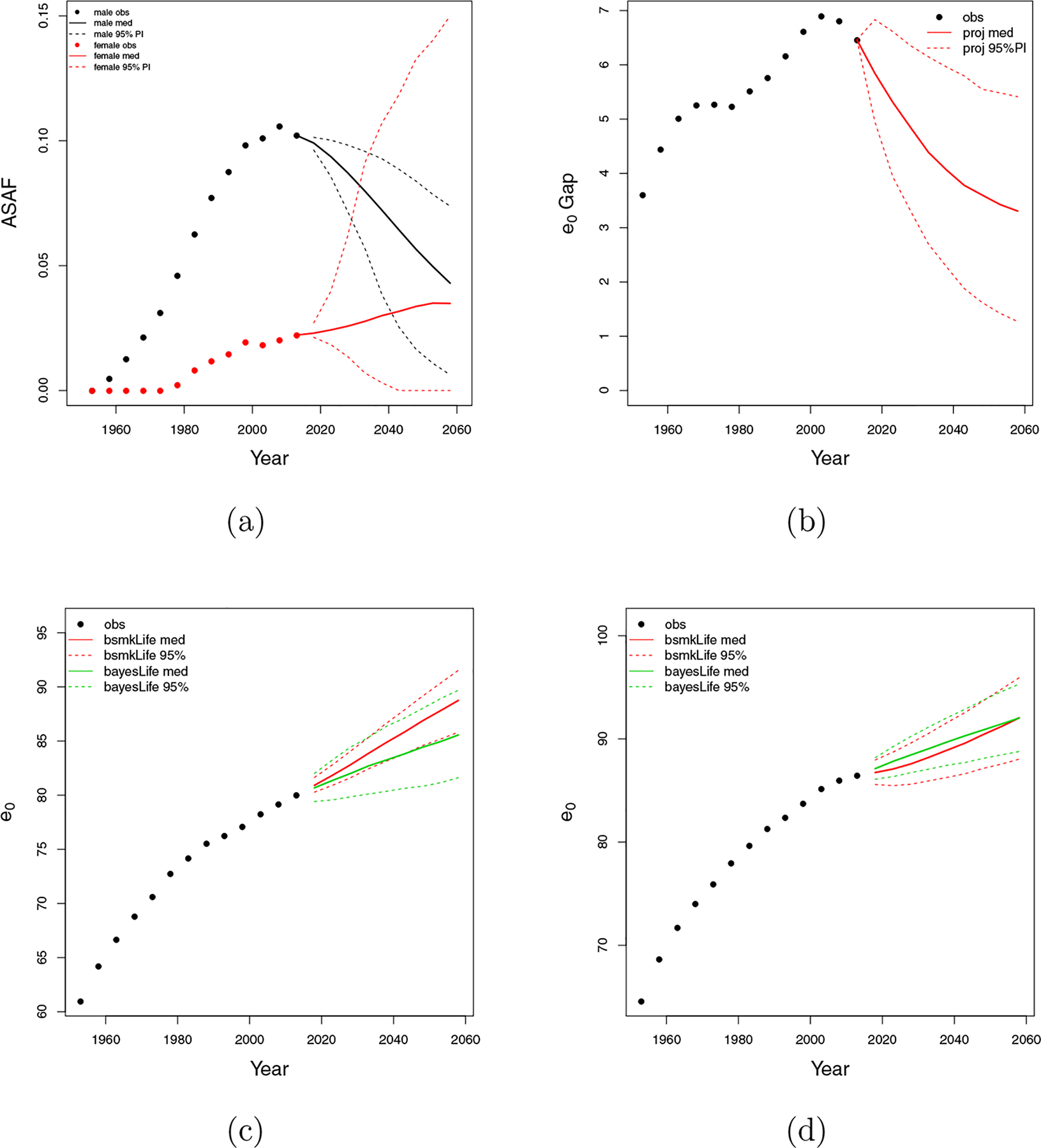
Japan. (a) All-age smoking attributable fraction (ASAF) for male (black) and female (red) with median and 95% PI of posterior predictive distributions. (b) Between-sex gap of life expectancy at birth with posterior predictive median (red solid) and 95% PI (red dotted). (c) Forecasts of male life expectancy at birth to 2060 using bayesLife method (green) and our proposed method (red) with posterior predictive medians (dashed) and 95% PI (dotted). (d) Forecasts of female life expectancy at birth to 2060 using bayesLife method (green) and our proposed method (red) with posterior predictive medians (dashed) and 95% PI (dotted).
Figures 11c and 11d show projections of life expectancy for males and females. We project male life expectancy for the period 2055–2060 to be 88.8, with a 95% predictive interval of (85.8, 91.5). The bayesLife method forecasts 85.6, with a projection interval (81.6, 89.7). Notice that our median forecast is 3.2 years higher than that of bayesLife, while its interval is 1.4 years narrower. We project female life expectancy to be 92.0 with a 95% prediction interval of (88.0, 95.9). Our forecast shows a noticeable slowdown of the growth of female life expectancy due to the smoking effect. The bayesLife method projects 92.0 years with interval (88.8, 95.3). Though both methods produce comparable forecast results for 2055–2060, the bayesLife method forecasts a more linear increase while ours reflects the nonlinear smoking effect on the life expectancy forecast.
5. Discussion
We have proposed a method for probabilistic forecasting of mortality and life expectancy that takes account of the smoking epidemic. The method is based on the idea of the smoking attributable fraction of mortality, as estimated by the Peto-Lopez method using data on lung cancer mortality. The age-specific smoking attiributable fraction (ASSAF) of mortality is estimated and used to infer the non-smoking life expectancy at birth, . Both the ASSAF and are then forecast using a Bayesian hierarchical models for all countries with sufficiently good data. This in turn yields posterior predictive distributions of mortality rates and life expectancy at birth. The method performed well in an out-of-sample validation study.
The strength of the method derives from the fact that the smoking attributable fraction of mortality follows a very strong increasing-peaking-decreasing trend over time in all countries where the smoking epidemic has been going for long enough. This pattern is strong, broadly the same across countries, is to a large extent socially determined, and is also not highly correlated over time with the life expectancy at birth itself, which follows a broadly increasing pattern over time. However, smoking does impact mortality. Thus smoking mortality can be predicted with considerable accuracy, and accurate predictions improve mortality forecasts.
Another strength of the method is its use of a hierarchical model, which greatly facilitates forecasting, particularly for countries where the smoking epidemic is at an early stage. This allows forecasts for such countries to be informed by information from other countries, especially those where the epidemic is more advanced. It also makes it easier to incorporate all major sources of uncertainty.
The results indicate that for country-sex combinations where the smoking epidemic is advanced enough that we can expect it to be declining by 2060, incorporating smoking increases forecasts of life expectancy by about two years. When the epidemic is at an earlier stage, though, incorporating smoking tends to reduce forecasts of life expectancy. The results also indicate that much of change over time in the female-male gap in life expectancy is due to relative changes in smoking related mortality.
The biggest limitation of our method is that it relies on the availability of high-quality data on cause of death, particularly lung cancer, which are available for only 69 countries of the 201 or so countries in the world. Thus the biggest improvement in the method would come from improvements in data quality. In particular, China and India are missing from our study, because national data on cause of death of high enough quality are not available. Producing such data should be a focus of future data collection and research. This is very important because, not only are China and India the two most populous countries in the world, but they also have high smoking rates and are likely to experience high smoking mortality in the coming decades.
Several other approaches to the problem have been proposed. Bongaarts (2006) introduced the concept of non-smoking life expectancy, and proposed modeling it in a linear way. However, the time evolution of non-smoking life expectancy appears generally to follow a nonlinear pattern, with gains that broadly follow a non-monotonic increasing-peaking-declining patter. This is modeled in our method by a random walk with a the double logistic drift.
Janssen et al. (2013) proposed directly modeling the ASSAF and the age-specific non-smoking attributable mortality rates. They observed that non-smoking mortality rates decline more linearly than overall mortality rates, making the data fit a Lee-Carter model better. They conducted an age-period-cohort analysis, while we found an age-cohort model to be sufficient. There are well-known identifiability issues with age-period-cohort analysis that our approach avoids. They used a coherent Lee-Carter method. This assumes linear progress in log mortality rates, while in fact progress tends to be nonlinear, and also tends to be more linear on the scale of life expectancy than of log mortality rates, which our double logistic random walk attempts to represent.
The mortality component of the UN’s population projections for all countries is based on the Bayesian hierarchical model of Raftery et al. (2013), which does not take account of smoking. We have shown that this could be improved significantly by taking account of smoking. However, the data to do this are available for only 69 countries currently, and the UN aims to use a unified approach for all the 230 countries and territories that they analyze. Thus extending the UN’s method to take account of smoking in this way might not be feasible in the short term. To do this would likely require a major improvement in data availability for many countries. However, it could be useful for national population and mortality projections for individual countries, for example for planning health services, and also for the private sector, for example for actuarial and insurance analyses.
Acknowledgments
Yicheng Li is Graduate Research Assistant and Adrian E. Raftery is Boeing International Professor of Statistics and Sociology, both at the Department of Statistics, Box 354322, University of Washington, Seattle, WA 98195-4322. This research was supported by NIH grants R01 HD054511 and R01 HD070936, and by the Center for Advanced Research in the Behavioral Sciences at Stanford University. The authors are grateful to John Bongaarts for helpful discussions.
Appendices
A. Full Model Specification
In this Appendix, we first describe the estimating and projection of the full model.
Estimate and forecast the male ASSAF using the 3-level Bayesian hierarchical model described in Section 2.3, and generate 30 samples from the posterior distributions of the mean of ASSAF of all 69 clear-pattern countries for all 13 five-year estimation periods and all 9 five-year periods forecast period;
For each country, generate 30 samples of male based on the ASSAF samples drawn in Step 2 for all 13 five-year estimation periods, and for each of the 30 samples, forecast male of all 69 countries for all 9 five-year periods using the 3-level Bayesian hierarchical model described in Section 2.4;
For each country, forecast male e0 based on the method described in Section 2.5.1 for each of the 30 samples, and combine trajectories from all 30 samples to get the full posterior predictive distribution of male e0;
For each country, apply the gap model described in Section 2.5.2 to the combined trajectories of male e0 to get the full posterior predictive distribution of female e0.
The Bayesian hierarchical model for modeling age-specific smoking attributable fraction (ASSAF) described in Section 2.3 is specified as follows.
where , and
The Bayesian hierarchical model for modeling non-smoking life expectancy described in Section 2.4 is specified as follows.
where ζ := (a1, a2, a3, a4, w, z) and
B. MCMC Diagnostics
We check the convergence of BHM for ASSAF based on trace plots and diagnostics (Raftery and Lewis, 1992) for the global parameters in Level 3. We check one chain with 2,000 burn in iterations and 100,000 samples, with a thinning period of 20 iterations. Table 3 shows the summary statistics of the diagnostics. Figure 12 shows the trace plots of all 3,000 samples of the global parameters.
We do the same for . We check one of the 30 samples with 1,000 burn in iterations, 100,000 samples and a thinning period of 50 iterations. Table 4 shows the summarizing statistics of the diagnostics. Figure 13 shows the trace plots of all 1,000 samples of the global parameters.
Table 3:
Diagnostic statistics for global parameters in BHM for ASSAF. Burn1, Size1, and DF1 are the length of burn-in, required sample size, and dependence factor of the Raftery-Lewis diagnostics with parameters q = 0.025, r = 0.0125, and s = 0.95. Burn2, Size2, and DF2 are the same, but for q = 0.975.
| Parameters | Burn1 | Size1 | DF1 | Burn2 | Size2 | DF2 |
|---|---|---|---|---|---|---|
| - | - | - | - | - | - | |
| 2 | 606 | 1.01 | 2 | 631 | 1.05 | |
| 2 | 641 | 1.07 | 2 | 581 | 0.97 | |
| 2 | 577 | 0.96 | 2 | 631 | 1.05 | |
| 2 | 616 | 1.03 | 2 | 591 | 0.98 | |
| 2 | 601 | 1.00 | 2 | 621 | 1.03 | |
| 2 | 616 | 1.03 | 2 | 621 | 1.03 | |
| 2 | 587 | 0.98 | 2 | 611 | 1.02 | |
| 2 | 626 | 1.04 | 3 | 664 | 1.11 | |
| - | - | - | - | - | - | |
| 3 | 669 | 1.12 | 3 | 653 | 1.09 | |
| 2 | 601 | 1.00 | 2 | 601 | 1.00 | |
| 2 | 591 | 0.98 | 2 | 621 | 1.03 | |
| 2 | 606 | 1.01 | 2 | 572 | 0.95 | |
| 2 | 611 | 1.02 | 2 | 611 | 1.02 | |
| 1 | 595 | 0.99 | 2 | 591 | 0.98 | |
| 3 | 648 | 1.08 | 2 | 641 | 1.07 | |
| 2 | 621 | 1.03 | 3 | 676 | 1.13 | |
| σ | 2 | 591 | 0.98 | 3 | 658 | 1.10 |
| σ2[τ] | 2 | 591 | 0.98 | 3 | 648 | 1.08 |
| 6 | 1308 | 2.18 | 9 | 2040 | 3.40 | |
| 8 | 1610 | 2.68 | 2 | 641 | 1.07 | |
| 12 | 2160 | 3.60 | 8 | 1586 | 2.64 | |
| 4 | 790 | 1.32 | 3 | 686 | 1.14 | |
| 12 | 1980 | 3.30 | 15 | 2211 | 3.68 | |
| 6 | 1701 | 2.84 | 8 | 1656 | 2.76 | |
| μk | 6 | 1432 | 2.39 | 8 | 1456 | 2.43 |
| 4 | 1236 | 2.06 | 4 | 771 | 1.28 | |
| μδ | 18 | 3090 | 5.15 | 24 | 4912 | 8.19 |
| 15 | 2499 | 4.16 | 30 | 6955 | 11.60 |
Table 4:
Diagnostic statistics for global parameters in BHM for . The quantities shown are defined as in Table 3.
| Parameters | Burn1 | Size1 | DF1 | Burn2 | Size2 | DF2 |
|---|---|---|---|---|---|---|
| 164 | 14734 | 24.60 | 3 | 703 | 1.17 | |
| 2 | 596 | 0.99 | 3 | 648 | 1.08 | |
| 2 | 572 | 0.95 | 81 | 10795 | 18.00 | |
| 3 | 648 | 1.08 | 3 | 648 | 1.08 | |
| 2 | 572 | 0.95 | 7 | 1179 | 1.96 | |
| 2 | 596 | 0.99 | 2 | 621 | 1.03 | |
| 3 | 703 | 1.17 | 6 | 1005 | 1.68 | |
| 3 | 675 | 1.12 | 5 | 867 | 1.44 | |
| μw | 3 | 648 | 1.08 | 2 | 596 | 0.99 |
| 2 | 572 | 0.95 | 2 | 596 | 0.99 | |
| μz | 3 | 662 | 1.10 | 2 | 572 | 0.95 |
| 2 | 596 | 0.99 | 3 | 689 | 1.15 |
Figure 12:
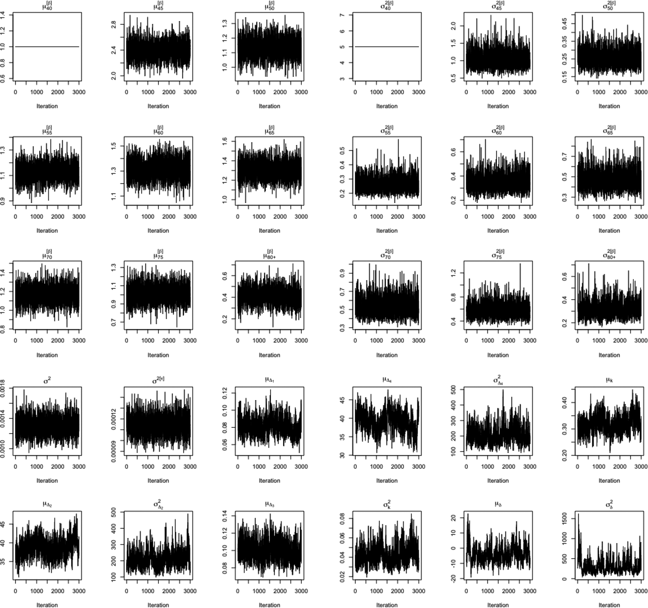
Traceplots for the hyperparameters in BHM for ASSAF.
Figure 13:
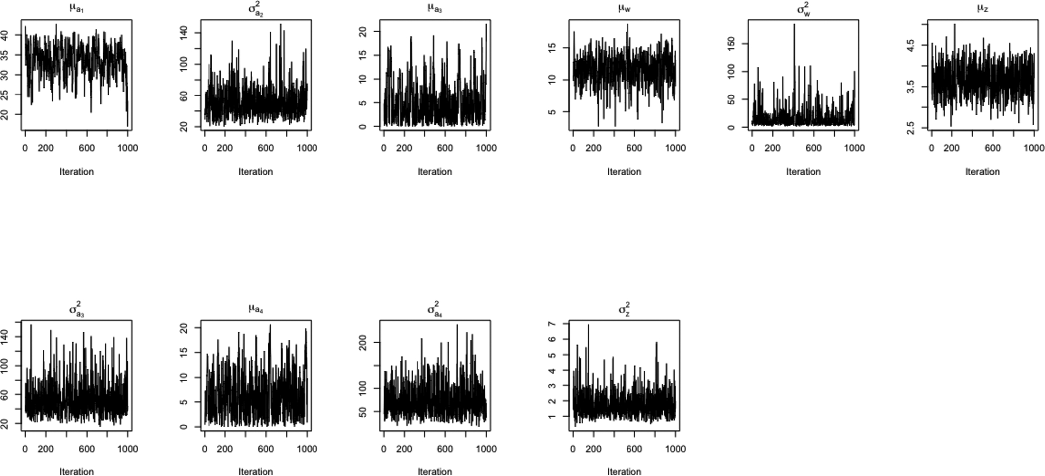
Traceplots for the hyperparameters in BHM for .
C. Forecast plots of all 69 countries
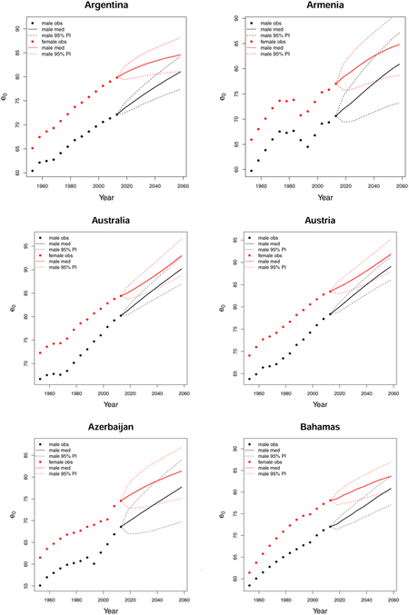
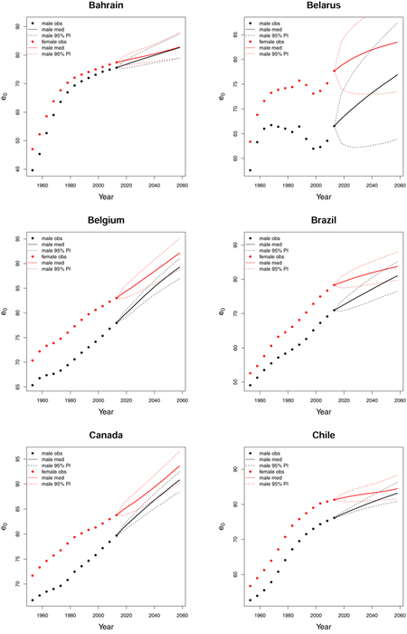
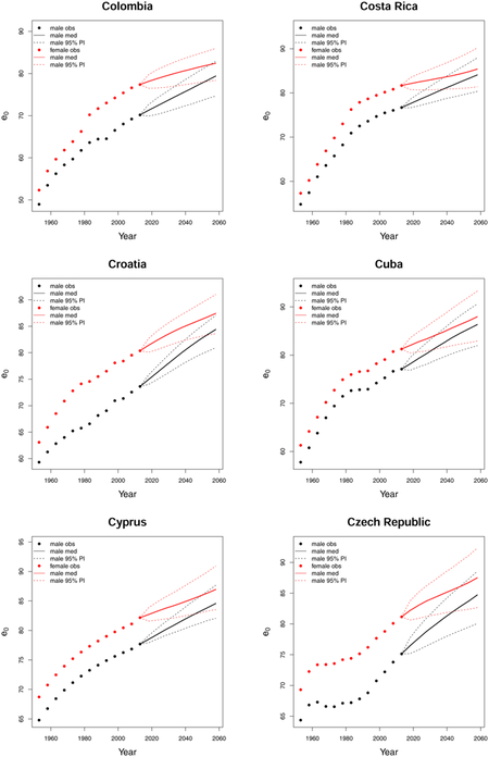
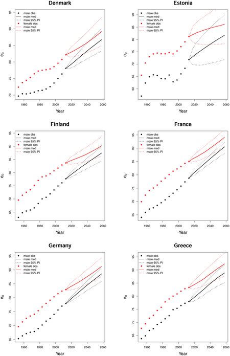
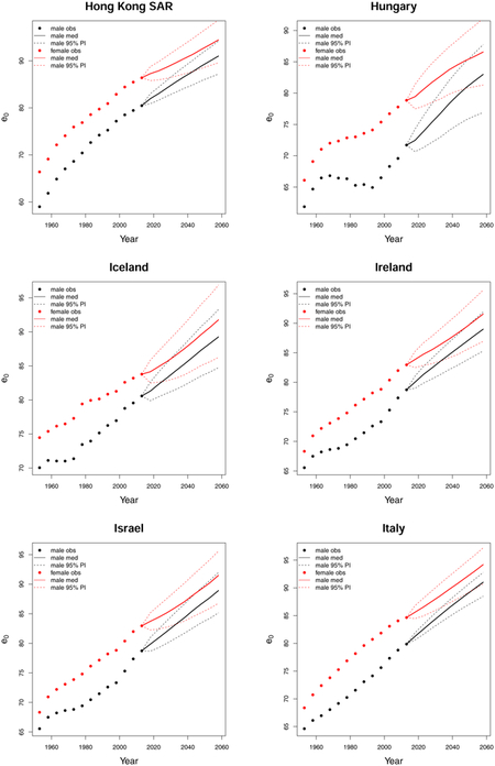
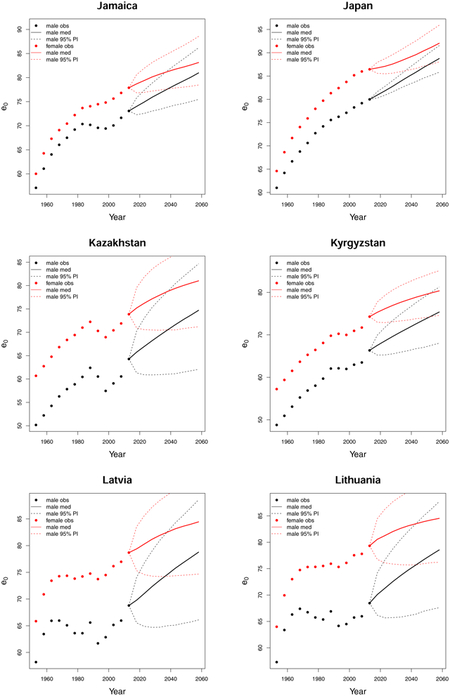
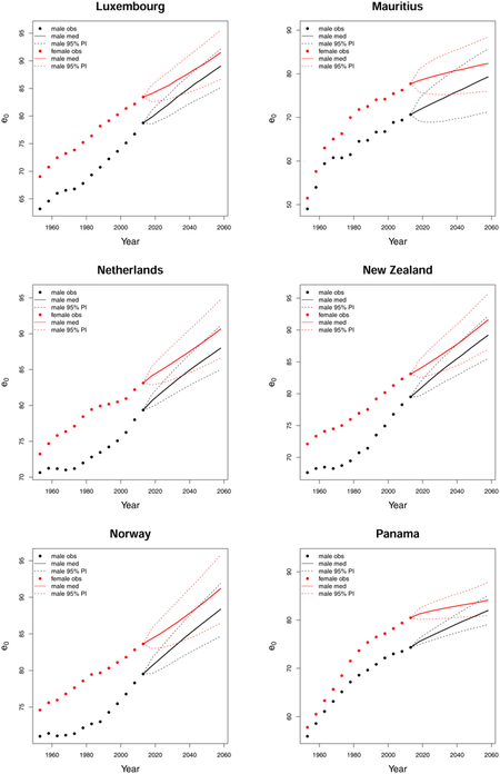
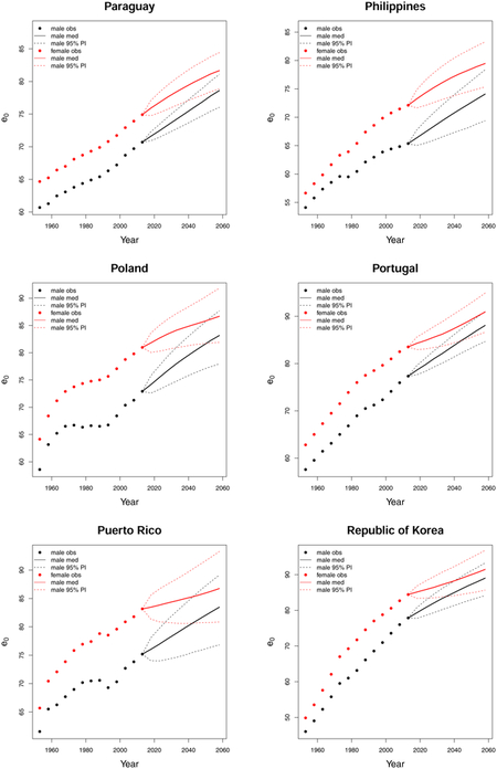
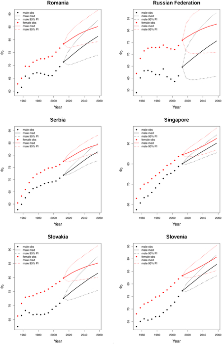
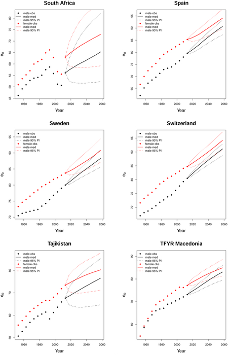
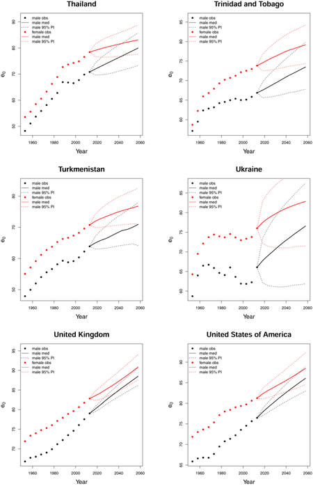
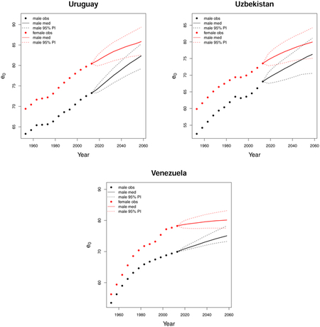
References
- Alkema L, Raftery AE, Gerland P, Clark SJ, Pelletier F, Buettner T, and Heilig GK (2011). Probabilistic projections of the total fertility rate for all countries. Demography, 48(3):815–839. [DOI] [PMC free article] [PubMed] [Google Scholar]
- Bongaarts J (2006). How long will we live? Population and Development Review, 32(4):605–628. [Google Scholar]
- Bongaarts J (2014). Trends in causes of death in low-mortality countries: implications for mortality projections. Population and Development Review, 40(2):189–212. [Google Scholar]
- Booth H, Hyndman RJ, Tickle L, and De Jong P (2006). Lee-Carter mortality forecasting: a multi-country comparison of variants and extensions. Demographic Research, 15:289–310. [Google Scholar]
- Britton J (2017). Death, disease, and tobacco. The Lancet, 389(10082):1861–1862. [DOI] [PubMed] [Google Scholar]
- Burns DM, Lee L, Shen LZ, Gilpin E, Tolley HD, Vaughn J, Shanks TG, et al. (1997). Cigarette smoking behavior in the United States. Changes in cigarette-related disease risks and their implication for prevention and control. Smoking and Tobacco Control Monograph, 8:13–42. [Google Scholar]
- Fokas N (2007). Growth functions, social diffusion, and social change. Review of Sociology, 13(1):5–30. [Google Scholar]
- Gneiting T and Raftery AE (2007). Strictly proper scoring rules, prediction, and estimation. Journal of the American Statistical Association, 102(477):359–378. [Google Scholar]
- Godwin J and Raftery AE (2017). Bayesian projection of life expectancy accounting for the HIV/AIDS epidemic. Demographic Research, 37:1549. [DOI] [PMC free article] [PubMed] [Google Scholar]
- Grübler A, Nakićenović N, and Victor DG (1999). Dynamics of energy technologies and global change. Energy Policy, 27(5):247–280. [Google Scholar]
- Hyndman RJ, Booth H, Tickle L, and Maindonald J (2019). Demography: Forecasting Mortality, Fertility, Migration and Population Data. R package version 1.22. https://CRAN.R-project.org/package=demography.
- Hyndman RJ and Ullah MS (2007). Robust forecasting of mortality and fertility rates: a functional data approach. Computational Statistics & Data Analysis, 51(10):4942–4956. [Google Scholar]
- Islami F, Torre LA, and Jemal A (2015). Global trends of lung cancer mortality and smoking prevalence. Translational Lung Cancer Research, 4(4):327. [DOI] [PMC free article] [PubMed] [Google Scholar]
- Janssen F (2018). Advances in mortality forecasting: Introduction. Genus, 74(1):21. [DOI] [PMC free article] [PubMed] [Google Scholar]
- Janssen F and van Poppel F (2015). The adoption of smoking and its effect on the mortality gender gap in Netherlands: a historical perspective. BioMed Research International, 2015. [DOI] [PMC free article] [PubMed] [Google Scholar]
- Janssen F, van Wissen LJ, and Kunst AE (2013). Including the smoking epidemic in internationally coherent mortality projections. Demography, 50(4):1341–1362. [DOI] [PubMed] [Google Scholar]
- King G and Soneji S (2011). The future of death in America. Demographic Research, 25:1–38. [DOI] [PMC free article] [PubMed] [Google Scholar]
- Kong KA, Jung-Choi K-H, Lim D, Lee HA, Lee WK, Baik SJ, Park SH, and Park H (2016). Comparison of prevalence-and smoking impact ratio-based methods of estimating smoking-attributable fractions of deaths. Journal of Epidemiology, 26(3):145–154. [DOI] [PMC free article] [PubMed] [Google Scholar]
- Kucharavy D and De Guio R (2011). Logistic substitution model and technological forecasting. Procedia Engineering, 9:402–416. [Google Scholar]
- Lee RD and Carter LR (1992). Modeling and forecasting US mortality. Journal of the American Statistical Association, 87(419):659–671. [Google Scholar]
- Lee RD and Miller T (2001). Evaluating the performance of the Lee-Carter method for forecasting mortality. Demography, 38(4):537–549. [DOI] [PubMed] [Google Scholar]
- Li N and Lee RD (2005). Coherent mortality forecasts for a group of populations: An extension of the Lee-Carter method. Demography, 42:575–594. [DOI] [PMC free article] [PubMed] [Google Scholar]
- Li Y and Raftery AE (2019). Estimating and forecasting the smoking-attributable mortality fraction for both sexes jointly in 69 countries. arXiv preprint arXiv:1902.07791 [DOI] [PMC free article] [PubMed] [Google Scholar]
- Marchetti C, Meyer PS, and Ausubel JH (1996). Human population dynamics revisited with the logistic model: how much can be modeled and predicted? Technological Forecasting and Social Change, 52(1):1–30. [DOI] [PubMed] [Google Scholar]
- Meyer P (1994). Bi-logistic growth. Technological Forecasting and Social Change, 47(1):89–102. [DOI] [PubMed] [Google Scholar]
- Oeppen J and Vaupel JW (2002). Broken limits to life expectancy. Science, 296(5570):1029–1031. [DOI] [PubMed] [Google Scholar]
- Pedroza C (2006). A Bayesian forecasting model: predicting US male mortality. Biostatistics, 7(4):530–550. [DOI] [PubMed] [Google Scholar]
- Peto R, Boreham J, Lopez AD, Thun M, and Heath C (1992). Mortality from tobacco in developed countries: indirect estimation from national vital statistics. The Lancet, 339(8804):1268–1278. [DOI] [PubMed] [Google Scholar]
- Preston S, Heuveline P, and Guillot M (2000). Demography: Measuring and Modeling Population Processes. Wiley-Blackwell. [Google Scholar]
- Preston SH and Wang H (2006). Sex mortality differences in the United States: The role of cohort smoking patterns. Demography, 43(4):631–646. [DOI] [PubMed] [Google Scholar]
- Raftery AE, Alkema L, and Gerland P (2014a). Bayesian population projections for the United Nations. Statistical Science, 29:58–68. [DOI] [PMC free article] [PubMed] [Google Scholar]
- Raftery AE, Chunn JL, Gerland P, and Ševčíková H (2013). Bayesian probabilistic projections of life expectancy for all countries. Demography, 50(3):777–801. [DOI] [PMC free article] [PubMed] [Google Scholar]
- Raftery AE, Lalic N, and Gerland P (2014b). Joint probabilistic projection of female and male life expectancy. Demographic Research, 30:795–822. [DOI] [PMC free article] [PubMed] [Google Scholar]
- Raftery AE and Lewis SM (1992). One long run with diagnostics: Implementation strategies for Markov chain Monte Carlo. Statistical Science, 7(4):493–497. [Google Scholar]
- Raftery AE, Li N, Ševčíková H, Gerland P, and Heilig GK (2012). Bayesian probabilistic population projections for all countries. Proceedings of the National Academy of Sciences, 109:13915–13921. [DOI] [PMC free article] [PubMed] [Google Scholar]
- Renshaw AE and Haberman S (2006). A cohort-based extension to the Lee-Carter model for mortality reduction factors. Insurance: Mathematics and Economics, 38(3):556–570. [Google Scholar]
- Rostron BL and Wilmoth JR (2011). Estimating the effect of smoking on slowdowns in mortality declines in developed countries. Demography, 48(2):461–479. [DOI] [PubMed] [Google Scholar]
- Ševčíková H, Li N, and Gerland P (2019a). MortCast: Estimation and Projection of Age-Specific Mortality Rates. R package version 2.1–1. https://CRAN.R-project.org/package=MortCast.
- Ševčíková H, Li N, Kantorová V, Gerland P, and Raftery AE (2016). Age-specific mortality and fertility rates for probabilistic population projections. In Dynamic Demographic Analysis, pages 285–310. Springer. [Google Scholar]
- Ševčíková H, Raftery A, and Chunn J (2019b). bayesLife: Bayesian Projection of Life Expectancy. R package version 4.0–2. https://CRAN.R-project.org/package=bayesLife.
- Shang HL (2016). Mortality and life expectancy forecasting for a group of populations in developed countries: a multilevel functional data method. The Annals of Applied Statistics, 10(3):1639–1672. [Google Scholar]
- Stoeldraijer L, Bonneux L, van Duin C, van Wissen L, and Janssen F (2015). The future of smoking-attributable mortality: the case of England & Wales, Denmark and the Netherlands. Addiction, 110(2):336–345. [DOI] [PubMed] [Google Scholar]
- Trias Llimós S and Janssen F (2019). Gender gaps in life expectancy and alcohol consumption in Eastern Europe. N-IUSSP. [DOI] [PubMed] [Google Scholar]
- United Nations (2015). World Population Prospects 2015. United Nations, New York, N.Y. [Google Scholar]
- United Nations (2017). World Population Prospects 2017. United Nations, New York, N.Y. Accessed: Oct. 15, 2018 http://population.un.org/wpp/Download/Standard/Population/. [Google Scholar]
- Vidr N., Trias-Llimó S., and Janss F. (2017). Impact of obesity on trends in life expectancy among different European countries, 1975–2012. European Journal of Public Health, 27(suppl 3). [Google Scholar]
- Wang H and Preston SH (2009). Forecasting United States mortality using cohort smoking histories. Proceedings of the National Academy of Sciences, 106(2):393–398. [DOI] [PMC free article] [PubMed] [Google Scholar]
- Whelpton PK (1936). An empirical method of calculating future population. Journal of the American Statistical Association, 31(195):457–473. [Google Scholar]
- Wiśniowski A, Smith PW, Bijak J, Raymer J, and Forster JJ (2015). Bayesian population forecasting: extending the Lee-Carter method. Demography, 52(3):1035–1059. [DOI] [PubMed] [Google Scholar]
- World Health Organization (2017). Mortality database. Last accessed: Oct. 15, 2018 http://www.who.int/healthinfo/statistics/mortality_rawdata/en/.


