Primary hybrid zone formation in Tephroseris helenitis (Asteraceae), following postglacial range expansion along the central Northern Alps

Abstract

Distinguishing between secondary versus primary hybrid zone formation remains a challenging task as, for instance, the time window in which these historical (vicariant) versus contemporary (environmental‐selective) processes are distinguishable may be relatively narrow. Here, we examine the origin and structure of a transition zone between two subspecies of Tephroseris helenitis along the central Northern Alps, using molecular (AFLP) and morphological (achene type) data in combination with ecological niche models (ENMs) to hindcast ranges at the Last Glacial Maximum (LGM) and mid‐Holocene. Samples were collected over a c. 350 km long transect, largely covered by ice during the LGM. Genetically nonadmixed individuals of subspp. helenitis versus salisburgensis dominated the westernmost versus eastern transect areas, with admixed individuals occurring in between. Clines for achene morphology and outlier loci potentially under climate‐driven selection were steep, largely noncoincidental, and displaced to the east of the cline centre for neutral AFLPs. During the LGM, ssp. helenitis should have been able to persist in a refugium southwest of the transect, while suitable habitat for ssp. salisburgensis was apparently absent at this time. Together with patterns of genetic and clinal variation, our ENM data are suggestive of a primary hybrid zone that originated after the species’ postglacial, eastward expansion. The observed clinal changes may thus reflect random/nonadaptive processes during expansion and selection on particular loci, and possibly achene type, in response to a long‐term, west‐to‐east climate gradient in the direction of more stressful (e.g., wetter/cooler) conditions. Overall, this study adds to the vast hybrid zone literature a rare example of a hybrid zone caused by primary differentiation within a plant species, underlaid by historical range expansion.

1. INTRODUCTION

Hybrid zones occur where individuals of populations or taxa differing in one or more diagnostic traits meet and cross‐fertilize (Arnold, 1997). Two main hypotheses are generally invoked to explain their origin and the phenotypic and/or genetic clines they create (reviewed in Abbott, 2017; Harrison & Larson, 2016): (a) secondary contact and admixture between partially reproductively isolated populations, following their divergence in allopatry (Barton & Hewitt, 1985), and (b) primary differentiation in parapatry due to spatially varying selection across an environmental gradient (Endler, 1977). The former explanation is traditionally favoured by the hybrid zone literature (Coyne & Orr, 2004). For instance, most studies in northern temperate regions indicate that hybrid zones, in both plants and animals, result from secondary contact of genetically distinct populations that expanded from previously isolated glacial refugia (e.g., Abbott, 2017; Barton & Hewitt, 1985; Hewitt, 2000; Scordato et al., 2017; see also Morales‐Rozo et al., 2017, for a tropical example). Often, but not always, such secondary contacts reflect “tension zones” as maintained by a balance between the homogenizing effect of dispersal into the zone and selection against hybrids (Abbott et al., 2018; Barton & Hewitt, 1985). In other instances, contact zones may have started their existence as “moving zones”, owing to strong asymmetric introgression from a local (“native”) taxon into an expanding one (reviewed in Wielstra, 2019). By comparison, primary hybrid zone formation across environmental gradients with continuous gene flow is rendered less likely (Abbott, 2017; Barton & Hewitt, 1985; Coyne & Orr, 2004). Nonetheless, some strong cases are documented for animals (reviewed in Johannesson, 2016; Ostevik et al., 2012) but less so for plants (e.g., Filatov et al., 2016; Schmickl & Koch, 2011).

Previous studies indicate that distinguishing between secondary contact versus primary differentiation remains a challenging task. For instance, early simulation (single‐locus or oligogenic) models presented by Endler (1977) showed that these essentially historical (vicariant) versus contemporary (environmental‐selective or “ecogenetic”) processes (sensu Thorpe, 1991) may produce similar clinal patterns unless observed “within the first few hundred generations” (cf. Harrison & Larson, 2016; see also Gompert & Buerkle, 2016). Nonetheless, stable tension zones induced by secondary contact should exhibit, at least initially, a set of spatially coincident/concordant clines (in terms of position/width) for all genetic or morphological traits that have diverged in allopatry (Barton & Hewitt, 1985; Durrett et al., 2000; Thorpe, 1991). Moreover, in a stable zone at migration‐selection equilibrium, the cline width for selectively neutral loci should not be greater than can be explained by dispersal rate and time since contact (Endler, 1977; see also McKenzie et al., 2015). By contrast, in a moving tension zone, asymmetric introgression for traits diagnostic of the native taxon should result in relatively steep and staggered clines, left behind as “trails” within the expanding taxon, i.e., predominantly in the area of initial contact viz. taxon displacement (Barton & Hewitt, 1985; Buggs, 2007; Currat et al., 2008; Wielstra, 2019; see also Wielstra et al., 2017). However, spatially congruent or staggered clines are not necessarily expected in a primary hybrid zone, unless many independent traits/loci respond in a similar fashion to sharp changes in one or more environmental factors (Durrett et al., 2000). Accordingly, if a single species has expanded its range (e.g., from a single glacial refuge) over an environmental gradient, we might expect that divergent selection on different traits and loci would mostly result in clines with different positions and/or widths (Futuyma, 2005; Johannesson, 2016). In this instance, the evidence becomes stronger if (a) selectively neutral variation displays a clinal pattern in the direction of postglacial spread (Hewitt, 1999), and (b) an allopatric phase can be rejected (Abbott, 2017). Such a scenario of primary hybrid zone formation, following postglacial range expansion, has not been extensively researched empirically (though see Antoniazza et al., 2010; Filatov et al., 2016; Vasemägi, 2006).

In this study, we use population genetic and phenotypic approaches combined with geographical cline analyses and palaeodistribution modelling to illuminate the origin and structure of a putative hybrid zone formed by the short‐lived perennial Tephroseris helenitis (L.) B. Nord. (Asteraceae, Senecioneae) in the forelands of the central Northern Alps. Here, ssp. helenitis, which represents much of the species’ West/Central European range, is gradually replaced by ssp. salisburgensis (Cuf.) B. Nord., a local endemic of Southeast Germany and North‐Central Austria (e.g., Meusel & Jäger, 1992; GBIF.org; see Figure 1a,b). Throughout this transition zone, which runs more or less linearly over c. 150 km along the Bavarian–Salzburg Alps, both subspecies inhabit seasonally wet meadows and fens on calcareous to peaty soils at moderate elevations, c. 400–800 m (Fischer et al., 2008; Stöhr, 2009; Table S1). While genetic and experimental (e.g., crossing) evidence is lacking, the two taxa are distinguishable in various quantitative traits (e.g., leaf shape, stem/bract coloration, ray floret number) (Chater & Walters, 1976). Their main diagnostic feature, however, is fruit (achene) indumentum, which is pubescent in ssp. helenitis and glabrous or sparsely hairy in ssp. salisburgensis (Cufodontis, 1933; Figure 2).

FIGURE 1.

(a) Simplified map showing the distribution of Tephroseris helenitis ssp. helenitis in West/Central Europe (blue area), and the peripheral eastern range of ssp. salisburgensis (pink area), based on georeferenced locality records per taxon (n = 1005 vs. 138) from the Global Biodiversity Information Facility (GBIF.org). (b) Detailed map of the helenitis–salisburgensis hybrid zone in the central North‐Alpine forelands (South Germany, Salzburg Federal State, western Upper Austria). Coloured symbols indicate GBIF records for ssp. helenitis (n = 426; blue squares), ssp. salisburgensis (n = 137; pink triangles), and T. helenitis without infraspecific rank (n = 1556; small black dots; GBIF.org; 10 December, 2019; https://doi.org/10.15468/dl.ogvvpp). White circles represent 29 of the 30 populations surveyed for achene type and/or genetic variation in three defined collection sectors (west, central, east) and projected onto a defined transect (black solid line) used for cline fitting analysis. Note, population no. 3 lies off this map, c. 204 km north of population no. 2. Numbers at the bottom correspond to population numbers as identified in Table S1. The black dashed line shows the extent of the northern Alpine glaciers (plus localized ice caps in the Bohemian Forest) at the Last Glacial Maximum (LGM, c. 24.5–18 ka BP) according to Ehlers et al. (2011) [Colour figure can be viewed at wileyonlinelibrary.com]

FIGURE 2.

Fruit (achene) indumentum variation among the two Tephroseris helenitis subspecies of this study. (a) Pubescent achene with hairs (trichomes) on the entire surface, as diagnostic for ssp. helenitis. (b) Entirely glabrous achene, or (c) sparsely hairy achene with few trichomes on individual grooves, as both diagnostic for ssp. salisburgensis. Photographs were obtained with a Leica DVM6 z‐stacking digital microscope (Leica Microsystems) [Colour figure can be viewed at wileyonlinelibrary.com]

There are two main reasons why this subspecies transition offers an interesting setting for unravelling historical‐demographic and environmental‐selective processes potentially at work in hybrid zones. First, it presently coincides with a marked west‐east climate gradient along the Bavarian‐Salzburg Alps, especially in mean annual precipitation, c. 900 mm (west) to 1300 mm (east) (Table S1; see also Isotta et al., 2013). Particular gene loci might therefore be subject to differential, climate‐induced selection, as could also apply to variation in achene indumentum, given its potential role, for instance, in germination (e.g., Kreitschitz, 2012) and presumably strong genetic basis (e.g., Cui et al., 2016; Rollins, 1958). Second, during the Last Glacial Maximum (LGM, c. 24,500–18,000 years before present, BP), much of this transition zone was covered by the terminal lobes of various Alpine glaciers (Ehlers et al., 2011; see Figure 1b). Hence, the question arises of whether ancestral forms colonized deglaciated terrain from disjunct refugia or out of a single, continuous refugium, as predicted by the secondary contact and primary differentiation hypotheses, respectively (Antoniazza et al., 2010; Morales‐Rozo et al., 2017).

Accordingly, the two overarching aims of this study were to evaluate these two hypotheses and to gain further insights into the historical/neutral and adaptive/ecogenetic processes underlying this subspecies transition. To accomplish this, we (a) surveyed 29 populations of T. helenitis over a c. 350 km‐long transect along the central Northern Alps for amplified fragment length polymorphisms (AFLPs; plus a single, more northerly population; Figure 1b), (b) recorded achene type variation at 28 of those sites, (c) tested for non‐neutral (outlier) locus‐by‐climate and ‐phenotype associations as potential signatures of local adaptation, and (d) employed geographical cline fitting analyses for estimating the position and width of individual character clines (neutral AFLPs, achene type, outlier loci). Finally, we sought to infer the historical dynamics of this putative hybrid zone by reconciling patterns of population genetic variation with taxon‐specific palaeodistribution models for both the LGM and the mid‐Holocene Climate Optimum (c. 6 ka BP).

2. MATERIALS AND METHODS

2.1. Study sites, sampling design and achene type survey

Based on the floristic literature (e.g., Stöhr, 2009) and our own field surveys, 30 populations of Tephroseris helenitis were chosen as sampling sites in the central North‐Alpine forelands of South Germany, Salzburg Federal State and western Upper Austria (Figure 1b, Table S1; see also Method S1 for detailed descriptions of the distribution, taxonomy and biology of T. helenitis). For ease of reference, populations were assigned to three collection sectors (west, central, east). These included seven populations (nos. 1–7) from the western core region of ssp. helenitis, including one (no. 3) from a more northern locality in South Germany/Bavaria (c. 204 km north of no. 2; mapped in Figure S1 and serving as reference parental sample); five (nos. 8–12) from the “central” region of putative range overlap with ssp. salisburgensis; and 18 populations (nos. 13–30) from the supposed ”eastern” core region of the latter taxon. To reduce spatial dimensionality for cline fitting analyses (see below), we defined a c. 350 km‐long transect between western‐ and easternmost populations (Figure 1b) and projected the remainder onto this line, using the “distance to nearest hub” algorithm in qgis 3.8 (QGIS Development Team, 2019; see also McEntee et al., 2016).

Achene type was examined in 28 populations (excepting nos. 13 and 21) with on average 20.8 (±9.7 SD) individuals per site (in total n = 582) by recording the surface indumentum (pubescent vs. glabrous/sparsely hairy) of at least five achenes per individual using a magnifying glass or stereomicroscope (Table 1). Accordingly, all seven western populations and one from the central region (no. 9) were a priori classified as “nominally” ssp. helenitis; four central and 11 eastern populations as “mixed” (i.e., when the rare achene type occurred with frequency ≥5%); and five eastern populations as “nominally” ssp. salisburgensis (Table 1). All achenes within a given individual displayed the same type (G. Pflugbeil, personal observation).

TABLE 1.

Summary of achene type and genetic (AFLP) characteristics for 28 and 30 populations of Tephroseris helenitis, respectively, sampled across the helenitis–salisburgensis hybrid zone along the central Northern Alps (South Germany, Salzburg Federal State, western Upper Austria), including one northerly population (no. 3; see also Figure 1b and Table S1 for detailed locality information)

Sector/population no. a	N (morph)	Achene morphs (relative frequency)		Locality type	n (AFLP)	PPF	HE	DW b
		Pubescent	Glabrous/sparsely hairy					30 sites	24 sites
West
1	21	1.00	0.00/0.00	Hel	10	44.30	0.164	2.643H	2.893H
2	10	1.00	0.00/0.00	Hel	9	37.06	0.141	2.349H	2.540H
3	5	1.00	0.00/0.00	Hel	5	35.96	0.174	1.895	2.072
4	20	1.00	0.00/0.00	Hel	8	41.45	0.167	1.895	2.075
5	20	1.00	0.00/0.00	Hel	8	48.68	0.199	2.879H	3.343H
6	17	1.00	0.00/0.00	Hel	4	39.04	0.214	2.568H	NA
7	18	1.00	0.00/0.00	Hel	4	37.72	0.206	2.589H	NA
Central
8	21	0.86	0.05/0.09	Mixed	5	33.55	0.161	1.539L	1.706L
9	15	1.00	0.00/0.00	Hel	11	48.46	0.173	1.645L	1.833L
10	20	0.80	0.15/0.05	Mixed	6	31.36	0.141	1.657	1.844
11	22	0.82	0.00/0.18	Mixed	5	37.94	0.187	2.088	2.335
12	23	0.30	0.61/0.09	Mixed	5	41.45	0.204	2.159	2.398
East
13	NA	NA	NA	NA	8	48.03	0.187	2.007	2.230
14	20	0.35	0.50/0.15	Mixed	18	64.91	0.194	2.054	2.305H
15	14	0.21	0.72/0.07	Mixed	8	49.78	0.199	2.067	2.283
16	5	0.00	0.60/0.40	Sal	4	32.02	0.174	2.071	NA
17	31	0.26	0.55/0.19	Mixed	7	45.83	0.193	2.356H	2.704H
18	20	0.15	0.75/0.10	Mixed	8	45.83	0.184	1.658L	1.865
19	34	0.56	0.35/0.09	Mixed	9	52.41	0.198	2.226H	2.433H
20	50	0.26	0.60/0.14	Mixed	15	53.51	0.172	1.414L	1.561L
21	NA	NA	NA	NA	2	18.20	0.182	1.849	NA
22	20	0.00	1.00/0.00	Sal	17	55.70	0.174	1.686L	1.839L
23	30	0.07	0.76/0.17	Mixed	9	44.74	0.173	1.844	1.995
24	32	0.03	0.91/0.06	Sal	7	34.43	0.143	1.271L	1.385L
25	13	0.23	0.62/0.15	Mixed	4	32.02	0.180	1.911	NA
26	10	0.00	1.00/0.00	Sal	5	31.14	0.155	1.556L	1.713L
27	32	0.00	0.94/0.06	Sal	3	24.78	0.165	1.964	NA
28	29	0.21	0.66/0.14	Mixed	10	42.98	0.160	1.469L	1.614L
29	10	0.20	0.80/0.00	Mixed	7	41.01	0.170	2.241H	2.449H
30	20	0.10	0.90/0.00	Mixed	12	44.08	0.156	1.482L	1.631L
Species total	582				233	98.46	0.206
Species mean	20.8 (9.7)				7.8 (3.8)	41.28 (9.64)	0.176 (0.019)

N refers to the number of individuals surveyed for achene type (morph) and genetic (AFLP) variation. Shown are the relative frequencies of achene morphs (ssp. helenitis: pubescent; ssp. salisburgensis: glabrous/sparsely hairy). Based on this, the locality type specifies whether a given locality contained individuals of ssp. helenitis (hel), ssp. salisburgensis (sal) or both taxa (mixed, i.e., when the rare achene type occurred with frequency ≥5%).

Abbreviations: DW, frequency down‐weighted marker values, calculated separately for all 30 populations (n = 233) as well as 24 populations (n = 212) with n ≥ 5; H _E, Nei’s (1987) unbiased gene diversity; n, number of individuals; NA, not analysed; PPF, percentage of polymorphic fragments.

^aMembership of the populations to a priori defined collection sectors (see also Figure 1b, and text for details).

^bSignificantly low or high DW values are indicated by superscripts “L” and “H”, respectively. Note: Populations are sorted by longitude, starting with the westernmost population no.1. Standard deviations are shown in parentheses.

For genetic analyses, 338 individuals representing all 30 populations (and including plants scored for achene type) were sampled for silica‐dried leaf material. Voucher specimens of all populations studied are stored at the Herbarium of Salzburg University (SZU).

2.2. Characterization of local climate in relation to achene type variation

Climate variation across the 30 sampling sites was investigated by principal components analysis (PCA) in past 3.25 (Hammer et al., 2001), using 19 bioclimatic variables (bio1–19) from worldclim 1.4 (http://www.worldclim.org/) with 30 arc‐seconds resolution for current conditions (c. 1950–2000) at each site. For the 28 sites of known achene type, we used univariate linear regressions in r 3.6.1 (R Development Core Team, 2017) to test for a significant relationship between the proportion of pubescent (helenitis) achene‐plants (dependent variable) and ordinated climate space, as described by standardized PCA scores per site based on the first two components (PC1, PC2), respectively (explanatory variables).

2.3. DNA extraction and AFLP genotyping

Total genomic DNA was extracted from leaf tissue using DNeasy Plant Mini Kit (Qiagen). The AFLP analysis followed Vos et al. (1995), with minor modifications for the use of fluorescent‐dye‐labelled primers (Jaros et al., 2016). Based on an initial selective primer trial on eight individuals using 18 primer pair combinations (data not shown), the following three were chosen for the full survey: EcoRI‐AGC/MseI‐CAG (NED), EcoRI‐ACG/MseI‐CAT (VIC), and EcoRI‐AGA/MseI‐CAC (6‐FAM). Each PCR plate (48 slots) contained one positive control (“between‐run‐replicate”), one negative control (“within‐plate‐replicate”), and one blind sample. The selective PCR products were purified using Sephadex g‐50 Superfine (GE Healthcare BioSciences). Fragments were separated on a MegaBACE 1000 (GE Healthcare BioSciences), using the ET550‐R‐Rox‐MegaBACE sizing standard, and manually scored as presence (1) or absence (0), using dax 8.0 (Van Mierlo Software Consultancy; see also Bendiksby et al., 2011). The sums of mismatches among five positive and five negative controls were used to obtain an AFLP error rate according to Bonin et al. (2007). Individuals were excluded sequentially from the data set (in total n = 338) if they (a) failed to amplify in at least one of the three primer combinations (n = 54); (b) showed c. 50% longer branches than typical samples in a preliminary genetic distance tree (n = 7); and (c) had more or fewer fragments than the overall mean (± SD) per individual (148.5 ± 27.7; n = 44; data not shown). The final AFLP data set comprised 233 individuals (n = 7.8 ± 3.8 per site; Table 1), including 216 samples of known achene type (92.7% of the total).

2.4. Analysis of population genetic diversity and differentiation

Based on all 456 AFLP loci (including monomorphic ones), measures of within‐population diversity were calculated by the percentage of polymorphic fragments (PPF) and Nei’s (1987) unbiased gene diversity (H _E), using genalex 6.5 (Peakall & Smouse, 2012). In addition, we estimated “frequency‐down‐weighted marker‐values” (DW; or “rarity”) for each population, using the aflpdat r package (Ehrich, 2006), with significance estimated over 1000 permutations. Spearman's rank correlations were employed to test for a potential relationship between each genetic parameter (PPF, H _E, DW) and longitude per site (see Table S1). For DW, we also tested whether insufficient within‐population sampling affected estimates and correlation analyses by comparing results for all 30 populations and only those (24) with sample sizes n ≥ 5 (Table 1). As an overall measure of population subdivision, we calculated Φ _PT (an analogue of F _ST) from analysis of molecular variance (AMOVA) in genalex, with significance estimated over 9999 permutations. Using the same program, we tested for isolation‐by‐distance (IBD) through a Mantel test (9999 permutations) between pairwise Φ _PT/(1‐Φ _PT) values of populations and their log₁₀‐transformed geographical distances (in km; Rousset, 1997).

2.5. Spatially explicit analysis of genetic admixture

For the estimation of hybrid index values (see below), we first approximated which of the 30 populations best represent the “pure” (nonadmixed) genetic backgrounds of each subspecies. To this aim, we performed individual‐based Bayesian clustering on the polymorphic (hereafter “total”) AFLP data set (n = 233, 449 loci), using tess 2.3.1 (Durand et al., 2009). In contrast to similar approaches (e.g., structure), the tess algorithm uses a spatially explicit model that incorporates geographical coordinates of individuals as prior information, as particularly suitable for differentiating between clinal (e.g., intraspecific) transitions and more abrupt breaks between hybridizing (e.g., interspecific) genetic groups that evolved in allopatry (Buchalski et al., 2016). We ran tess under the conditional autoregressive (CAR) Gaussian model of admixture with a linear trend surface for dominant markers (recessive allele model), using default parameters (admixture parameter, α = 1.0; spatial interaction parameter, ψ = 0.6), and with exact (nonprojected) locality coordinates included as prior (see Table S1). For each number of clusters (K) tested (2–10), we conducted 10 Markov chain Monte Carlo (MCMC) runs of 5 × 10⁶ iterations after a burn‐in of 50,000 steps. Individual cluster membership probabilities (q‐values) from the 10 replicates for each K were averaged using clumpp 1.1.2 (Jakobsson & Rosenberg, 2007). According to the tess manual, the optimal K might be determined as the point at which the mean values of the Deviance Information Criterion (DIC) over replicate runs level off or stabilize. Because this approach tends to overestimate the effective number of clusters (Durand et al., 2009), we also considered a value of K as optimal if an increase in K did not result in a clear additional cluster (Basto et al., 2016). Based on the favoured model (K = 2; see Results), values of q were examined for nonadmixed individuals (q ≥ 0.90 for either parental cluster) and admixed (“hybrid”) individuals (0.10 ≤ q < 0.90; McKenzie et al., 2015). In addition, we used the geospatial interpolation technique implemented in tess (“universal kriging”; Durand et al., 2009; Ripley, 1981) to predict admixture values for nonsampled geographical sites, based on simple kriging of the posterior probability of cluster memberships at each sampled location.

2.6. Potential loci under selection and tests of locus‐by‐climate/achene type associations

For the detection of potential loci under selection (so‐called F _ST outlier loci), we implemented both the fdist 3.5 (Excoffier & Lischer, 2010) and bayescan 2.1 (Foll & Gaggiotti, 2008) approaches for dominant binary data on the total AFLP data set (449 loci; see Method S2 for details). To account for false‐positive identification of outliers (e.g., Foll & Gaggiotti, 2008), we retained only those supported by both programs. To further elucidate the potentially adaptive nature of the three jointly identified loci (see Section 3), we linearly regressed their fragment (“allele”) frequencies per site (as calculated in genalex) on individual predictor variables of climate (bio1–19, PC1 and PC2 scores; 30 sites) and phenotype (helenitis‐achene type frequency; 28 sites).

2.7. Calculation of hybrid index values

For the calculation of hybrid index (HI) values, two westernmost populations of “nominally” ssp. helenitis (nos. 1, 2) and two easterly populations of ssp. salisburgensis (nos. 22, 24) were chosen to represent each taxon, based on three criteria: (a) sufficiently large sample size (n ≥ 7), (b) essentially nonadmixed ancestry, with mean q‐values ≥0.90 (range 0.90–1.0) for either parental cluster, based on the tess results, and (c) fixation or at least predominance (frequency >90%) of diagnostic achene types (Table 1). These four populations served as “parental” types to train the program introgress 1.1 (Gompert & Buerkle, 2010), using the “prepare.data” function for dominant markers. Maximum likelihood estimates of individual HI values were then calculated (function “est.h”) and averaged for each population using the fragment (“allele”) frequency differentials (δ) of the samples representing each “parent”. All estimates were scaled between 1 (“helenitis”) and 0 (“salisburgensis”), with intermediate values indicating genetically admixed individuals. For comparison, we also calculated HI values from the neutral AFLP data set with outlier loci excluded.

2.8. Geographical cline analyses

We used the Metropolis‐Hastings MCMC algorithm implemented in the r package hzar (Derryberry et al., 2014) to fit a series of geographical cline models to six data sets, including: (a) the mean HI values for all 30 populations, based on the total versus neutral AFLPs (449 vs. 446 loci), (b) the relative frequencies of the helenitis‐achene type (pubescent) in 28 populations, and (c) the fragment (“allele”) frequencies at each of the three outlier loci (for 30 populations). For each data set, we ran three separate models, all of which estimated cline centre (c; in km along the fitted transect, starting from population no. 1) and width (1/maximum slope, w) as well as 2log‐likelihood unit support limits (confidence intervals; CIs) around these estimates. We tested three commonly used models (I–III; Brumfield et al., 2001; McKenzie et al., 2015), which include combinations of fixing or estimating minimum and maximum data values at the cline ends (p _min, p _max) (models I vs. II, III), either with or without fitting of exponential tails (models I, II vs. III). We ran each model for three independent MCMC chains (100,000 iterations per chain) and compared them to each other and a null model of no clinal transition, using the corrected Akaike Information Criterion (AIC_c). The best‐fit model was determined through the lowest AIC_c score (McKenzie et al., 2015). We considered cline centres with nonoverlapping CIs to be significantly different (i.e., noncoincident); similarly, we regarded the widths of two clines to be significantly different (i.e., nonconcordant) if the upper CI of the narrower cline did not overlap with the lower CI of the broader one (Scordato et al., 2017). As total and neutral AFLP data sets generated almost identical cline shape parameters (data not fully shown), only the latter will be considered here.

Finally, we compared our estimated cline width for neutral AFLPs with the width of a neutral cline expected for a stable tension zone at dispersal‐selection equilibrium. In this scenario, neutral, unlinked loci should produce relatively narrow clines, unless dispersal rates are very high and/or a long time has elapsed since secondary contact (Barton & Hewitt, 1985; Endler, 1977). Hence, the width of such a neutral cline (ɷ*) might be predicted from Endler’s (1977) equation: ɷ* = 2.51 σ (sqrt T), where σ is the dispersal distance per generation and T the number of generations since contact (see also Barton & Gale, 1993). To do this, we assumed (a) a generation time of two years for T. helenitis, as observed in open cultivation (G. Pflugbeil, personal observation), (b) σ values of 0.24 or 0.54 km, as estimated for other short‐lived and wind‐dispersed perennials of Senecioneae using linkage disequilibrium (Brennan et al., 2009), and (d) c. 3000 or 9000 generations since hypothetical contact (c. 6 or 18 ka BP; see ENM results).

2.9. Present and past distribution modelling

We generated present and past ecological niche models (ENMs) in maxent 3.4.1 (Phillips et al., 2017) for each subspecies to determine whether their ranges were either disjunct or continuous in the past, as predicted by the secondary contact versus primary differentiation hypotheses. Information on the geographic distribution of each taxon was based on (a) the eight versus five “nominal” populations of subspp. helenitis versus salisburgensis, as defined by achene type (see Table 1), and (b) georeferenced locality records per taxon from the Global Biodiversity Information Facility (GBIF.org; 30/31 October 2019; https://doi.org/10.15468/dl.4igkbk and https://doi.org/10.15468/dl.i32en4, respectively). Records outside known taxon ranges were filtered out. In addition, we removed localities within a 2.5 km radius to account for spatial sampling bias, resulting in 432 locality records of ssp. helenitis and 66 of ssp. salisburgensis.

The current distribution of each taxon was modelled in maxent using 12 bioclimatic layers at 2.5 arc‐minutes resolution (bio2, 3, 7–11, 15–19; Table S2), i.e., after removing highly correlated variables (Pearson's r > |.85|) in enmtools 1.4.4 (Warren et al., 2010) to avoid potential over‐fitting. Each model was projected onto palaeoclimatic data sets simulated by the Model for Interdisciplinary Research on Climate (MIROC) for, respectively, the mid‐Holocene Climate Optimum (HCO, c. 6 ka BP; MIROC‐ESM; http://www.worldclim.org/) and the LGM (c. 22 ka BP; MIROC‐ESM; http://www.worldclim.org/). Present‐day distributions were modelled 10 times, using different subsets of 75% of the localities to train the model. For each run, model accuracy was evaluated for both training and testing data using the area under the curve (AUC) of the receiver operating characteristic (ROC) plot (good: 0.75 < AUC ≤ 0.92; very good: 0.92 < AUC ≤ 0.97; excellent: 0.97 < AUC ≤ 1.00; Hosmer & Lemeshow, 2000), with high similarity between training and testing values indicating low risk of model overfitting (Fois et al., 2018).

3. RESULTS

3.1. Among‐site variation in climate and achene type

In the PCA of the 30 sampling sites based on 19 bioclimatic variables (Figure 3), the primary loadings (>~|0.8|) of the first axis (PC1; 52.7% of the total variance) largely captured a west‐to‐east continuum of increasingly higher precipitation (bio12–14, 16–19) with stronger (e.g., seasonal) temperature fluctuations (bio2–4, 7) and lower minimum winter temperature (bio6); by contrast, PC2 (28.2%) primarily described other aspects of temperature (bio1, 5, 8, 10, 11), with lowest values in the central and far eastern portions of the transect (see Table S2 for loadings). The proportion of pubescent (helenitis) achene morphs, as estimated for 28 sites, decreased from west to east (see pie‐charts in Figure 3), as likewise predicted by among‐site variation in climate scores for PC1 (regression coefficient β = −0.36, p < .001) but not PC2 (β = −0.07, p = .359).

FIGURE 3.

Principal components analysis (PCA) biplot for 30 sampled sites of Tephroseris helenitis based on 19 bioclimatic variables (bio1–19; http://www.worldclim.org/). Twenty‐eight of those sites (except nos. 13 and 21; black dots) are represented by pie‐charts showing the relative frequencies of “helenitis” (light blue) versus “salisburgensis” (red) achene morphs (see Table 1). Percentages of total variance explained by each component are shown in parentheses. Convex hulls depict the smallest area occupied by populations assigned to three defined collection sectors (west, central, east; see Figure 1b and text). Population numbers are identified in Table S1. See Table S2 for loadings and identification of bioclimatic codes [Colour figure can be viewed at wileyonlinelibrary.com]

3.2. Population genetic diversity and differentiation

Our AFLP survey of the 30 Tephroseris helenitis populations (n = 233) yielded a total of 456 unambiguous fragments (range: 77–582 bp), of which 449 markers (loci) were polymorphic (PPF = 98.46%; Table 1). The three different primer pairs generated a variable number of fragments (“NED”: 98; “VIC”: 150; “6‐FAM”: 208), with an average (±SD) of 152 ± 55 fragments per primer combination. The overall error rate calculated from 10 replicates (3.6%) was within the typical range (2%–5%) reported for other AFLP studies in plant species (Poelchau & Hamrick, 2012).

Levels of within‐population genetic diversity (PPF, H _E) varied but were quite similar across populations (Table 1). Considering only populations with n ≥ 5, estimates of PPF and H _E ranged from 31.4 to 64.9 (mean: 49.3) and 0.141 to 0.204 (mean: 0.173), respectively. Significantly high estimates of rarity (DW) were found in populations from both the western and eastern collection sectors, yet only central and eastern sites had significantly small DW values, regardless of whether 30 or 24 populations were considered (Table 1). As a result, rarity was negatively corelated with longitude (30/24 populations: r = −.478/−.478, p = .008/.022) but not with PPF or H _E (all p values = .221–.600). Genetic differentiation across all 30 populations was moderate but significant (Φ _PT = 0.154, p < .001) and strongly associated with a pattern of IBD (r _M = 0.629, p < .001).

3.3. Spatial patterns of genetic admixture in relation to achene type variation

In the tess admixture analysis of the total AFLP data set (n = 233, 449 polymorphic loci), the plot of DIC values for K = 2–10 started to level off and stabilize at K ≥ 3 (Figure S2a). However, bar‐plots for K = 2–5 revealed no clear additional genetic structure for K > 2 (Figure S2b). We thus considered K = 2 as the best solution. The corresponding bar‐plot (Figure 4a) clearly showed a clinal transition of individual assignment (q) probabilities across the sampled sites for putative parental clusters I (“helenitis”) versus II (“salisburgensis”), as likewise confirmed by interpolation maps, predicting admixture values of each cluster for nonsampled sites (Figure S1). However, on closer inspection (Figure 4a), only the two westernmost populations of “nominal” ssp. helenitis (nos. 1, 2) were nearly fixed for cluster I (mean q = 0.91, n = 19). The remaining western populations (nos. 3–7) and all central ones (nos. 8–12) showed high admixture proportions (mean q = 0.37, n = 61), and most individuals from the eastern “core” populations of ssp. salisburgensis (nos. 13–30) were assignable to cluster II (mean q = 0.96, n = 153). By contrast, as shown in Figure 4b, the vast majority of genotyped individuals with known achene type from the west/central regions had the “helenitis” type (73/76, 96.1%), while this was the case for only a minority of those from the east (27/140, 19.3%). These patterns of achene type variation were also in broad agreement with the spatial variation of this phenotypic marker in the field (Figure 3).

FIGURE 4.

Genetic structure of the helenitis–salisburgensis hybrid zone based on the spatially explicit tess admixture analysis of the total AFLP data set (449 loci) of 30 populations (n = 233). (a) Bar plot for the favoured model, K = 2, indicating the clusters of “helenitis” (I, orange) versus “salisburgensis” (II, purple). The y‐axis presents membership probabilities (q‐values) for each individual, as represented by the smallest vertical bar. The x‐axis corresponds to population numbers. See Figure S2 for the corresponding DIC curve and bar‐plots for K = 3–5. (b) Assignment of “helenitis” versus “salisburgensis” achene types to 216 (out of 233) genotyped individuals from (a), with white bars indicating those of unknown phenotype [Colour figure can be viewed at wileyonlinelibrary.com]

3.4. Potential loci under selection and their climate/achene type associations

Using fdist, we identified 15 loci (3.3% of the total), with F _ST values above/below the 1% quantile, including nine loci under diversifying selection and six under balancing selection, while the bayescan approach inferred nine divergently selected loci (2%) with log₁₀(q) values ≤−2 (see Figure S3a,b; Table S3). However, only three loci (L152, L229, L257), each under diversifying selection, were detected by both methods. Nonetheless, their potentially adaptive nature was indicated by the large number of significant regression coefficients for 10 and up to 13 (out of 19) bioclimatic variables (after sequential Bonferroni correction at α = 0.05). The latter included descriptors of temperature (bio2–7) and precipitation (bio12–14, bio16–19), as well as for overall climate (PC1) space and achene type (all p < .001; see Table S4).

3.5. Geographical cline fitting analyses

According to hzar, the data sets of neutral AFLPs (446 loci) and achene type best‐fitted model I, while model II provided the best fit for each outlier locus (Table 2). As shown in Figure 5a, the AFLPs generated a smooth, broad cline (c. 352 km), centred in the middle of the transect (at c. 173 km; near site 7). By contrast, the achene cline was much steeper, sigmoid, and relatively narrow (c. 113 km); its centre was estimated at c. 270 km (site 12), indicating an eastward shift relative to the neutral cline. The same was true for all three outlier loci (Figure 5b), but which produced sharply narrow, step‐like clines, ranging from c. 1–2 km (L152, L229) to 38 km (L257). Those of L152 and L257 had their centres at c. 213–219 km (sites 9–11), while the cline centre for L229 was located at c. 300 km (sites 13–18; Table 2). Considering CIs around estimates (see superscript letters in Table 2 for pairwise comparisons), these analyses revealed: (a) significant differences in centre (noncoincidence) among the clines for AFLPs, achene type, L152/L257 and L229, and (b) significant differences in cline width (nonconcordance) for AFLPs, achene type/L257 and L152/L229, but not among the three outlier loci themselves.

TABLE 2.

hzar results of geographical cline fitting on populations across the helenitis–salisburgensis hybrid zone transect for six data sets, including: the mean hybrid index (HI) values for all 30 populations, based on the neutral AFLP data set (446 loci); the relative frequencies of the helenitis‐achene type (pubescent) for 28 populations (excluding nos. 13 and 21; see Table 1); and the fragment (“allele”) frequencies of three F _ST outlier loci, putatively under diversifying selection (L152, L229, L257), again, for all 30 populations

Dataset	Centre (km) a	Width (km)	p min	p max	Model AICc
					Null	I	II	III
Neutral AFLPs	172.60 (126.45, 205.26)A	351.52 (262.92, 507.21)A	0	0.984	73.628	24.815	25.962	34.455
Achene type	270.30 (261.89, 277.85)B	112.91 (95.35, 134.82)B	0	1	426.263	69.427	73.207	80.793
Outlier loci b
L152	213.31 (210.73, 216.44)C	1.08 (0.001, 7.37)C	0.300 (0.236, 0.373)	0.922 (0.840, 0.969)	125.010	71.779	50.937	59.972
L229	299.94 (298.88, 302.56)D	1.98 (0.035, 7.51)C	0.363 (0.278, 0.445)	0.842 (0.806, 0.925)	144.458	88.386	87.589	95.834
L257	219.24 (207.18, 241.93)C	37.70 (3.79, 119.65)B,C	0.025 (3.0e−05, 0.058)	0.856 (0.732, 0.958)	171.717	32.210	22.755	30.526

Confidence intervals (in parentheses) are based upon 2log‐likelihood unit support limits. Shared superscript letters indicate no difference in estimates of centre and width, respectively (see text for further explanation). Model selection is based on lowest AIC_c value, as indicated in bold for each data set.

Abbreviation: AIC_c, corrected Akaike information criterion.

^aDistances are measured along the fitted transect, starting from the westernmost population no. 1 (see Table S1).

^bOutlier loci were identified by both fdist and bayescan (see text and Method S2).

FIGURE 5.

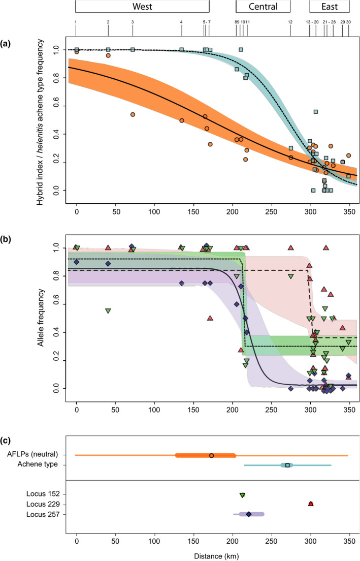
hzar results of geographical cline fitting across the helenitis–salisburgensis hybrid zone for five data sets, including: (a) the mean hybrid index (HI) values for all 30 populations (circles), based on the neutral AFLP data set (449 loci), and the relative frequencies of the helenitis‐achene type (pubescent) for 28 populations (squares), excluding nos. 13 and 21 (see Table 1); and (b) the fragment (“allele”) frequencies of three F _ST outlier loci, putatively under diversifying selection (fdist, bayescan), for all 30 populations (L152: inverted triangles; L229: triangles; L257: diamonds). Shading indicates 95% confidence intervals (CIs) around cline estimates. (c) Corresponding cline centres (symbols), CIs of cline centres (thick bars), and cline widths (thin bars). Numbers on top of (a) represent population numbers. Geographical distances (in km) are measured along the fitted transect, starting from the westernmost population no. 1. See Table 2 for hzar model parameter estimates [Colour figure can be viewed at wileyonlinelibrary.com]

3.6. Present and past climatic distribution predictions

The current maxent models for ssp. helenitis versus ssp. salisburgensis (Figure 6a vs. b) had very good versus excellent predictive power (mean AUC_train/test: 0.929/0.920 vs. 0.995/0.993), with low risk of model overfitting. Consequently, they adequately depicted the actual distribution of each taxon (defined as modelled suitability >0.5). For the West/Central European ssp. helenitis, particularly suitable climate conditions (≥0.85) presently occur in South Germany and along the entire central Northern Alps, with highest suitability (c. 1.0) in the west‐central part of the study transect (Figure 6a). Although this latter sector is suitable for ssp. salisburgensis as well, the most favourable conditions for this taxon presently occur further east (Salzburg area; Figure 6b). At the HCO (c. 6 ka BP), the European range of ssp. helenitis apparently fragmented into several disjunct areas (e.g., North Spain, Central/South France, South Germany), with suitable habitat covering only the west‐central sector (up to c. 170 km; Munich area; Figure 6c). For ssp. salisburgensis, however, both the central (“Munich”) and eastern (“Salzburg”) sectors would have provided suitable HCO conditions as well (Figure 6d), suggesting range overlap of both taxa in the central part of the transect at that time (see white‐dashed circles in Figure 6c,d). Finally, during the LGM (c. 22 ka BP), the Central European range of ssp. helenitis probably retracted to the west (e.g., West/Central France and adjoining, then‐exposed continental shelf sea areas), with suitable conditions closest to the transect found in the Rhone Valley/southwestern Pre‐Alps (see red arrow in Figure 6e) or, potentially, farther south of the Alps (Italy, West Balkans), but not along the transect. In striking contrast, for ssp. salisburgensis, the LGM model provided no evidence for suitable habitat along the central Northern Alps, or elsewhere (Figure 6f).

FIGURE 6.

Potential distributions of subspp. helenitis and salisburgensis in Europe and along the defined transect (black solid line) in the forelands of central Northern Alps at (a, b) the present (c. 1950–2000); (c, d) the mid‐Holocene Climate Optimum (HCO, c. 6 ka BP); and (e, f) the Last Glacial Maximum (LGM, c. 22 ka BP), with ice‐sheet limits derived from Ehlers et al. (2011). Ecological niche models were generated in maxent on the basis of 12 current bioclimatic variables and specimen records from GBIF and this study (see text). Predicted distribution probabilities (ranging from zero to one) are shown in each 2.5 arc‐minute pixel. Maps were generated using qgis 3.8 (QGIS Development Team, 2019). Note the potential range overlap of the two taxa in the central part of the transect at the HCO (c, d; white‐dashed circles), the presence of suitable LGM conditions for ssp. helenitis in the Rhone Valley/southwestern Pre‐Alps (e; red arrow), and the lack of suitable LGM habitats for ssp. salisburgensis along the transect, or elsewhere (f). M, Munich; S, Salzburg [Colour figure can be viewed at wileyonlinelibrary.com]

4. Discussion

The present AFLP survey of Tephroseris helenitis populations from the central North‐Alpine forelands identified nonadmixed (parental) individuals of subspp. helenitis and salisburgensis dominating, respectively, the westernmost and eastern parts of our c. 350 km long transect, with putative hybrid (admixed) individuals occurring in between (Figure 4a). Hence, this study system conforms to the notion of a “hybrid zone” where genetically distinct individuals of populations/taxa differing in one or more diagnostic traits (here: achene type) meet, mate, and produce hybrid offspring (Arnold, 1997). Collectively, our ENM, population genetic and cline analyses seem to indicate that this subspecies transition arose via primary differentiation (sensu Endler, 1977), following the species’ postglacial range expansion into the study area. Below we review the evidence for this hypothesis against predictions raised by alternative models of secondary contact.

4.1. ENM and population genetic evidence for west‐to‐east range expansion

Our palaeo‐niche models provided no evidence for a historically allopatric phase of the two subspecies of T. helenitis in the North‐Alpine forelands. During the LGM (c. 22 ka BP), suitable climate conditions probably existed for only ssp. helenitis in areas further west, including the Rhone Valley/southwestern Pre‐Alps (Figure 6e). By contrast, at this time, suitable habitat for ssp. salisburgensis was apparently absent along the transect, or elsewhere (Figure 6f). However, at the HCO (c. 6 ka BP), models for each subspecies indicate potential range overlap in the central part of the transect (see Figure 6c,d). It is feasible, therefore, that ssp. helenitis expanded postglacially from this geographically closest refugium into the present location of the transect by colonizing wet fens and grasslands that probably initiated soon after LGM climate amelioration in deglaciated areas of depression (ground/end moraines, lake basins) in the North‐Alpine forelands (c. 17–13 ka BP; Jäger et al., 2015; Rausch, 1975). Possibly, this south‐west to north‐east expansion was further assisted by increases in summer temperature and atmospheric moisture over the Alps during the early/mid‐Holocene (Mauri et al., 2015).

Clearly, this biogeographic scenario heavily relies on the assumption that the climate variables used for ENM modelling sufficiently represent conserved niche requirements of the taxa involved (Wielstra, 2019). It also probably suffers from various other issues commonly affecting these models (e.g., imperfect presence/absence records, residual spatial/temporal autocorrelation; Guélat & Kéry, 2016). Nonetheless, this range expansion scenario gains support by several lines of genetic evidence. First, we found a significant decrease of within‐population allelic rarity (DW) with longitude, i.e., along the presumed route of west‐to‐east colonization and possibly as a result of serial founder events (Hewitt, 1999). That estimates of PPF and H _E failed to register such a trend is not unexpected because these parameters are less sensitive to the loss of rare alleles in recently expanded/bottlenecked populations (Aguilar et al., 2008). Implicitly, neither diversity parameter was at maximum in the centre of the transect, as otherwise indicative of secondary contact (Gay et al., 2008). Second, our Φ _PT estimate of overall population differentiation in T. helenitis (0.154) is much lower than corresponding averages reported for other outcrossing (0.27) or wind‐dispersed (0.25) plant species (Nybom, 2004). As the studied populations are patchily distributed in a fragmented wet fen/grassland landscape (e.g., Stöhr, 2009; G. Pflugbeil, personal observation), it is unlikely that their shallow genetic divergence reflects high ongoing gene flow. Hence, their strong IBD pattern could be more a consequence of serial colonization (see above) rather than ongoing drift‐migration processes (Orsini et al., 2013). Finally, the spatial interpolation maps (Figure S1) confirmed a gradual allelic change from western (ssp. helenitis) to eastern (ssp. salisburgensis) ancestry. This is predicted for clines at (mostly) neutral loci produced by founder effects on the edge of a range expansion (Excoffier & Ray, 2008; Klopfstein et al., 2006).

4.2. Discordance across geographical cline patterns

Stable tension zones typically demonstrate (near) coincidental and concordant clines for diverse traits (genetic, morphological), whereby neutral loci should behave similarly as selected ones (Barton & Hewitt, 1985; Durrett et al., 2000). By contrast, our hzar analyses revealed significant noncoincidence in centre among the clines for neutral AFLPs, achene type, and outlier loci (L152/L257 vs. L229), plus significant nonconcordance in cline width (viz. selective strength) among at least some of those traits (Figure 5, Table 2). This pattern of discordance can be considered as necessary but not conclusive evidence for a primary hybrid zone subject to differential (exogenous) selection pressures (Endler, 1977; Futuyma, 2005). Yet, there are two additional cline features that appear to conflict with either stable or unstable tension zone models.

First, our estimated cline width for neutral AFLPs (c. 352 km), covering the entire transect, is much wider than expected for a tension zone at dispersal‐selection equilibrium. Using Endler’s (1977) neutral diffusion equation, and assuming dispersal distances of c. 0.24–0.54 km per generation, and c. 3000–9000 generations since hypothetical contact (see Section 2), we would expect such neutral clines to be just c. 33–129 km wide. Hence, a cline as broad as observed for our neutral AFLPs cannot be explained by free diffusion in a stable tension zone. This also implies that the underlying molecular markers are unlikely to be affected by some indirect selection (Gay et al., 2008; Scordato et al., 2017).

Second, rather than being a stable tension zone, it could be a dynamic and moving one (Buggs, 2007; Currat et al., 2008; Gay et al., 2008; Menon et al., 2019). This would be supported by the high incidence of western and central populations showing admixture with the “salisburgensis” gene pool II, and thus despite being nearly fixed for the pubescent (helenitis) achene type (Figure 4a,b). Under this scenario, asymmetric introgression of both neutral and advantageous alleles should have mainly occurred from a previously isolated (“native”) ssp. salisburgensis into an eastward‐expanding ssp. helenitis, due to lower densities of the latter at its wave front (Currat et al., 2008). In contrast, alleles of the invader will introgress the native only if “they are under very strong positive selection in that background” (cf. Currat et al., 2008; see also Barton & Bengtsson, 1986). As a consequence, in such a tension zone moving eastward, clines for individually selected traits/loci should have their centres mostly to the left (i.e., west) of the current hybrid zone boundary (as here defined by the neutral AFLP cline centre), i.e., being left behind as trails by the displaced taxon in the area where it was earlier replaced by the advancing one (Wielstra, 2019; see also Wielstra et al., 2017). This, however, is not observed, as our achene and outlier clines are consistently displaced to the right (i.e., east) (Figure 5, Table 2). Moreover, if the helenitis diagnostic trait (pubescent achenes) and respective diagnostic alleles at outlier loci, indeed, were under very strong positive selection, it would be puzzling that they had not progressed to fixation (see also Brumfield et al., 2001). Hence, while our genetic data cannot entirely rule out historical tension zone movement, we consider this scenario to be fairly unlikely, given the clinal patterns observed.

4.3. Primary hybrid zone formation and locus‐specific, climate‐driven selection

The preceding discussions leave primary hybrid zone formation, following postglacial range expansion, as the most plausible model to explain the genetic and phenotypic (achene) divergence across the helenitis–salisburgensis transition. Moreover, with further consideration of theory (e.g., Endler, 1977; Nei, 1987), data simulations (Currat et al., 2008; Klopfstein et al., 2006) and empirical cline studies (e.g., Antoniazza et al., 2010; Menon et al., 2019), we believe that the exceptionally broad neutral AFLP cline underlying this primary zone is largely a consequence of nonadaptive processes. According to this interpretation, stochastic drift, bottlenecks and founder events during the species’ eastward range expansion eventually resulted in two incompletely isolated gene pools (I vs. II; Figure 4a). Clearly, more detailed (e.g., genomic, simulation) studies would be required to investigate the effects of selection during this inferred range expansion, and especially whether new allelic variants (whether neutral, beneficial or, perhaps more likely, deleterious) might have spread or even increased in frequency towards the species’ easterly range edge (e.g., Barton, 2001; Gilbert et al., 2018; Lehe et al., 2012; Peischl et al., 2013; Peischl & Excoffier, 2015). Nonetheless, we find evidence for the presence of steep (and largely noncoincidental) clines for both outlier loci (step‐like) and achene type (sigmoid) staggered across the central‐eastern parts of the transect (Figure 5). Evidently, these clines are much narrower than predicted by the neutral (AFLP) data, suggesting that the differentiated alleles at these loci (or linked gene regions) as well as the two achene morphs are being maintained by selection (e.g., Barton & Hewitt, 1985; McKenzie et al., 2015). Nevertheless, it cannot be concluded from such cline shapes alone whether selection results from intrinsic lower fitness of hybrids (endogenous post‐mating barrier) or environment‐dependent pressures (exogenous selection; Gay et al., 2008).

While we have no data for testing the former hypothesis, the latter concurs with three lines of evidence. First, we found a pronounced west‐east climate gradient of increasingly wetter, cooler and temperature‐variable conditions across the sampled populations (Figure 3). Second, all three outlier loci, identified by both fdist and bayescan as undergoing diversifying selection, were significantly associated with various precipitation and temperature‐related variables (Table S4). Although their specific functions remain unclear, these loci (or closely linked loci) might be critical to local climate adaptation. Finally, based on our niche models, habitat suitability for ssp. helenitis is currently much higher in the west‐central (c. 1.0) than in the eastern part of the transect (c. 0.6–0.9; Figure 6a), and the latter was entirely unsuitable for this taxon c. 6000 years ago (Figure 6c). Together, these results suggest that T. helenitis experienced long‐term climatic constraints at the northern fringe of the Alps, causing diversifying selection at particular loci/gene regions along the wave of eastward advance.

4.4. Climate‐driven selection on achene indumentum?

Several previous studies have implied rainfall and/or temperature regimes in the clinal variation of species dimorphic for seed/diaspore morphology (e.g., Baskin & Baskin, 2014; Prentice, 1986), including cases of simple genetic basis (New & Herriot, 1981; Rollins, 1958). Moreover, inter‐ or intraspecific dimorphism for pubescent versus glabrous achenes is frequently observed in Tephroseris (Cufodontis, 1933) and other Asteraceae/Senecioneae (e.g., Andrés‐Sánchez et al., 2015; Le Roux et al., 2006). Diverse adaptive functions have also been proposed for the presence of achene hairs (trichomes), for instance, by aiding epizoic dispersal (via mucilage exudation upon wetting; Coleman et al., 2003) and/or mediating germination, especially at low water potential (e.g., via retarding water loss, increasing soil surface contact, and facilitating water diffusion; Kreitschitz, 2012; Roth, 1977). Together, this raises questions about the selective role of climatic constraints in driving the near fixation of the glabrous (or sparsely hairy) achene morph in the eastern core region of ssp. salisburgensis (Figures 3a and 5a).

Based on 28 populations, we found a highly significant negative (p < .001) relationship between the proportion of pubescent‐achene plants and among‐site variation in climate (PC1) space (Figure 3), suggesting that the variant with glabrous/sparsely hairy achenes could be more tolerant of higher precipitation and lower (winter) temperatures than the pubescent morph. In addition, all three outlier loci potentially under climate‐driven selection were also strongly associated with achene type (Table S4). However, given the noncoincidence in centre among the clines for achene type and these loci (Figure 5, Table 2), it is unlikely that they directly affect this phenotypic trait. Nonetheless, these locus‐trait associations reinforce the idea that the loss of achene pubescence in ssp. salisburgensis might also reflect a climate‐adaptive response. Although the specific function of this character state is unknown, it might convey a selective advantage (relative to the pubescent one) by mediating germination at higher water potential and lower temperatures (e.g., via facilitating the passage of oxygen to the embryo and its gas exchange with waterlogged soil; Setter & Belford, 1990; Werker, 1997). However, further experimental testing is required to obtain data on the ecophysiological and adaptive roles of this achene type variation and its genetic basis.

5. CONCLUSIONS

This study on Tephroseris helenitis adds to the vast hybrid zone literature, with past and current emphasis on secondary contact models, a rare example of hybrid zone formation caused by primary differentiation within a plant species, underlaid by historical range expansion. The clinal changes observed across this primary zone probably reflect (a) random/nonadaptive processes during the species’ postglacial, eastward expansion, and (b) exogenous, diversifying selection on particular loci, and possibly achene type, in response to a long‐term gradient in the direction of more stressful (e.g., wetter/cooler) climate conditions. As a result, only populations from the western‐ and easternmost parts of our transect are recognizable in genotype and (achene) phenotype as subspp. helenitis and salisburgensis, respectively. Future work should provide a thorough testing of the above hypotheses by integrating population genomic approaches with surveys of quantitative trait variation and experimental (e.g., crossing/reciprocal transplant/fitness) studies, also by including more western locations. Concomitantly, this study highlights the North‐Alpine forelands as a fruitful, but grossly understudied empirical avenue (but see Bresinsky, 1965) for unveiling neutral versus adaptive processes during past range expansions into relatively recent (i.e., deglaciated) environments that are probably conducive to the formation of primary hybrid zones.

AUTHOR CONTRIBUTIONS

A.T. and H.P.C. conceived the study. M.A. and H.P.C. wrote the paper with input from all authors. G.P. and A.T. conducted fieldwork and sample collection. G.P. and M.A. provided data generation and analyses.

Supporting information

Supplementary Material

Fig S1

Fig S2

Fig S3

DATA AVAILABILITY STATEMENT

The AFLP data matrix generated for this study is deposited in Dryad: https://doi.org/10.5061/dryad.2rbnzs7mr. Note, this matrix also includes information on achene type as known for 216 of the 233 genotyped individuals. There are no restrictions on data availability.

REFERENCES

- Abbott, R. J. (2017). Plant speciation across environmental gradients and the occurrence and nature of hybrid zones. Journal of Systematics and Evolution, 55, 238–258. [Google Scholar]
- Abbott, R. J. , Comes, H. P. , Goodwin, Z. A. , & Brennan, A. C. (2018). Hybridization and the detection of a hybrid zone between mesic and desert ragworts (Senecio) across an aridity gradient in the eastern Mediterranean. Plant Ecology and Diversity, 11, 1–15. [Google Scholar]
- Aguilar, R. , Quesada, M. , Ashworth, L. , Herrerias‐Diego, Y. , & Lobo, J. (2008). Genetic consequences of habitat fragmentation in plant populations: susceptible signals in plant traits and methodological approaches. Molecular Ecology, 17, 5177–5188. [DOI] [PubMed] [Google Scholar]
- Andrés‐Sánchez, S. , Galbany‐Casals, M. , Bergmeier, E. , Rico, E. , & Martínez‐Ortega, M. (2015). Systematic significance and evolutionary dynamics of the achene twin hairs in Filago (Asteraceae, Gnaphalieae) and related genera: Further evidence of morphological homoplasy. Plants Systematics and Evolution, 301, 1653–1668. [Google Scholar]
- Antoniazza, S. , Burri, R. , Fumagalli, L. , Goudet, J. , & Roulin, A. (2010). Local adaptation maintains clinal variation in melanin‐based coloration of European barn owls (Tyto alba). Evolution, 64, 1944–1954. [DOI] [PubMed] [Google Scholar]
- Arnold, M. L. (1997). Natural hybridization and evolution. Oxford University Press. [Google Scholar]
- Barton, N. H. (2001). Adaptation at the edge of a species range. In Silvertown J., & Antonovics J. (Eds.), Integrating ecology and evolution in a spatial context (pp. 365–392). Blackwell. [Google Scholar]
- Barton, N. , & Bengtsson, B. O. (1986). The barrier to genetic exchange between hybridising populations. Heredity, 56, 357–376. [DOI] [PubMed] [Google Scholar]
- Barton, N. H. , & Gale, K. S. (1993). Genetic analysis of hybrid zones. In Harrison R. G. (Ed.), Hybrid zones and the evolutionary process (pp. 13–42). Oxford University Press. [Google Scholar]
- Barton, N. H. , & Hewitt, G. M. (1985). Analysis of hybrid zones. Annual Review of Ecology and Systematics, 16, 113–148. [Google Scholar]
- Baskin, C. C. , & Baskin, J. M. (2014). Seeds: Ecology, biogeography, and evolution of dormancy and germination (2nd ed.). Academic Press. [Google Scholar]
- Basto, M. P. , Santos‐Reis, M. , Simões, L. , Grilo, C. , Cardoso, L. , Cortes, H. , Bruford, M. W. , & Fernandes, C. (2016). Assessing genetic structure in common but ecologically distinct carnivores: the stone marten and red fox. PLoS One, 11, e0145165. [DOI] [PMC free article] [PubMed] [Google Scholar]
- Bendiksby, M. , Tribsch, A. , Borgen, L. , Trávníček, P. , & Brysting, A. K. (2011). Allopolyploid origins of the Galeopsis tetraploids – Revisiting Müntzing’s classical textbook example using molecular tools. New Phytologist, 191, 1150–1167. [DOI] [PubMed] [Google Scholar]
- Bonin, A. , Ehrich, D. , & Manel, S. (2007). Statistical analysis of amplified fragment length polymorphism data: A toolbox for molecular ecologists and evolutionists. Molecular Ecology, 16, 3737–3758. [DOI] [PubMed] [Google Scholar]
- Brennan, A. C. , Bridle, J. R. , Wang, A. L. , Hiscock, S. J. , & Abbott, R. J. (2009). Adaptation and selection in the Senecio (Asteraceae) hybrid zone on Mount Etna, Sicily. New Phytologist, 183, 702–717. [DOI] [PubMed] [Google Scholar]
- Bresinsky, A. (1965). Zur Kenntnis des circum‐alpinen Florenelementes im Vorland nördlich der Alpen. Berichte der Bayerischen Botanischen Gesellschaft zur Erforschung der Heimischen Flora, 38, 5–67. [Google Scholar]
- Brumfield, R. T. , Jernigan, R. W. , McDonald, D. B. , & Braun, M. J. (2001). Evolutionary implications of divergent clines in an avian (Manacus: Aves) hybrid zone. Evolution, 55, 2070–2087. [DOI] [PubMed] [Google Scholar]
- Buchalski, M. R. , Sacks, B. N. , Gille, D. A. , Penedo, M. C. T. , Ernest, H. B. , Morrison, S. A. , & Boyce, W. M. (2016). Phylogeographic and population genetic structure of bighorn sheep (Ovis canadensis) in North American deserts. Journal of Mammalogy, 97, 823–838. [DOI] [PMC free article] [PubMed] [Google Scholar]
- Buggs, R. J. A. (2007). Empirical study of hybrid zone movement. Heredity, 99, 301–312. [DOI] [PubMed] [Google Scholar]
- Chater, A. O. , & Walters, S. M. (1976). Senecio L. In Tutin T. B., Burges N. A., Chater A. O., Edmondson J. R., Heywood V. H., Moore D. M., Valentine D. H., Walters S. M., & Webb D. A. (Eds.), Flora Europaea (Vol. 4, pp. 191–205). Cambridge University Press. [Google Scholar]
- Coleman, M. , Liston, A. , Kadereit, J. W. , & Abbott, R. J. (2003). Repeat intercontinental dispersal and Pleistocene speciation in disjunct Mediterranean and desert Senecio (Asteraceae). American Journal of Botany, 90, 1446–1454. [DOI] [PubMed] [Google Scholar]
- Coyne, J. A. , & Orr, H. A. (2004). Speciation. Sinauer Associates. [Google Scholar]
- Cufodontis, G. (1933). Kritische Revision von Senecio sectio Tephroseris . Feddes Repertorium Novarum Specierum Regni Vegetabilis, 70, 1–266. [Google Scholar]
- Cui, J.‐Y. , Miao, H. , Ding, L.‐H. , Wehner, T. C. , Liu, P.‐N. , Wang, Y. E. , Zhang, S.‐P. , & Gu, X.‐F. (2016). A new glabrous gene (csgl3) identified in trichome development in cucumber (Cucumis sativus L.). PLoS One, 11, e0148422. [DOI] [PMC free article] [PubMed] [Google Scholar]
- Currat, M. , Ruedi, M. , Petit, R. J. , & Excoffier, L. (2008). The hidden side of invasions: massive introgression by local genes. Evolution, 62, 1908–1920. [DOI] [PubMed] [Google Scholar]
- Derryberry, E. P. , Derryberry, G. E. , Maley, J. M. , & Brumfield, R. T. (2014). HZAR: Hybrid zone analysis using an R software package. Molecular Ecology Resources, 14, 652–663. [DOI] [PubMed] [Google Scholar]
- Durand, E. , Jay, F. , Gaggiotti, O. E. , & François, O. (2009). Spatial inference of admixture proportions and secondary contact zones. Molecular Biology and Evolution, 26, 1963–1973. [DOI] [PubMed] [Google Scholar]
- Durrett, R. , Buttel, L. , & Harrison, R. (2000). Spatial models for hybrid zones. Heredity, 84, 9–19. [DOI] [PubMed] [Google Scholar]
- Ehlers, J. , Gibbard, P. L. , & Hughes, P. D. (2011). Quaternary glaciation extent and chronology: A closer look. Developments in Quaternary Science (Vol. 15). Elsevier. [Google Scholar]
- Ehrich, D. (2006). Aflpdat: A collection of R functions for convenient handling of AFLP data. Molecular Ecology Notes, 6, 603–604. [Google Scholar]
- Endler, J. A. (1977). Geographic variation, speciation, and clines. Princeton University Press. [PubMed] [Google Scholar]
- Excoffier, L. , & Lischer, H. E. L. (2010). Arlequin suite ver 3.5: A new series of programs to perform population genetics analyses under Linux and Windows. Molecular Ecology Resources, 10, 564–567. [DOI] [PubMed] [Google Scholar]
- Excoffier, L. , & Ray, N. (2008). Surfing during population expansions promotes genetic revolutions and structuration. Trends in Ecology and Evolution, 23, 347–351. [DOI] [PubMed] [Google Scholar]
- Filatov, D. A. , Osborne, O. G. , & Papadopulos, A. S. T. (2016). Demographic history of speciation in a Senecio altitudinal hybrid zone on Mt Etna. Molecular Ecology, 25, 2467–2481. [DOI] [PubMed] [Google Scholar]
- Fischer, M. A. , Oswald, K. , & Adler, W. (2008). Exkursionsflora für Österreich, Liechtenstein und Südtirol (3rd ed.). Biologiezentrum der Oberösterreichischen Landesmuseen. [Google Scholar]
- Fois, M. , Cuena‐Lombraña, A. , Fenu, G. , & Bacchetta, G. (2018). Using species distribution models at local scale to guide the search of poorly known species: Review, methodology issues and future directions. Ecological Modelling, 385, 124–132. [Google Scholar]
- Foll, M. , & Gaggiotti, O. (2008). A genome‐scan method to identify selected loci appropriate for both dominant and codominant markers: A Bayesian perspective. Genetics, 180, 977–993. [DOI] [PMC free article] [PubMed] [Google Scholar]
- Futuyma, D. J. (2005). Evolution. Sinauer Associates. [Google Scholar]
- Gay, L. , Crochet, P. A. , Bell, D. A. , & Lenormand, T. (2008). Comparing clines on molecular and phenotypic traits in hybrid zones: A window on tension zone models. Evolution, 62, 2789–2806. [DOI] [PubMed] [Google Scholar]
- Gilbert, K. J. , Peischl, S. , & Excoffier, L. (2018). Mutation load dynamics during environmentally‐driven range shifts. PLoS Genetics, 14, e1007450. [DOI] [PMC free article] [PubMed] [Google Scholar]
- Gompert, Z. , & Buerkle, C. A. (2010). INTROGRESS: A software package for mapping components of isolation in hybrids. Molecular Ecology Notes, 10, 378–384. [DOI] [PubMed] [Google Scholar]
- Gompert, Z. , & Buerkle, C. A. (2016). What, if anything, are hybrids: Enduring truths and challenges associated with population structure and gene flow. Evolutionary Applications, 9, 909–923. [DOI] [PMC free article] [PubMed] [Google Scholar]
- Guélat, J. , & Kéry, M. (2016). Effects of spatial autocorrelation and imperfect detection on species distribution models. Methods in Ecology and Evolution, 9, 1614–1625. [Google Scholar]
- Hammer, O. , Harper, D. A. T. , & Ryan, P. D. (2001). PAST: Paleontological statistics software package for education and data analysis. Palaeontologia Electronica, 4, 9. [Google Scholar]
- Harrison, R. G. , & Larson, E. L. (2016). Heterogeneous genome divergence, differential introgression, and the origin and structure of hybrid zones. Molecular Ecology, 25, 2454–2466. [DOI] [PMC free article] [PubMed] [Google Scholar]
- Hewitt, G. M. (1999). Post‐glacial re‐colonization of European biota. Biological Journal of the Linnean Society, 68, 87–112. [Google Scholar]
- Hewitt, G. M. (2000). The genetic legacy of the Quaternary ice ages. Nature, 405, 907–913. [DOI] [PubMed] [Google Scholar]
- Hosmer, D. W. , & Lemeshow, S. (2000). Applied logistic regression. John Wiley and Sons Inc. [Google Scholar]
- Isotta, F. A. , Frei, C. , Weilguni, V. , Tadić, M. P. , Lassègues, P. , Rudolf, B. , Pavan, V. , Cacciamani, C. , Antolini, G. , Ratto, S. M. , Munari, M. , Micheletti, S. , Bonati, V. , Lussana, C. , Ronchi, C. , Panettieri, E. , Marigo, G. , Vertačnik, G. (2013). The climate of daily precipitation in the Alps: Development and analysis of a high‐ resolution grid dataset from pan‐Alpine rain‐gauge data. International Journal of Climatology, 34, 1657–1675. [Google Scholar]
- Jäger, H. , Achermann, M. , Waroszewski, J. , Kabała, C. , Malkiewicz, M. , Gärtner, H. , Dahms, D. , Krebs, R. , & Egli, M. (2015). Pre‐alpine mire sediments as a mirror of erosion, soil formation and landscape evolution during the last 45 ka. Catena, 128, 63–79. [Google Scholar]
- Jakobsson, M. , & Rosenberg, N. A. (2007). CLUMPP: A cluster matching and permutation program for dealing with label switching and multimodality in analysis of population structure. Bioinformatics, 23, 1801–1806. [DOI] [PubMed] [Google Scholar]
- Jaros, U. , Fischer, G. A. , Pallier, T. , & Comes, H. P. (2016). Spatial patterns of AFLP diversity in Bulbophyllum occultum (Orchidaceae) indicate long‐term refugial isolation in Madagascar and long‐distance colonization effects in La Réunion. Heredity, 116, 434–446. [DOI] [PMC free article] [PubMed] [Google Scholar]
- Johannesson, K. (2016). What can be learned from a snail. Evolutionary Applications, 9, 153–165. [DOI] [PMC free article] [PubMed] [Google Scholar]
- Klopfstein, S. , Currat, M. , & Excoffier, L. (2006). The fate of mutations surfing on the wave of a range expansion. Molecular Biology and Evolution, 23, 482–490. [DOI] [PubMed] [Google Scholar]
- Kreitschitz, A. (2012). Mucilage formation in selected taxa of the genus Artemisia L. (Asteraceae). Seed Science Research, 22, 177–189. [Google Scholar]
- Le Roux, J. J. , Wieczorek, A. M. , Ramadan, M. M. , & Tran, C. T. (2006). Resolving the native provenance of invasive fireweed (Senecio madagascariensis Poir.) in the Hawaiian Islands as inferred from phylogenetic analysis. Diversity and Distributions, 12, 694–702. [Google Scholar]
- Lehe, R. , Hallatschek, O. , & Peliti, L. (2012). The rate of beneficial mutations surfing on the wave of a range expansion. PLoS Computational Biology, 8, e1002447. [DOI] [PMC free article] [PubMed] [Google Scholar]
- Mauri, A. , Davis, B. A. S. , Collins, P. M. , & Kaplan, J. O. (2015). The climate of Europe during the Holocene: A gridded pollen‐based reconstruction and its multi‐proxy evaluation. Quaternary Science Reviews, 112, 109–127. [Google Scholar]
- McEntee, J. P. , Peñalba, J. V. , Werema, C. , Molungu, E. , Mbilinyi, M. , Moyer, D. , & Bowie, R. C. K. (2016). Social selection parapatry in an Afrotropical sunbird. Evolution, 70, 1307–1321. [DOI] [PubMed] [Google Scholar]
- McKenzie, J. L. , Dhillon, R. S. , & Schulte, P. M. (2015). Evidence for a bimodal distribution of hybrid indices in a hybrid zone with high admixture. Royal Society Open Science, 2, 150285. [DOI] [PMC free article] [PubMed] [Google Scholar]
- Menon, M. , Landguth, E. , Leal‐Saenz, A. , Bagley, J. C. , Schoettle, A. W. , Wehenkel, C. , & Eckert, A. J. (2019). Tracing the footprints of a moving hybrid zone under a demographic history of speciation with gene flow. Evolutionary Applications, 13, 1–15. [DOI] [PMC free article] [PubMed] [Google Scholar]
- Meusel, H. , & Jäger, E. J. (1992). Vergleichende Chorologie der Zentraleuropäischen Flora (Vol. 3). Gustav Fischer Verlag. [Google Scholar]
- Morales‐Rozo, A. , Tenorio, E. A. , Carling, M. D. , & Cadena, C. D. (2017). Origin and cross‐century dynamics of an avian hybrid zone. BMC Evolutionary Biology, 17, 257. [DOI] [PMC free article] [PubMed] [Google Scholar]
- Nei, M. (1987). Molecular evolutionary genetics. Columbia University Press. [Google Scholar]
- New, J. K. , & Herriot, J. C. (1981). Moisture for germination as a factor affecting the distribution of the seed coat morphs of Spergula arvensis L. Watsonia, 13, 323–324. [Google Scholar]
- Nybom, H. (2004). Comparison of different nuclear DNA markers for estimating intraspecific genetic diversity in plants. Molecular Ecology, 13, 1143–1155. [DOI] [PubMed] [Google Scholar]
- Orsini, L. , Vanoverbeke, J. , Swillen, I. , Mergeay, J. , & De Meester, L. (2013). Drivers of population genetic differentiation in the wild: Isolation by dispersal limitation, isolation by adaptation and isolation by colonization. Molecular Ecology, 22, 5983–5999. [DOI] [PubMed] [Google Scholar]
- Ostevik, K. L. , Moyers, B. T. , Owens, G. L. , & Rieseberg, L. H. (2012). Parallel ecological speciation in plants? International Journal of Ecology, 2012, e939862. [Google Scholar]
- Peakall, R. , & Smouse, P. E. (2012). GenALEx 6.5: Genetic analysis in Excel. Population genetic software for teaching and research – An update. Bioinformatics, 28, 2537–2539. [DOI] [PMC free article] [PubMed] [Google Scholar]
- Peischl, S. , Dupanloup, I. , Kirkpatrick, L. , & Excoffier, L. (2013). On the accumulation of deleterious mutations during range expansions. Molecular Ecology, 22, 5972–5982. [DOI] [PubMed] [Google Scholar]
- Peischl, S. , & Excoffier, L. (2015). Expansion load: Recessive mutations and the role of standing genetic variation. Molecular Ecology, 24, 20842084. [DOI] [PubMed] [Google Scholar]
- Phillips, S. J. , Anderson, R. P. , Dudík, M. , Schapire, R. E. , & Blair, M. E. (2017). Opening the black box: an open‐source release of Maxent. Ecography, 40, 887–893. [Google Scholar]
- Poelchau, M. F. , & Hamrick, J. L. (2012). Differential effects of landscape‐level environmental features on genetic structure in three codistributed tree species in Central America. Molecular Ecology, 21, 4970–4982. [DOI] [PubMed] [Google Scholar]
- Prentice, H. C. (1986). Climate and clinal variation in seed morphology of the white campion, Silene latifolia (Caryophyllaceae). Botanical Journal of the Linnean Society, 27, 179–189. [Google Scholar]
- QGIS Development Team (2019). QGIS Geographic Information System. Open Source Geospatial Foundation Project. Retrieved from http://qgis.osgeo.org. [Google Scholar]
- R Development Core Team (2017). R: A language and environment for statistical computing. R Foundation for Statistical Computing. [Google Scholar]
- Rausch, K. A. (1975). Untersuchungen zur spät‐ und nacheiszeitlichen Vegetationsgeschichte irn Gebiet des ehemaligen Inn‐Chiemseegletschers. Flora, 164, 235–282. [Google Scholar]
- Ripley, B. D. (1981). Spatial statistics. John Wiley and Sons Inc. [Google Scholar]
- Rollins, R. C. (1958). The genetic evaluation of a taxonomic character in Dithyrea (Cruciferae). Rhodora, 60, 145–152. [Google Scholar]
- Roth, I. (1977). Fruits of angiosperms. In Zimmermann W., Carlquist S., Ozenda P., & Wulff K. (Eds.), Encyclopedia of plant anatomy (Vol. 10, Part 1, pp. 1–675). Gebrüder Borntraeger. [Google Scholar]
- Rousset, F. (1997). Genetic differentiation and estimation of gene flow from F‐statistics under isolation by distance. Genetics, 145, 1219–1228. [DOI] [PMC free article] [PubMed] [Google Scholar]
- Schmickl, R. , & Koch, M. A. (2011). Arabidopsis hybrid speciation processes. Proceedings of the National Academy of Sciences USA, 108, 14192–14197. [DOI] [PMC free article] [PubMed] [Google Scholar]
- Scordato, E. S. C. , Wilkins, M. R. , Semenov, G. , Ruptsov, A. S. , Kane, N. C. , & Safran, R. J. (2017). Genomic variation across two barn swallow hybrid zones reveals traits associated with divergence in sympatry and allopatry. Molecular Ecology, 26, 5676–5691. [DOI] [PubMed] [Google Scholar]
- Setter, T. , & Belford, B. (1990). Waterlogging: How it reduces plant growth and how plants can overcome its effects. Journal of the Department of Agriculture, Western Australia, 31, 51–55. [Google Scholar]
- Stöhr, O. (2009). Tephroseris helenitis (L.) B.Nord. subsp. salisburgensis (Cufod.) B.Nord. (1978). In Rabitsch W., & Essl F. (Eds.), Endemiten: Kostbarkeiten in Österreichs Pflanzen‐ und Tierwelt (pp. 246–247). Naturwissenschaftlicher Verein für Kärnten und Umweltbundesamt GmbH. [Google Scholar]
- Thorpe, R. S. (1991). Clines and cause: Microgeographic variation in Tenerife Gecko (Tarentola delalandii). Systematic Zoology, 40, 172–187. [Google Scholar]
- Vasemägi, A. (2006). The adaptive hypothesis of clinal variation revisited: Single‐locus clines as a result of spatially restricted gene flow. Genetics, 173, 2411–2414. [DOI] [PMC free article] [PubMed] [Google Scholar]
- Vos, P. , Hogers, R. , Bleeker, M. , Reijans, M. , Lee, T. V. D. , Hornes, M. , Friters, A. , Pot, J. , Paleman, J. , Kuiper, M. , & Zabeau, M. (1995). AFLP: A new technique for DNA fingerprinting. Nucleic Acids Research, 23, 4407–4414. [DOI] [PMC free article] [PubMed] [Google Scholar]
- Warren, D. L. , Glor, R. E. , & Turelli, M. (2010). ENMTools: A toolbox for comparative studies of environmental niche models. Ecography, 33, 607–611. [Google Scholar]
- Werker, E. (1997). Seed anatomy. In Carlquist S., Cutler D. F., Fink S., Ozenda P., Roth I., & Ziegler H. (Eds.), Encyclopedia of plant anatomy (Vol. 10, Part 3, pp. 1–424). Gebrüder Borntraeger. [Google Scholar]
- Wielstra, B. (2019). Historical hybrid zone movement: More pervasive than appreciated. Journal of Biogeography, 46, 1300–1305. [Google Scholar]
- Wielstra, B. , Burke, T. , Butlin, R. K. , Avcı, A. , Üzüm, N. , Bozkurt, E. , Olgun, K. , & Arntzen, J. W. (2017). A genomic footprint of hybrid zone movement in crested newts. Evolution Letters, 1, 93–101. [DOI] [PMC free article] [PubMed] [Google Scholar]
Associated Data
This section collects any data citations, data availability statements, or supplementary materials included in this article.
Supplementary Materials