Three-class brain tumor classification using deep dense inception residual network

Abstract

Three-class brain tumor classification becomes a contemporary research task due to the distinct characteristics of tumors. The existing proposals employ deep neural networks for the three-class classification. However, achieving high accuracy is still an endless challenge in brain image classification. We have proposed a deep dense inception residual network for three-class brain tumor classification. We have customized the output layer of Inception ResNet v2 with a deep dense network and a softmax layer. The deep dense network has improved the classification accuracy of the proposed model. The proposed model has been evaluated using key performance metrics on a publicly available brain tumor image dataset having 3064 images. Our proposed model outperforms the existing model with a mean accuracy of 99.69%. Further, similar performance has been obtained on noisy data.

Introduction

Medical image processing has enriched with a wide variety of applications and some of them are as follows. Chauhan and Choi (2018) have reported brain digital image denoising algorithms and their performance analysis. Fuzzy logic and a convolutional autoencoder-based approach have been presented by Chauhan and Choi (2019) for denoising of biomedical images. Image classification is a widely used task in computer vision applications. Varela-Santos and Melin (2020) have extracted Haralick’s texture features and have performed pneumonia detection using a neural network. Varela-Santos and Melin (2021) have proposed convolutional neural network for COVID-19 classification. Poma et al. (2020) have employed fuzzy gravitational search to optimize the CNN model for image classification.

Brain cancer is one of the most common and the major causes that increase mortality among children and adults in the world (El-Sayed et al. 2014). Thus, brain image processing receives great attention in medical image processing. Magnetic resonance (MR) and computed tomography (CT) are the commonly used imaging techniques for brain tumor diagnosis. MR imaging renders more detailed pictures of the brain than CT scans. Hence, it becomes an essential tool for neurologists to perform brain tumor diagnosis (Chetih et al. 2018). Nowadays, there is a rapid increase in brain tumor cases. Manual inspection of such a high-scale tumor detection from MR images is a time-consuming process [12]. Thus, researchers have been motivated for automation of brain tumor diagnosis. Computer-aided diagnosis decreases the diagnosis time and allows for early-stage brain tumor detection (El-Sayed et al. 2014). Moreover, the early-stage diagnosis of the tumor plays a significant role in the improvement of treatment outcome and allows to increase patient survival (Abd-Ellah et al. 2019). Thus, brain tumor image classification has evolved as an intense research area for brain tumor diagnosis. In general, brain tumor image classification has been segregated into two types as binary and multi-class. Binary classification is popularly known as brain pathology detection that mainly classifies the given brain image as abnormal or normal. Numerous proposals can be observed in pathological brain detection. A deep wavelet autoencoder-based network has proposed by Kumar Mallick et al. (2019) for cancer detection, and AlexNet with transfer learning has utilized by Lu et al. (2019). Nayak et al. (2018) have employed fast curvelet entropy features for pathology detection. Kaur et al. (2018) have implemented fisher criteria and parameter-free BAT optimization algorithm, and Jude Hemanth (2019) has used a modified genetic algorithm for abnormal brain detection. Though binary classification performs pathology of the brain, it fails to detect the type of tumor. There are three common brain tumor types and the details of the tumors are as follows.

1. Meningioma tumor generally forms meninges under the skull.

2. Glioma tumor begins in glial cells and able to spread over white matter.

3. Pituitary tumor mostly affects in or around the pituitary gland of the brain.

Pituitary and meningioma tumors depict homogeneous intensities in MR images. Glioma tumor shows heterogeneous intensities and spread over the glial cells of the brain. Moreover, other properties such as location, shape, and size of these tumors vary from tumor to tumor. Thus, multi-class brain tumor classification became a contemporary research task in brain image classification. The multi-class brain tumor classification detects the type of tumor in addition to brain pathology. Tumor-type detection is challenging for the computer-aided diagnosis system as each tumor exhibit distinct properties such as intensity, location, size, and shape. Subudhi et al. (2019) have been developed an automatic decision system to detect ischemic stroke using a diffusion-weighted image sequence of MR images. An expectation–maximization algorithm has been used for segmentation. Fractional-order particle swarm optimization technique has been applied to the extracted segments for better classification accuracy. An automated method based on a deep extreme learning machine (ELM) has been presented by Nayak et al. (2018) for multi-class classification of the pathological brain. It is a multi-layer architecture stacked with ELM-based autoencoders. The system uses a deep learning model with a leaky rectified linear unit (ReLU) function for feature mapping. These models have been evaluated on small datasets and some of them are private datasets. In 2016, Cheng et al. (2016) have presented a content-based image retrieval framework for three-class brain tumor classification. Authors have published a brain tumor dataset of 3064 T1-weighted MR images. This dataset contains three common brain tumor types namely meningioma, glioma, and pituitary. Researchers have started working in this direction and hence three-class brain tumor classification has become a contemporary task.

Rest of the paper has organized as follows; Sect. 2 elaborates the literature review. Section 3 describes the proposed deep dense inception network model. Experimental results are discussed in Sect. 4 and the conclusion is presented in Sect. 5.

Literature review

In this section, we have provided the details of state-of-art models and Table 1 lists a summary of the review. A hybrid feature extraction method has been presented by Gumaei et al. (2019) for accurate brain tumor classification. Authors have extracted feature vector using normalized GIST descriptors and principal component analysis. Finally, a regularized extreme learning machine has been used for brain tumor image classification. Anaraki et al. (2019) have presented CNN using a genetic algorithm for brain tumor image classification. It consists of six convolutional and max-pooling layers with one fully connected layer. These models have used traditional neural networks and achieved an accuracy of 94%.

Table 1.

Summary of the existing three-class brain tumor classification models

References	Year	Dataset	Accuracy
Gumaei et al. (2019)	2019	BTDS	94.23
Anaraki et al. (2019)	2019	BTDS	94.20
Sajjad et al. (2019)	2018	BTDS	94.58
Swati et al. (2019)	2019	BTDS	94.82
Deepak and Ameer (2019)	2019	BTDS	97.10

A deep CNN with data augmentation has been devised by Sajjad et al. (2019) for multi-grade tumor classification. The pre-trained convolutional neural network (CNN) model is fine-tuned for classification. Similarly, Swati et al. (2019) have been designed an approach for the brain tumor image classification using fine-tuning of transfer learning. These deep transfer learning approaches have reported a small improvement in Accuracy. On the other hand, Deepak and Ameer (2019) have proposed deep transfer learning and support vector machine (SVM) for three-class classification. Authors have utilized a pre-trained GoogleNet to extract features from brain MR images. Then, the SVM classifier has employed for classification and achieved 97% accuracy.

In brain tumor image classification, achieving better classification accuracy is a challenging task. Thus, we have worked in a similar direction to design an efficient model for better accuracy. A deep dense inception network has been designed for three-class classification. The proposed model takes advantage of three dense layers to attain high performance. Further, the dropout technique has been used to avoid model overfitting.

Methodology

A deep convolutional neural network is a proficient tool for image classification (Kumar et al. 2021). VGGNet and Inception network are some of the popular deep networks. Vanishing gradients and high computational cost are the major demerits of deep learning models. VGGNet incurs high computational cost due to the huge number of trainable parameters (Simonyan and Zisserman 2014). Inception network reduced the computational time using factorized convolutions (Szegedy et al. 2014). Similarly, the residual network handles the vanishing gradients problem using skip connections (He et al. 2015). Szegedy et al. (2016) have devised an inception residual network to achieve better accuracy. Inception ResNet takes advantage of inception modules and residual connections. Thus, the proposed model has designed using Inception ResNet v2 for three-class brain tumor classification.

Basic inception block

Convolution is the dominant operation in a convolutional neural network. In general, convolution operations with larger spatial filters incurs to high computational cost. Inception module is one significant solution to reduce this cost. Inception module reduces the cost using optimal local sparse structures (Venkateswarlu et al. 2020). The inception block mainly designs a layer-by-layer construction using layer correlation statistics analysis. Filter banks are generated from clusters of highly correlated layers. Final results can be obtained from the concatenation of huge filter banks from a single region. These filter banks lead to patch alignment issues and are resolved using restricted filter sizes such as 1 $\times$ 1, 3 $\times$ 3, and 5 $\times$ 5. However, 1 $\times$ 1 convolution is performed to compute reductions before 3 $\times$ 3 and 5 $\times$ 5 convolutions. Thus, the inception block performs two steps for the generation of filter banks as follows.

1. Visual information processing at various scales from the same region.

2. Aggregation of abstract features from different scales simultaneously.

Consider the inception block with dimension reductions as shown in Fig. 1. Given input is passed through four simultaneous convolution paths with three scaled convolutions and one pooling. The first path takes 1 $\times$ 1 followed by 5 $\times$ 5 convolutions and the second path uses 1 $\times$ 1 followed by 3 $\times$ 3 convolutions. On the other hand, the third path takes pooling followed by 1 $\times$ 1 convolution, and the fourth path uses only 1 $\times$ 1 convolution. The output of the inception block is produced by the concatenation of the four filtered outputs coming from the above four convolution paths. This leads to high spatial filtering with layer correlations.

Fig. 1.

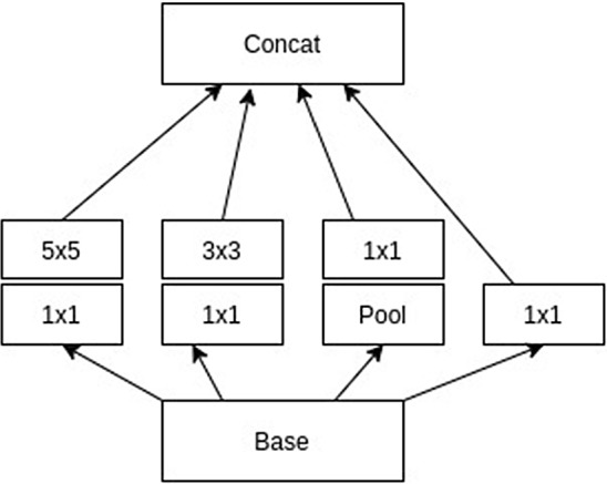
Basic inception block

Inception residual network

Inception residual network introduces the concept of residual connections for inception blocks. This network significantly improves recognition performance with three types of blocks as follows.

1. Stem block It is the initial block that accepts given input and performs three 3 $\times$ 3 convolutions. Then, the final stem block output is produced with three inception blocks. The first and third inception blocks consist of two paths with 3 $\times$ 3 convolutions and max-pooling. Similarly, the second block also includes two paths with 1 $\times$ 1 and 3 $\times$ 3 convolutions. However, one path of the second block uses 7 $\times$ 1 followed by 1 $\times$ 7 before 3 $\times$ 3 convolution.

2. Inception ResNet block Residual connections are included for inception blocks to avoid vanishing gradients. Inception ResNet v2 utilizes three types of Inception ResNet blocks. Inception ResNet-A block consists of three paths with 1 $\times$ 1 and 3 $\times$ 3 convolutions. Inception ResNet-B and Inception ResNet-C blocks consist of two paths. Though these blocks have identical convolutions, there is a change in convolution filter sizes.

3. Reduction block It uses pooling along with convolution paths for feature reduction. Reduction-A block consists of one max-pooling and two convolution paths. Reduction-B block consists of three convolution paths in addition to max-pooling.

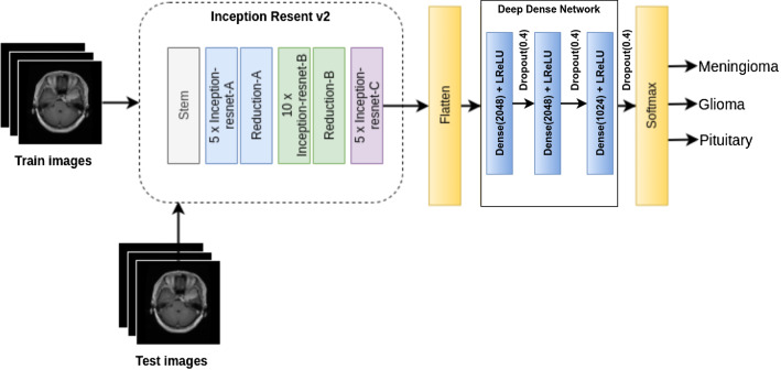
Inception ResNet v2 is a costlier hybrid inception network that achieves higher performance. It is a deep network that combines one stem block, five Inception ResNet-A, ten Inception ResNet-B, five Inception ResNet-C, one Reduction-A, and one Reduction-B block. The arrangement of these blocks can be visualized from Fig. 2.

Fig. 2.

Architecture of proposed DDIRNet model

Proposed deep dense inception ResNet

This section describes steps for the implementation of the proposed model from the basic inception residual network (IRNet). Original IRNet is intended for a thousand class classification and successful in the Imagenet challenge. We have customized the output layer as our objective is three-class classification. In addition to that, we have introduced a deep dense network before the softmax layer. This deep dense network consists of three dense layers. The first two dense layers consist of 2048 neurons while the third dense layer contains 1024 neurons. Each dense layer is associated with a leaky regularized linear unit (ReLU) and a dropout layer. We have employed the dropout technique to avoid overfitting. Steps for the design of a proposed deep dense inception network (DDIRNet) are as follows.

1. Initially, we have considered IRNet v2 without output layers and accepts (256, 256, 3) size image as input. It generates (6, 6, 1536) feature map before the output layer.

2. Above multi-dimensional feature map is flattened to generate a one-dimensional vector having 55,296 features.

3. Deep dense network accepts above one-dimensional feature vector and produces one-dimensional vector having 1024 features.

4. Finally, a softmax layer with three neurons has included for three-class classification as shown in Fig. 2.

The proposed model is referred to as deep dense inception ResNet (DDIRNet) as it uses inception ResNet and deep dense network. These additional dense layers significantly improve classification performance. The proposed model has initialized with Imagenet weights and we have disabled the parameters learning to reduce training time. However, the proposed model has allowed learning parameters of the three dense layers. In general, a regularized linear unit (ReLU) is the commonly used activation for dense layers due to its simplicity. However, the negative side of the ReLU activation becomes zeros. Thus, we have integrated leaky ReLU with each dense layer.

$$\begin{array}{c}\hfill \begin{array}{ccc}\psi (z)& =z\hfill & z\ge 0\hfill \\ & =\alpha .z\hfill & z<0.\hfill \end{array}\end{array}$$ 1

Leaky ReLU allows a small negative side as represented by Eq. 1. We have utilized leaky ReLU activation with $\alpha =0.2$ for each dense layer to preserve a controlled negative portion. Model overfitting is another problem in deep learning due to the huge number of features. A dropout technique removes randomly selected neurons to control model overfitting. Thus, the proposed model has devised the dropout value of 0.2 after each dense layer.

Results and discussion

This section presents the performance analysis of proposed model and state-of-art models with various key metrics. Most of the state-of-art models have analyzed their performance using a publicly available brain tumor dataset published by Cheng et al. (2016). Thus, we also have considered the same dataset for performance evaluation.

Experimental setup

In this section, we have provided an experimental setup along with model hyperparameters. Our proposed model has simulated using Python and Tensorflow. Adam is one of the time-efficient optimizer for deep networks. Thus, we have devised the Adam optimizer with an initial learning rate of 0.0001 for the compilation of the proposed model. We have considered a batch size of 50 and executed for 5 epochs to train the proposed model. Table 2 lists out all hyperparameters used while training the proposed model.

Table 2.

Hyperparameter setup of the proposed model

Hyperparameter	Value
Number of epochs	5
Batch size	50
Optimizer	Adam
Initial learning rate	0.0001

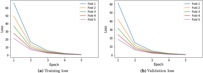
We have conducted experiments on Intel Xeon processor with 32 GB RAM. Further, we have analyzed our proposed model using fivefold cross-validation. The entire dataset is divided into two sets namely the train set and test set. In each fold, 75% of the dataset is used as a train and validation set, and the remaining 25% is used to test the model. The performance of the proposed model is computed on the test set and the mean performance is computed after fivefold. Figure 3a, b visualizes the training and validation loss over the fivefold cross-validation of the proposed model with 75% train size. The proposed model has disabled the learning of basic IRNet parameters and hence it produces high training and validation loss in the early epochs. The proposed model exhibits fast learning due to three dense layers and cross-entropy loss. The parameters of these dense layers are learned in each epoch and adapt the features of the brain tumors. It drives the model for a consistent decrease in both training and validation losses. The proposed model converges and attains optimal loss within five epochs. An optimal error of 0.5 has been recorded by the proposed model with optimal performance at the end of the fifth epoch.

Fig. 3.

Training and validation loss of proposed model

Results analysis of proposed model

In this section, we have presented the performance of proposed deep dense inception residual network (DDIRNet) model with key metrics. Four commonly used performance metrics such as accuracy, precision, recall, and F1-score have been considered to analyze the proposed model. “Accuracy is the sum of true positive and true negative samples divided by the total number of samples.” “Precision represents the percentage of relevant classification results.” “Recall refers to the percentage of total relevant results correctly classified by the model.” “F1-score is a measure of test accuracy that considers a harmonic average of both precision and recall.”

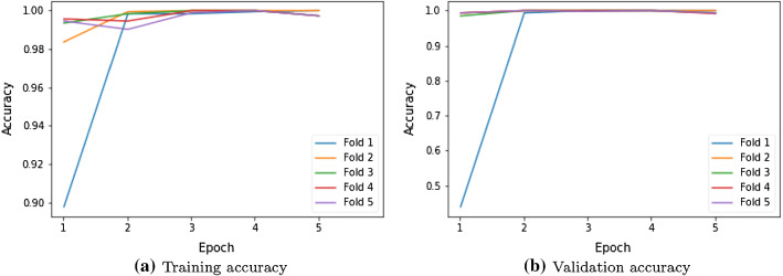
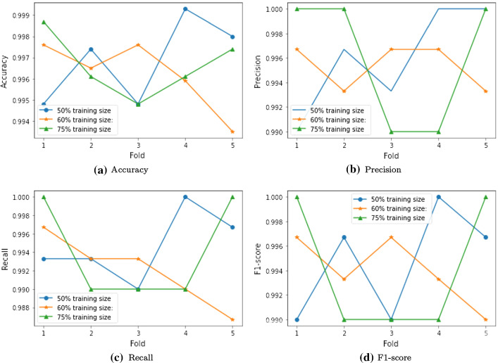
Figure 4a visualizes training accuracy over fivefold cross-validation. In fold-1, our proposed model achieves 90% of training accuracy in the first epoch while it attains around 98% in subsequent epochs. From the second fold onward, proposed model achieves a consistent training accuracy of 99%. Similarly, Fig. 4b depicts validation accuracy over fivefold cross-validation. In fold-1, the proposed model achieves 48% of validation accuracy in the first epoch while it attains around 98% in subsequent epochs. From the second fold onward, proposed model achieves a consistent validation accuracy of 99%. These figures reveal that our proposed model achieves maximum efficiency within five epochs. Three dense layers devised in the proposed model causes enhanced learning for better accuracy. In general, the training size influences the efficiency of deep learning models. If training size increases, then the model is trained with more samples and achieves better accuracy. Thus, we have analyzed the performance of the proposed model with various training sizes such as 50%, 60%, and 75% of the 3064 size dataset. Metric-wise analysis of the proposed model is as follows.

• Accuracy Figure 5a shows the accuracy of the proposed model with various training sizes. The proposed model achieves an accuracy of 99.5% (minimum) and 99.9% (maximum) with 50% training size. With 60% training size, it attains an accuracy of 99.3% (minimum) and 99.8% (maximum). It records the accuracy of 99.5% (minimum) and 99.9% (maximum) with 75% training size.

• Precision Figure 5b visualizes precision of the proposed model with various training sizes. The proposed model achieves a precision of 99.0% (minimum) and 100.0% (maximum) with 50% training size. With 60% training size, it attains a precision of 99.3% (minimum) and 99.7% (maximum). It records the precision of 99.0% (minimum) and 100.0% (maximum) with 75% training size.

• Recall Figure 5c depicts the recall of the proposed model with various training sizes. The proposed model achieves a recall of 99.0% (minimum) and 100.0% (maximum) with 50% training size. With 60% training size, it attains a recall of 98.7% (minimum) and 99.7% (maximum). It records a recall of 99.0% (minimum) and 100.0% (maximum) with 75% training size.

• F1-score Figure 5d shows F1-score of the proposed model with various training sizes. The proposed model exhibits similar performance as precision.

These figures prove that the proposed model attains a mean performance of 99% in all considered metrics. Table 3 lists out the mean performance of the proposed model with different training sizes. The proposed model achieves similar performance in all cases while it exhibits the best results with a 50% training size. The proposed model records 99.6% of classification accuracy, 99.6% of precision, 99.4% of recall, and 99.4% of F1-score. It shows that the proposed model exhibits consistent results even with different training sizes.

Fig. 4.

Training and validation accuracy of proposed model

Fig. 5.

Performance analysis of the proposed model with various training sizes

Table 3.

Performance of proposed model with different training sizes

Training size (%)	Accuracy	Precision	Recall	F1-score
50	99.69	99.60	99.47	99.47
60	99.62	99.53	99.20	99.40
75	99.66	99.60	99.40	99.40

We have analyzed the confusion matrix as it captures tumor-wise classification results. Table 4 lists out confusion matrix after fifth fold. This table shows that all tumor images of meningioma and pituitary have been classified correctly. However, only two glioma tumor images have been wrongly classified as pituitary. Thus, the accuracy of classification can be computed as $\frac{764}{766}\ast 100$ = 99.74%.

Table 4.

Confusion matrix of proposed model in fold-5

Actual	Predicted
	Meningioma	Glioma	Pituitary	Acc. %
Meningioma	409	0	0	99.74
Glioma	0	120	2
Pituitary	0	0	235

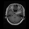
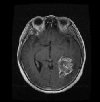
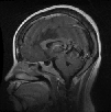
Table 5 depicts the best-case and worst-case performance of the proposed model. The first three columns represent the correct prediction of three classes of the dataset. The fourth column visualizes the wrong prediction of glioma tumor as pituitary. In addition to this, we also have evaluated the performance of proposed model on noisy image data. Blur noise is a frequently occurring noise in MR images. Thus, we have used Gaussian noise having different kernel sizes such as 9 $\times$ 9 and 5 $\times$ 5. Table 6 lists out the accuracy of proposed model on noisy image data. These results reveal that the proposed model exhibits similar accuracy of 99% on noisy image data.

Table 5.

Best- and worst-case performance of proposed model

Actual class	1	2	3	2
Predicted class	1	2	3	3

Table 6.

Performance of proposed model on noisy data

Fold	Accuracy
	9 $\times$ 9 kernel	5 $\times$ 5 kernel
1	99.59	99.43
2	99.76	99.59
3	99.76	99.76
4	99.51	99.10
5	99.18	99.51
Mean	99.56	99.48

Comparison with pre-trained models

Transfer learning has been established as one of the proven techniques for computer vision tasks especially image classification. In this approach, pre-trained models are again trained with domain-specific data to improve the performance. We have considered four popular pre-trained image classification models such as MobileNet, Res Net50, EfficientNet, GoogleNet, and Inception ResNet for the evaluation. Table 7 compares the accuracy of the proposed model with pre-trained models. This table shows that the proposed model outperforms the existing models as it employs three dense layers for higher-dimensional feature enhancement.

Table 7.

Comparison with pre-trained models

Model	Accuracy
MobileNet	97.19
ResNet50	93.60
EfficientNetb0	97.32
GoogleNet	97.91
Inception ResNet	97.03
DDIRNet	99.69

Comparison with state-of-the-art schemes

We have compared the accuracy of our proposed model with its competitive models such as Gumaei et al. (2019), Anaraki et al. (2019), Sajjad et al. (2019), Swati et al. (2019), and Deepak and Ameer (2019). It is observed that accuracy is the primary measure used to compare classification results. Thus, we have considered the mean accuracy for the quantitative analysis. Table 8 lists out the comparison accuracy of the proposed model with its competitive methods. This table reveals that the proposed model outperforms the existing models with 99.66% accuracy. Further, our model has achieved 2% improvement than Deepak and Ameer (2019) and 5% improvement than the existing models.

Table 8.

Comparison of accuracy with state-of-the-art models

References	Approach	Accuracy
Anaraki et al. (2019)	CNN + genetic algorithm	94.20
Gumaei et al. (2019)	Regularized extreme learning machine	94.23
Sajjad et al. (2019)	VGG19 + extensive data augmentation	94.58
Swati et al. (2019)	VGG19 + fine-tuning	94.82
Deepak and Ameer (2019)	GoogleNet + transfer learning	97.10
DDIRNet	Deep dense inception residual network	99.69

Discussion

An inception residual network-based network has been proposed for three-class brain tumor classification. The performance of the proposed model has been analyzed on a publicly available brain tumor dataset. The proposed model can automatically learn high-level abstractions from the input images directly. The results indicate that the proposed model has achieved better classification accuracy. The proposed model exhibits several advantages as compared to state-of-the-art models.

1. Inception residual network devised in the proposed model controls the vanishing gradient problem.

2. Three dense layers associated with the output layer have improved the performance of the proposed model.

3. Leaky ReLU activation has been used to avoid the dying ReLU problem.

4. It devises the dropout technique to reduce model overfitting.

5. It exhibits similar performance on noisy image data.

Conclusions

Deep neural networks became popular solutions for image classification. We have adapted IRNet v2 and proposed a deep dense inception residual network for three-class brain tumor classification. The proposed model has devised three dense layers along with a softmax layer as the output layer. These dense layers incorporate the features of the brain tumors while parameters of IRNet are initialized with Imagenet weights. The proposed model exhibits fast learning due to the use of Adam optimizer and dropout avoids the model overfitting problems. The commonly used brain tumor dataset with 3064 T1-weighted images has been considered for performance evaluation. Our proposed model outperforms the existing models with 99.69% accuracy. Further, the proposed model exhibits similar performance on noisy image data. Our future work focuses on reducing the number of parameters and computational time for the proposed model without compromising performance.

Declarations

Conflict of interest

The authors declare that there is no conflict of interest regarding the publication of this paper.

Ethical approval

This article does not contain any studies with human participants or animals performed by any of the authors.

Informed consent

Informed consent was obtained from all individual participants included in the study.

References

- Abd-Ellah MK, Awad AI, Khalaf AA, Hamed HF. A review on brain tumor diagnosis from MRI images: practical implications, key achievements, and lessons learned. Magn Reson Imaging. 2019;61:300–318. doi: 10.1016/j.mri.2019.05.028. [DOI] [PubMed] [Google Scholar]
- Anaraki AK, Ayati M, Kazemi F. Magnetic resonance imaging-based brain tumor grades classification and grading via convolutional neural networks and genetic algorithms. Biocybern Biomed Eng. 2019;39(1):63–74. doi: 10.1016/j.bbe.2018.10.004. [DOI] [Google Scholar]
- Chauhan N, Choi BJ. Performance analysis of denoising algorithms for human brain image. Int J Fuzzy Logic Intell Syst. 2018;18(3):175–181. doi: 10.5391/IJFIS.2018.18.3.175. [DOI] [Google Scholar]
- Chauhan N, Choi BJ. Denoising approaches using fuzzy logic and convolutional autoencoders for human brain MRI image. Int J Fuzzy Logic Intell Syst. 2019;19(3):135–139. doi: 10.5391/IJFIS.2019.19.3.135. [DOI] [Google Scholar]
- Cheng J, Yang W, Huang M, Huang W, Jiang J, Zhou Y. Retrieval of brain tumors by adaptive spatial pooling and fisher vector representation. PLoS ONE. 2016;11(6):e0157112. doi: 10.1371/journal.pone.0157112. [DOI] [PMC free article] [PubMed] [Google Scholar]
- Chetih N, Messali Z, Serir A, Ramou N. Robust fuzzy c-means clustering algorithm using non-parametric Bayesian estimation in wavelet transform domain for noisy MR brain image segmentation. IET Image Process. 2018;12(5):652–660. doi: 10.1049/iet-ipr.2017.0399. [DOI] [Google Scholar]
- Deepak S, Ameer P. Brain tumor classification using deep CNN features via transfer learning. Comput Biol Med. 2019;111:103345. doi: 10.1016/j.compbiomed.2019.103345. [DOI] [PubMed] [Google Scholar]
- El-Sayed A, El-Dahshan Mohsen HM, Revett K, Salem ABM. Computer-aided diagnosis of human brain tumor through MRI: a survey and a new algorithm. Expert Syst Appl. 2014;41(11):5526–5545. doi: 10.1016/j.eswa.2014.01.021. [DOI] [Google Scholar]
- Gumaei A, Hassan MM, Hassan MR, Alelaiwi A, Fortino G. A hybrid feature extraction method with regularized extreme learning machine for brain tumor classification. IEEE Access. 2019;7:36266–36273. doi: 10.1109/ACCESS.2019.2904145. [DOI] [Google Scholar]
- He K, Zhang X, Ren S, Sun J (2015) Deep residual learning for image recognition
- Jude Hemanth DJA Modified genetic algorithm approaches for classification of abnormal magnetic resonance brain tumour images. Appl Soft Comput. 2019;75:21–28. doi: 10.1016/j.asoc.2018.10.054. [DOI] [Google Scholar]
- Kakarla J, Isunuri BV, Doppalapudi KS, Bylapudi KSR (2021) Three-class classification of brain magnetic resonance images using average-pooling convolutional neural network. Int J Imaging Syst Technol
- Kaur T, Saini BS, Gupta S. An optimal spectroscopic feature fusion strategy for MR brain tumor classification using fisher criteria and parameter-free bat optimization algorithm. Biocybern Biomed Eng. 2018;38(2):409–424. doi: 10.1016/j.bbe.2018.02.008. [DOI] [Google Scholar]
- Kumar RL, Kakarla J, Isunuri BV, Singh M (2021) Multi-class brain tumor classification using residual network and global average pooling. Multimed Tools Appl 1–10 (2021)
- Kumar Mallick P, Ryu SH, Satapathy SK, Mishra S, Nguyen GN, Tiwari P. Brain MRI image classification for cancer detection using deep wavelet autoencoder-based deep neural network. IEEE Access. 2019;7:46278–46287. doi: 10.1109/ACCESS.2019.2902252. [DOI] [Google Scholar]
- Lu S, Lu Z, Zhang YD (2019) Pathological brain detection based on alexnet and transfer learning. J Comput Sci 30:41–47
- Nayak DR, Dash R, Chang X, Majhi B, Bakshi S. Automated diagnosis of pathological brain using fast curvelet entropy features. IEEE Trans Sustain Comput. 2018;5(3):416–427. doi: 10.1109/TSUSC.2018.2883822. [DOI] [Google Scholar]
- Poma Y, Melin P, González CI, Martinez GE (2020) Optimal recognition model based on convolutional neural networks and fuzzy gravitational search algorithm method. In: Hybrid intelligent systems in control, pattern recognition and medicine. Springer, pp 71–81
- Sajjad M, Khan S, Muhammad K, Wu W, Ullah A, Baik SW. Multi-grade brain tumor classification using deep CNN with extensive data augmentation. J Comput Sci. 2019;30:174–182. doi: 10.1016/j.jocs.2018.12.003. [DOI] [Google Scholar]
- Simonyan K, Zisserman A (2014) Very deep convolutional networks for large-scale image recognition
- Subudhi A, Dash M, Sabut S. Automated segmentation and classification of brain stroke using expectation-maximization and random forest classifier. Biocybern Biomed Eng. 2019;40(1):277–289. doi: 10.1016/j.bbe.2019.04.004. [DOI] [Google Scholar]
- Swati ZNK, Zhao Q, Kabir M, Ali F, Ali Z, Ahmed S, Lu J. Brain tumor classification for MR images using transfer learning and fine-tuning. Comput Med Imaging Graph. 2019;75:34–46. doi: 10.1016/j.compmedimag.2019.05.001. [DOI] [PubMed] [Google Scholar]
- Szegedy C, Liu W, Jia Y, Sermanet P, Reed S, Anguelov D, Erhan D, Vanhoucke V, Rabinovich A (2014) Going deeper with convolutions
- Szegedy C, Ioffe S, Vanhoucke V, Alemi A (2016) Inception-v4, inception-resnet and the impact of residual connections on learning
- Varela-Santos S, Melin P (2020) Classification of x-ray images for pneumonia detection using texture features and neural networks. In: Intuitionistic and type-2 fuzzy logic enhancements in neural and optimization algorithms: theory and applications. Springer, pp 237–253
- Varela-Santos S, Melin P. A new approach for classifying coronavirus covid-19 based on its manifestation on chest x-rays using texture features and neural networks. Inf Sci. 2021;545:403–414. doi: 10.1016/j.ins.2020.09.041. [DOI] [PMC free article] [PubMed] [Google Scholar]
- Venkateswarlu IB, Kakarla J, Prakash S (2020) Face mask detection using mobilenet and global pooling block. In: 2020 IEEE 4th conference on information and communication technology (CICT). IEEE, pp 1–5