DRISTI: a hybrid deep neural network for diabetic retinopathy diagnosis

Abstract

Diabetic retinopathy (DR) is a significant reason for the global increase in visual loss. Studies show that timely treatment can significantly bring down such incidents. Hence, it is essential to distinguish the stages and severity of DR to recommend needed medical attention. In this view, this paper presents DRISTI (Diabetic Retinopathy classIfication by analySing reTinal Images), where a hybrid deep learning model composed of VGG16 and capsule network is proposed, which yields statistically significant performance improvement over the state of the art. To validate our claim, we have reported detailed experimental and ablation studies. We have also created an augmented dataset to increase the APTOS dataset’s size and check how robust the model is. The five-class training and validation accuracy for the expanded dataset is $99.21\%$ and $75.50\%$. The two-class training and validation accuracy on augmented APTOS is $99.96\%$ and $97.05\%$. Extending the two-class model for the mixed dataset, we get a training and validation accuracy of $99.92\%$ and $91.43\%$, respectively. We have also performed cross-dataset and mixed dataset testing to demonstrate the efficiency of DRISTI.

Introduction

Globally, studies have projected that more than 360 million people will be at risk of developing diabetic retinopathy (DR) by 2030 [31]. Figure 1 [30] shows an illustration of the medical condition. Here, we can observe how a normal human being will see the world (Fig. 1a) versus how a DR patient will see (Fig. 1b), where the latter is severely affected. Clinically, DR is divided into four stages [6]. They are: (i) non-proliferative, (ii) moderate non-proliferative, (iii) severe non-proliferative, and (iv) proliferative. Hence, it is essential to categorize and stage DR’s severity for adequate therapy.

Fig. 1.

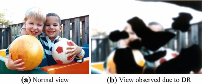
A qualitative comparison of normal vision and vision affected by Diabetic Retinopathy (DR) [30]

Researchers have proposed several methods for DR classification. Amin et al. [12] proposed a technique for exudates detection in fundus images. Jain et al.’s [11] approach using pretrained networks resulted in an accuracy of $80.40\%$. Pratt et al. [20] used the CNN method to classify DR stages, yielding a specificity, accuracy, and sensitivity of $95\%$, $75\%$, and $30\%$, respectively. Suriyal et al. [26] proposed a mobile application for real-time detection of DR with an accuracy of $73.3\%$. Masood et al. [16] discussed a transfer learning model supported Inception-V3 for DR detection on the EyePACS database with $48.2\%$ accuracy. Harun et al. [8] discussed a Multilayered perceptron trained with Bayesian regularization that provides a much better classification performance than the use of Levenberg–Marquardt with a training and testing accuracy of $72.11\%$, $67.47\%$, respectively. Wang, X. et al. [29] used pretrained models, AlexNet, VGG16, and Inception-v3, to classify DR. The average cross-validation accuracy of AlexNet, VGG16, and Inception-V3 are $37.43\%$, $50.03\%$, and $63.23\%$, respectively. A new pixel-wise score propagation model was proposed in [28] for the interpretable model for DR classification. Shankar et al. [22] have proposed a Synergic Deep Learning (SDL) model for DR image classification. In all such methods, the primary focus was to apply an off-the-shelf solution without getting into the network’s core, resulting in lower accuracy.

Recently, capsule network (CapsNet) got a lot of attention in medical technology as an alternative to CNN. Mobiny et al. [17] applied CapsNet in lung cancer screening and observed superior results than CNN when the training set is small. Afshar et al. [2] proposed COVID-CAPS, for COVID-19 detection using X-ray images with an accuracy of $95.7\%$, a sensitivity of $90\%$, specificity of $95.8\%$, and Area Under the Curve (AUC) of 0.97. Zhu et al. [33] introduce a method consisting of CNN and original capsule networks as a 1D deep capsule network and 3D deep capsule network for hyperspectral image classification. However, there has been no attempt to explore the possibility of CapsNet in DR classification.

This paper proposes DRISTI (Diabetic Retinopathy classIfication by analySing reTinal Images), a deep learning model for DR classification. The primary contributions of this paper are: (i) designing a hybrid deep learning model that combined VGG16 and the capsule network for the classification of retinal images into five classes (one non-DR and four DR classes), (ii) extensive experimental studies on six publicly available datasets and comparing the results with seven different state-of-the-art models to achieve the best performance, (iii) achieving almost $5\%$ gain over the best performing technique proposed in the literature.

The remaining of the paper is organized as follows. Details of the proposed methodology are given in Sect. 2. Section 3 gives a thorough explanation of the experimental study conducted in this work. In Sect. 4, the concluding remarks and future plans are highlighted.

Proposed methodology

Convolution neural networks (CNNs) have some limitations, and studies in the literature established that capsule networks could overcome some of these limitations [13]. After a thorough review of the papers on capsule networks, we concluded that pure convolution networks are not natively spatially invariant [13]. With pooling layers, convolution neural networks can learn the separating features of objects. However, they do not reflect the location of the item. These spatial features can seldom help determine the object’s class and hence affect the classification. The introduction of capsule networks fixes this approach and can model an object’s spatial or viewpoint variability in an image.

In the capsule network, neurons can encode the spatial information and the probability of an object being present [13]. This property of capsule networks makes it very encouraging in the case of medical image analysis. It is one of the motivations behind applying capsule networks to DR fundus images. Given the amount of data available in the publicly available datasets, we have adapted a transfer learning approach. We followed VGG16, Resnet50, Inceptionv3, and Xception architectures for the pretrained model because of their established effectiveness and ease of implementation. ImageNet, as a lot of transfer learning literature shows, is the best way to go in this case.

Network architecture

Figure 2 depicts the network structure of DRISTI, where a few intermediate layers are not shown for the sake of clarity. A literature review reveals that increasing the number of convolution layers allows the network to learn more buried features. Motivated by the fact that the deep neural network layers gradually know from simple to complex components from the samples, we decided to go for VGG16 and then increase the depth by using residual networks. Surprisingly, as shown in Sect. 3, our VGG16 model performs better than all other systems for both the two-class and five-class models. We have adapted the VGG16, Resnet50, and Xception networks in our framework. These networks are all pretrained on the ImageNet dataset.

Fig. 2.

A schematic illustration of the architecture of our proposed model DRISTI

CapsNets are capable of outperforming CNNs [21]. Table 1 shows the model parameters of DRISTI. We have replaced the top layers of the base model with our layer, which improved the results. In every capsule layer, a capsule yields a local grid of vectors to the type of capsule in the next layer. Then, the different transformation matrices for each grid member and each capsule type are used to obtain an equal number of classes. We have combined a convolution layer with an output depth of 256 and a kernel size of $7\times 7$ with a stride size of 1. We have passed the parameters 2, 16, and 4 to the two-class model capsule, while 5, 16, and 4 for the five-class model. The order of these parameters is the number of capsules, the capsules’ dimension, and routing. The remaining parameters passed to the capsule are set to the default value. Finally, we have used the margin loss with a batch size of 32, keeping the number of epochs set to 500.

Table 1.

Details of the network architecture of DRISTI

Layer (type)	Output Shape	Param#
Input1 (InputLayer)	(0, 224, 224, 3)	0
Conv1 (Conv2D)	(0, 224, 224, 64)	1792
Conv2 (Conv2D)	(0, 224, 224, 64)	36928
MaxPool2D	(0, 112, 112, 64)	0
Conv1 (Conv2D)	(0, 112, 112, 128)	73856
Conv2 (Conv2D)	(0, 112, 112, 128)	147584
MaxPool2D	(0, 56, 56, 128)	0
Conv1 (Conv2D)	(0, 56, 56, 256)	295168
Conv2 (Conv2D)	(0, 56, 56, 256)	590080
Conv3 (Conv2D)	(0, 56, 56, 256)	590080
MaxPool2D	(0, 28, 28, 256)	0
Conv1 (Conv2D)	(0, 28, 28, 512)	1180160
Conv2 (Conv2D)	(0, 28, 28, 512)	2359808
Conv3 (Conv2D)	(0, 28, 28, 512)	2359808
MaxPool2D	(0, 14, 14, 512)	0
Conv1 (Conv2D)	(0, 14, 14, 512)	2359808
Conv2 (Conv2D)	(0, 14, 14, 512)	2359808
Conv3 (Conv2D)	(0, 14, 14, 512)	2359808
MaxPool2D	(0, 7, 7, 512)	0
Conv1 (Conv2D)	(0, 1, 1, 256)	6422784
Reshape1 (Reshape)	(0, 1, 256)	0
Capsule1 (Capsule)	(0, 5, 16)	20480
Lambda1 (Lambda)	(0, 5)	0

Residual learning

Residual learning networks were proposed to ease the training of networks that are substantially deeper than those used previously [9]. The rationale of such a choice is their excellent performance on the ImageNet test set with an error of $3.57\%$. The number of filters is less compared to VGG16. The formal building blocks for residual networks are:

$$\begin{array}{c}\hfill y=\mathcal{F}(x,\{W_i\})+x.\end{array}$$ 1

Here, x, y are the input and output vectors. We need to learn the residual map represented by the function $\mathcal{F}$. These residual links speed up the convergence rate and avoid the problem of vanishing gradient.

Inception and Xception

Inception nets extracts feature by computing $1\times 1$, $3\times 3$, and $5\times 5$ convolutions within a network module. The correlation between channels is mapped differently from the spatial correlation [27] by decoupling the mapping of cross-channel correlation and spatial correlations in the feature maps of CNNs. The idea of the Xception network is based on depth-wise separable convolution layers [4]. The advantage of this architecture is that it is straightforward to define and highly customizable.

VGG16 model

The VGG16 model has an input size of $224\times 224$ during training, where an image is preprocessed by subtracting the mean RGB value for each pixel [24]. When the images pass through various network layers, filters with a small receptive field of size $3\times 3$ are used, with a stride of 1 pixel. The spatial padding is 1 pixel for $3\times 3$ convolution layers to preserve the spatial resolution. The spatial pooling is carried out by five max-pooling layers, which follow some (but not all) of the convolution layers. The max-pooling operation is performed with a stride of 2 on a $2\times 2$ pixel window. Three fully connected layers follow a stack of fully connected layers. The $1^{\mathit{st}}$ two fully connected layers have 4096 channels each, and the $3^{\mathit{rd}}$ one contains 1000 channels.

Loss function

The loss $(l_j)$ is calculated as [21]:

$$\begin{array}{c}\hfill l_j=A+\lambda B.\end{array}$$ 2

The first part (i.e., A) is calculated for the correct DR category, while the second part (i.e., B) is calculated for the incorrect DR category. The $\lambda$ coefficient, with a value of 0.5, is introduced in this context for numerical stability during the training process. The individual cost components are defined as:

$$\begin{array}{cc}& A=T_{j}max{(0,a-||s_j||)}^2\hfill \end{array}$$ 3

$$\begin{array}{cc}& B=(1-T_j)max{(0,||s_j||-b)}^2.\hfill \end{array}$$ 4

The terms $a$ and $b$ are hyperparameters and are set to 0.9 and 0.1, respectively. Whenever the DR class j is present, the term $T_j$ is 1, while for all other classes, which are absent for them, the value of $T_j$ is 0. We have calculated the total loss over the sum of the losses of every output capsule. In cases where $T_j$ will be 1 the first part of Eq. 2 will remain active. The value of a is set as 0.9, which means that when the l2 norm of $s_j$ is greater than 0.9, it is a 0 loss. Otherwise, it will be a nonzero loss. Therefore, if the probability of predicting the correct label is greater than 0.9, it is 0 loss. The second case will return a 0 loss if the correct label is not matched, and the probability of predicting an incorrect label is less than 0.1. In this case, $T_j$ is 0.

The loss of the decoder part is squared error and contributes less when compared to the capsules. We have done this to fix the networks and focus on the classification of the image. The final output $v_j$ for class j is computed as follows [21]:

$$\begin{array}{c}\hfill v_j=\frac{||s_j{||}^2}{1+||s_j{||}^2}\frac{s_j}{||s_j||}\end{array}$$ 5

where the prediction vector ${\widehat{u}}_{j|i}={\mathbf{W}}_{\mathit{ij}}{\mathbf{u}}_i$ and $v_j$ is the vector output of capsule j and $s_j$ is its total input.

$$\begin{array}{c}\hfill s_j=\sum _i{c}_{\mathit{ij}}{\widehat{u}}_{j|i}.\end{array}$$ 6

Transfer learning for DR classification

Given a source domain $\mathcal{S}$ and learning task $\mathcal{T}$, a target domain $\mathcal{D}$ and learning task $\mathcal{T}$, transfer learning aims to help improve the learning of the target predictive function $f_{\mathcal{T}}()$ in $\mathcal{D}$ using the knowledge in $\mathcal{S}$ and $\mathcal{T}$. Here, the notable concept is $\mathcal{S}\ne \mathcal{D}$ , or $\mathcal{T}\ne \mathcal{T}$. In the context of recognition task for cross-dataset testing, the goal of transfer learning is to learn a robust classifier $\mathcal{F}(.)$ from a dataset (i.e., target dataset $D_{\mathcal{T}}$) by effectively utilizing the knowledge offered through other datasets (i.e., source datasets $D_{\mathcal{S}}$). In DRISTI, a pretrained model on ImageNet is used. Hence, $\mathcal{S}$ is the domain of natural images, and $\mathcal{T}$ is various tasks in ImageNet. In our case, neither the source domain’s samples are related to DR detection nor the task. The target domain ($\mathcal{D}$) in our case is the domain of retinal images, and the learning task ($\mathcal{T}$) is DR classification. In DRISTI, we repurpose the learned features by learning the mapping function $\mathcal{F}(.)$ from the $\mathcal{S}$ into $\mathcal{D}$.

Experiment and results

The model is trained on Nvidia DGX II, using Python 3.7. We have used API Keras version 2.2.4, Tensorflow-GPU version 1.14, Seaborn 0.9.0, Scikit learn 0.21.3 that were used to implement the proposed framework.

Dataset

DRISTI is evaluated by performing experiments on IDRiD [19], DIARETDB1 [14], DIARETDB0 [15], STARE [10], DRIVE [18], and MESSIDOR-2 [1, 5] datasets. Figure 3 depicts a few samples from these datasets. Table 2 summarizes the details of the datasets. The target of any deep neural network approach is to learn the optimal set of parameters during training. With the increasing number of learnable parameters, the model demands a large number of training samples. The number of examples available in the publicly available dataset used for DR detection is few compared to standard image datasets used to train any deep neural network model. We account for these situations by introducing our neural network with an augmented dataset (see Sect. 3.8).

Fig. 3.

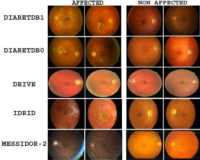
Sample images showing affected and non-affected retina images from various datasets

Table 2.

Details of the datasets used in experiments

Dataset	# Samples	Classes
IDRiD	331	2
DIARETDB1	89	2
DIARETDB0	130	2
STARE	161	2
DRIVE	40	2
MESSIDOR-2	900	5

Results

DRISTI’s performance is compared with other state-of-the-art models (see Table 3), where the boldface values indicate the best performance. The five-class model has performed better than even some two-class state-of-the-art models. Moreover, our two-class model has outperformed every other model on the list. For five classes, the highest training accuracy achieved is $99.60\%$, the highest validation accuracy achieved is $82.06\%$, and the test accuracy obtained is $75.81\%$. For the two classes, the highest training accuracy achieved is $99.74\%$, the highest validation accuracy we have achieved is $96.24\%$, and the test accuracy obtained is $95.50\%$. The confusion matrices for the two-class and the five-class setting are shown in Fig. 4a and b, respectively. The accuracy and loss graphs for the two-class and the five-class model are shown in Fig. 5. These plots indicate the training and validation process of DRISTI.

Table 3.

Comparison of classification accuracy of several state-of-the-art methods with DRISTI

Method	Approach	Accuracy
[32]	CNN	44.22%
[25]	CNN	56%
[25]	CNN (two-class)	71%
[23]	CAD system (two-class)	93.75%
[29]	Pretrained model	63.23%
[3]	CNN	74%.
[7]	VGG16 CNN	75.83%
Ours	VGG16+Capsule (five-class)	82.06%
	VGG16+Capsule (two-class)	96.24%

Fig. 4.

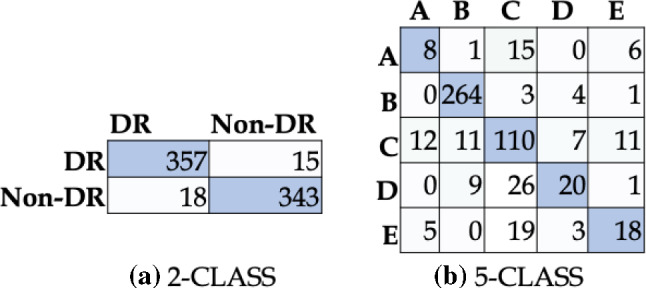
Confusion matrix for a two-class and b five-class classification performance of DRISTI. In (b), the five classes are A: Severe, B: No-DR, C: Moderate, D: Mild, E: Proliferate-DR

Fig. 5.

Graphs of accuracy and loss for two-class and five-class problems during training and validation

Ablation study

In models like DRISTI having intermediate processing stages, it is important to study the influence of intermediate stages. We have done an ablation study and compared our model by changing the base model with different architectures. Such a comparison based on primary metrics is undertaken. Table 4 shows the ablation study results on the datasets. The base capsule model is also used for comparison, and the results are presented in the same table. The bold face values show the best performance across all variants. We can see that the VGG16 performs the best for two classes as the five-class models when we compare it by the validation accuracy. The Resnet50 model for two classes closely follows it, but the Xception network outperforms the Resnet50 for five classes. To summarize the research findings, we have presented Tables 5 and 6 to show the precision, recall, and F1-score of the predicted result for the five classes and the two-class model, respectively, with the base model as VGG16.

Table 4.

Experimental results in terms of classification accuracy on ablation study

Approach	Max Train Acc.	Max Valid Acc.
VGG16 + Capsule (two-class)	99.74%	96.24%
VGG16 + Capsule (five-class)	99.60%	82.06%
Resnet50 + Capsule (two-class)	98.89%	96.07%
Resnet50 + Capsule (five-class)	96.73%	76.80%
Inception3 + Capsule (two-class)	99.91%	95.05%
Inception3 + Capsule (five-class)	99.36%	76.41%
Xception + Capsule (two-class)	100%	95.22%
Xception + Capsule (five-class)	99.46%	79.53%.
Capsule Network (two-class)	95.13%	93.68%
Capsule Network (five-class)	81.79%	74.07%

Table 5.

Classification result of the five-class problem

Level	Precision	Recall	F1-score	Support
Severe	0.32	0.27	0.29	30
Normal	0.93	0.97	0.95	272
Moderate	0.64	0.73	0.68	151
Mild	0.59	0.36	0.44	56
Proliferative	0.49	0.40	0.44	45

Table 6.

Classification result of the two-class problem

Level	Precision	Recall	F1-score	Support
DR	0.95	0.96	0.96	372
Normal	0.96	0.95	0.95	361

Performance on unseen samples

Learning paradigms assume that the training and test data belong to the same distribution. However, when we deal with the real-world scenario, we often come across test data with different distributions than the training data. To investigate how DRISTI performs on unseen data, we have conducted experiments on unseen samples. Figure 6 depicts a few such unseen examples and DRISTI’s performance on them. The label at the top of each instance represents the prediction and the actual values. The samples shown here are a portion of the examples that are used for testing. Here, we can see that some of the categories are predicted incorrectly. For example, the first sample of the fourth row is predicted as No-DR. However, it belongs to the DR class.

Fig. 6.

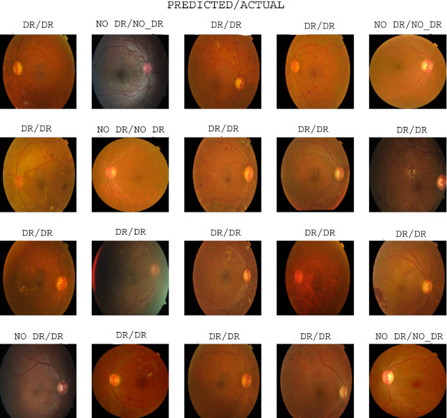
Qualitative results of DRISTI showing the predicted vs. actual class labels for the two-class problem

Cross-dataset testing

We have tested our highest performing VGG16 with the CapsNet model on completely unknown samples. Out of the datasets mentioned, we had taken the dataset MESSIDOR-2 for five-class classification as it has appropriately labeled five-class images. We have used our top-performing five-class model to test on MESSIDOR-2. The rest of the datasets have been tested in two classes. The testing accuracy of our VGG16 model is shown in Fig. 7a. We can see that the accuracy with the IDRiD dataset is highest by a margin of $2.39\%$ when compared to the second highest DRIVE dataset for two classes. A possible reason for such observation could be the Indian context of APTOS (training) and IDRiD (testing) datasets.

Fig. 7.

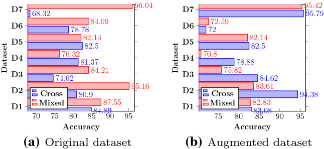
Quantification of cross-dataset and mixed dataset performance of DRISTI on D1:IDRiD, D2:DIARETDB1, D3:DIARETDB0, D4:STARE, D5:DRIVE, D6:MESSIDOR-2, D7:APTOS datasets

Experiments on mixed dataset

A single dataset contains a limited number of signature samples and fails to capture the input space’s entire gamut. To see the effect on DRISTI’s performance while introducing samples from other datasets, we have randomly taken $30\%$ of each dataset and combined them to create a mixed dataset. The training and testing have been performed by splitting the dataset into a proportion of $65\%$ training and $35\%$ testing. The two-class classification results of this version of DRISTI are shown in Fig. 7a. The APTOS dataset is the best performer due to the more number of images received during training. It even crosses the validation accuracy of the mixed dataset on which the model was trained. The mixed dataset performs better than or equal to every other test done on the cross-dataset except on the STARE dataset. The rationale for this is the highly unbalanced nature of the dataset when converted to a two-class. This is also a possible reason for such improved performance on the images trained on APTOS than when trained on a mixed dataset. The five-class classification has not been shown as most of the datasets that we have used and available in the literature are two-class, so it was impossible to create a proper five-class mixed dataset for performing training.

Impact of training size

The exploitation of high-order complex data raises new research challenges due to the high dimensionality and the limited number of ground truth samples. The number of training samples is a critical factor that determines a model’s classification accuracy. Figure 8 depicts the effect of change of training samples on the performance of DRISTI. The horizontal and vertical axes represent the number of image samples and the percentage accuracy, respectively. In the single image set, we see that neither the training accuracy nor the testing accuracy improves drastically but shows signs of progress. For the mixed dataset, we see a peak presented in Fig. 8b. This is because a 65 percent mark shows the best result, i.e., we get the best testing accuracy when the ratio of training to testing is 65:35. Hence, for DRISTI, we have chosen $65\%$ of samples for training.

Fig. 8.

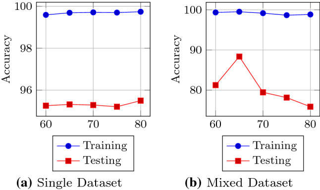
An illustration of the effect of number of training samples on DRISTI’s performance

A study on an augmented dataset

We have augmented the APTOS-19 dataset by changing the rotation range, width, and height shift range. The images have been horizontally flipped with a low shear and zoom range of 0.2 to keep the distinguishing features. We have done this to ensure that the model holds valid for a bigger dataset, thus being more general. Figure 7b depicts the cross-dataset’s testing results and mixed dataset scenarios. We use 29, 101 augmented images for five-class, and the highest training and validation accuracy obtained is $99.91\%$ and $75.50\%$, respectively. We tested the five-class model on 546 images and got a testing accuracy of $74.73\%$. We have also extended our previous two-class cross-dataset, and mixed dataset models to the two-class augmented dataset. We use 21, 024 images from augmented APTOS for training on two classes. The number of images is lesser than five classes to balance the two types. The highest training and validation on the two-class augmented APTOS dataset is $99.96\%$ and $97.05\%$, respectively. For the mixed dataset, we have used 29, 009 for images. Additional 8000 images are augmented and collected from the different datasets mentioned in Fig. 7. Our curated dataset has $70\%$ of the expanded APTOS dataset and $30\%$ of the remaining un-augmented datasets. The process is similar to how we created a mixed dataset in the previous section except for the augmentation. The highest training and validation accuracies are $99.92\%$ and $91.43\%$, respectively. We see an opposite scenario when compared to training on an un-augmented APTOS. The mixed augmented dataset has not performed very well when compared to the cross-dataset. Augmenting the dataset changes the difference between images and decreases the separability between them. That is why creating a mixed dataset on such extended results further confuses the model, lowering the effects.

Statistical significance test

We followed the two-proportion Z-test to justify whether the differences between different algorithms (and their variants) are essential in the statistical sense. Here, the proportion means that the average percentage accuracy of DRISTI across the dataset. The null hypothesis for the test is that the proportions are the same, while the alternative hypothesis is that the proportions are not the same. In our experiments, we have considered an alpha level of $5\%$. The Z-score obtained in our case is 7.68. Comparing the calculated Z-score with the table Z-score (1.96) shows Z-score is larger. Hence, we rejected the null hypothesis and claim that DRISTI has significantly better performance over others.

Conclusion

This paper presents DRISTI, a combination of VGG16 and capsule networks, to classify DR from retinal images. DRISTI performs with an overall validation accuracy of $82.06\%$ and testing accuracy of $75.81\%$ for five-class and $96.24\%$ validation accuracy and $95.50\%$ testing accuracy for two-class classification. The experiment also shows that our classification system can assist the oculist in diagnosing DR accurately with more speed and could potentially boost DR patients’ screening rate. The dataset that we have used for our experiment was unbalanced for the class distribution. If we use an improved dataset, then the results can be improved. We have also done testing on a cross-dataset to show that our model is robust for unknown data.

References

- 1.Abràmoff MD, Folk JC, Han DP, Walker JD, Williams DF, Russell SR, Massin P, Cochener B, Gain P, Tang L, Lamard M, Moga DC, Quellec G, Niemeijer M. Automated analysis of retinal images for detection of referable diabetic retinopathy. JAMA Ophthalmol. 2013;131(3):351–357. doi: 10.1001/jamaophthalmol.2013.1743. [DOI] [PubMed] [Google Scholar]
- 2.Afshar, P., Heidarian, S., Naderkhani, F., Oikonomou, A., Plataniotis, K.N., Mohammadi, A.: Covid-caps: a capsule network-based framework for identification of covid-19 cases from x-ray images (2020) [DOI] [PMC free article] [PubMed]
- 3.Arora, M., Pandey, M.: Deep neural network for diabetic retinopathy detection. In: COMITCon (2019)
- 4.Chollet, F.: Xception: deep learning with depthwise separable convolutions (2016)
- 5.Decencière E, Zhang X, Cazuguel G, Lay B, Cochener B, Trone C, Gain P, Ordonez R, Massin P, Erginay A, Charton B, Klein JC. Feedback on a publicly distributed image database: the messidor database. Image Anal. Stereol. 2014;33(3):1005. doi: 10.5566/ias.1155. [DOI] [Google Scholar]
- 6.Duh E, Sun J, Stitt A. Diabetic retinopathy: current understanding, mechanisms, and treatment strategies. JCI Insight. 2017;2(14):1000. doi: 10.1172/jci.insight.93751. [DOI] [PMC free article] [PubMed] [Google Scholar]
- 7.G, N., C, S.S., Chandra G R, H., M, I.: Deep learning framework for diabetic retinopathy diagnosis. In: 2019 3rd International Conference on Computing Methodologies and Communication (ICCMC) (2019)
- 8.Harun, N.H., Yusof, Y., Hassan, F., Embong, Z.: Classification of fundus images for diabetic retinopathy using artificial neural network. In: IEEE Jordan International Joint Conference on Electrical Engineering and Information Technology (JEEIT) (2019)
- 9.He, K., Zhang, X., Ren, S., Sun, J.: Deep residual learning for image recognition (2015)
- 10.Hoover, A.: Structured analysis of the retina stare (2015)
- 11.Jain, A., Jalui, A., Jasani, J., Lahoti, Y., Karani, R.: Deep learning for detection and severity classification of diabetic retinopathy. In: ICIICT (2019)
- 12.Javeria A, Muhammad SYM, Hussam A, Steven LF. A method for the detection and classification of diabetic retinopathy using structural predictors of bright lesions. J. Comput. Sci. 2017;19:153–164. doi: 10.1016/j.jocs.2017.01.002. [DOI] [Google Scholar]
- 13.Jiménez-Sánchez, A., Albarqouni, S., Mateus, D.: Capsule networks against medical imaging data challenges. Lecture Notes in Computer Science, pp. 150–160 (2018)
- 14.Kauppi, T., Kalesnykiene, V., Kämäräinen, J.K., Lensu, L., Sorri, I., Raninen, A., Voutilainen, R., Uusitalo, H., Kälviäinen, H., Pietilä, J.: The diaretdb1 diabetic retinopathy database and evaluation protocol. In: BMVC (2007)
- 15.Kauppi, T., Kalesnykiene, V., Kämäräinen, J.K., Lensu, L., Sorri, I., Uusitalo, H., Kälviäinen, H., Pietilä, J.: Diaretdb 0: evaluation database and methodology for diabetic retinopathy algorithms (2007)
- 16.Masood, S., Luthra, T., Sundriyal, H., Ahmed, M.: Identification of diabetic retinopathy in eye images using transfer learning. In: ICCCA (2017)
- 17.Mobiny A, Van Nguyen H. Fast capsnet for lung cancer screening. In: Frangi AF, Schnabel JA, Davatzikos C, Alberola-López C, Fichtinger G, editors. Medical Image Computing and Computer Assisted Intervention - MICCAI 2018. Cham: Springer International Publishing; 2018. pp. 741–749. [Google Scholar]
- 18.Niemeijer, M., Staal, J., Ginneken, B., Loog, M., Abramoff, M.: Drive: digital retinal images for vessel extraction. Methods for Evaluating Segmentation and Indexing Techniques Dedicated to Retinal Ophthalmology (2004)
- 19.Prasanna, P., Samiksha, P., Ravi, K., Manesh, K., Girish, D., Vivek, S., Meriaudeau, F.: Indian diabetic retinopathy image dataset (idrid) (2018) 10.21227/H25W98
- 20.Pratt H, Coenen F, Broadbent D, Harding SP, Zheng Y. Convolutional neural networks for diabetic retinopathy. Procedia Comput. Sci. 2016;90:200–205. doi: 10.1016/j.procs.2016.07.014. [DOI] [Google Scholar]
- 21.Sabour, S., Frosst, N., Hinton, G.E.: Dynamic routing between capsules. In: CoRR (2017)
- 22.Shankar, K., Rahaman Wahab Sait, A., Gupta, D., Lakshmanaprabu, S.K., Khanna, A., Pandey, H.M.: Automated detection and classification of fundus diabetic retinopathy images using synergic deep learning model. PRL 133, 210–216 (2020)
- 23.Shojaeipour, A., Nordin, M.J., Hadavi, N.: Using image processing methods for diagnosis diabetic retinopathy. In: ROMA (2014)
- 24.Simonyan, K., Zisserman, A.: Very deep convolutional networks for large-scale image recognition (2014)
- 25.Singh, T.M., Bharali, P., Bhuyan, C.: Automated detection of diabetic retinopathy. In: ICACCP (2019)
- 26.Suriyal, S., Druzgalski, C., Gautam, K.: Mobile assisted diabetic retinopathy detection using deep neural network. In: GMEPE/PAHCE (2018)
- 27.Szegedy, C., Liu, W., Jia, Y., Sermanet, P., Reed, S., Anguelov, D., Erhan, D., Vanhoucke, V., Rabinovich, A.: Going deeper with convolutions (2014)
- 28.de la Torre J, Valls A, Puig D. A deep learning interpretable classifier for diabetic retinopathy disease grading. Neurocomputing. 2019;3:57. [Google Scholar]
- 29.Wang, X., Lu, Y., Wang, Y., Chen, W.: Diabetic retinopathy stage classification using convolutional neural networks. In: 2018 IEEE International Conference on Information Reuse and Integration (IRI) (2018)
- 30.Wikipedia contributors: diabetic retinopathy—Wikipedia, the free encyclopedia (2020) https://en.wikipedia.org/wiki/Diabetic_retinopathy
- 31.Wu L, Fernandez-Loaiza P, Sauma J, Hernandez-Bogantes E, Masis M. Classification of diabetic retinopathy and diabetic macular edema. World J. Diabetes. 2013;4:290–294. doi: 10.4239/wjd.v4.i6.290. [DOI] [PMC free article] [PubMed] [Google Scholar]
- 32.Zehra, F., Faran, M., Anjum, A., Islam, S.: Dr-net: Cnn model to automate diabetic retinopathy stage diagnosis. In: UPCON (2019)
- 33.Zhu K, Chen Y, Ghamisi P, Jia X, Benediktsson JA. Deep convolutional capsule network for hyperspectral image spectral and spectral-spatial classification. Remote Sens. 2019;11(3):223. doi: 10.3390/rs11030223. [DOI] [Google Scholar]