Computing Absolute Free Energy with Deep Generative Models

Abstract

Fast and accurate evaluation of free energy has broad applications from drug design to material engineering. Computing the absolute free energy is of particular interest since it allows the assessment of the relative stability between states without intermediates. Here we introduce a general framework for calculating the absolute free energy of a state. A key step of the calculation is the definition of a reference state with tractable deep generative models using locally sampled configurations. The absolute free energy of this reference state is zero by design. The free energy for the state of interest can then be determined as the difference from the reference. We applied this approach to both discrete and continuous systems and demonstrated its effectiveness. It was found that the Bennett acceptance ratio method provides more accurate and efficient free energy estimations than approximate expressions based on work. We anticipate the method presented here to be a valuable strategy for computing free energy differences.

Graphical Abstract

INTRODUCTION

Free energy is of central importance in both statistical physics and computational chemistry. It has important applications in rational drug design¹ and material property prediction.² Therefore, methodology development for efficient free energy calculations has attracted great research interest.^3–14 Many existing algorithms have focused on estimating free energy differences between states and originate from the free energy perturbation (FEP) identity¹⁵

$${\mathbb{E}}_A[e^{-\beta \Delta U}]=e^{-\beta \Delta F}.$$ (1)

Here, ΔF = F_B − F_A is the free energy difference between two equilibrium states A and B at temperature T and β = 1/k_BT. U_A(x) and U_B(x) are the potential energies for a configuration x in states A and B, respectively, and ΔU (x) = U_B(x)−U_A(x). ${\mathbb{E}}_A$ represents the expectation with respect to the Boltzmann distribution of x in state A,

$$p_A(x)=\frac{e^{-\beta U_A(x)}}{Z_A},$$ (2)

where the normalization constant $Z_A=\int e^{-\beta U_A(x)}dx$. Computing ΔF with the FEP identity (Eq. 1) only uses samples from state A. It is more efficient to use samples from both states to compute ΔF by solving the Bennett acceptance ratio (BAR) equation ¹⁶

$$\begin{gathered} \sum _{k=1}^{N_A}f(\beta [\Delta U(x_k^A)-M-\Delta F]) \\ =\sum _{k=1}^{N_B}f(-\beta [\Delta U(x_k^B)-M-\Delta F])), \end{gathered}$$ (3)

where f(t) = 1/(1 + e^t) and M = ln(N_B/N_A). Here, $\left\{x_k^A,k=1,\dots ,N_A\right\}$ and $\left\{x_k^B,k=1,\dots ,N_B\right\}$ are samples from the two states. Both the FEP and the BAR method converge poorly when the overlap in the configuration space between state A and B is small. In that case, multiple intermediate states along a path with incremental changes in the configuration space can be introduced to bridge the two states.³ However, sampling from multiple intermediate states greatly increases the computational cost. It is, therefore, useful to develop techniques that can alleviate the convergence issue without the use of intermediate states.^12,13

The requirement on a significant overlap between the two states’ configuration space can be circumvented if we compute their free energy difference from the absolute free energy as ΔF = F_B − F_A. The absolute free energy of a state A/B can be obtained from its difference from a reference state A±/B± as F_A/B = F_A±/B± − ΔF_A/B→A±/B±. For this strategy to be efficient, however, the reference states must bear significant overlap in configuration space with the states of interest. Their absolute free energy should be available with minimal computational effort. For most systems, designing reference states that satisfy these constraints can be challenging and requires expertise and physical intuition.^17–23 In this work, we demonstrate that reference states can be constructed with tractable generative models for efficient computation of the absolute free energy. ^24,25

COMPUTATIONAL METHODS

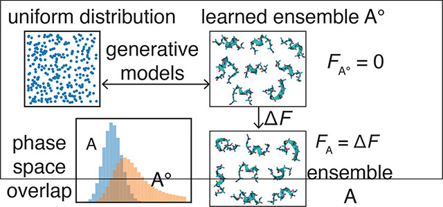
The workflow for calculating the absolute free energy is as follows. State A is used as an example for the discussion, but the same procedure applies to state B. We first draw samples, $\left\{x_k^A,k=1,\dots ,N_A\right\}$, from the Boltzmann distribution p_A(x). We then learn a tractable generative model, q_θ(x), that maximizes the likelihood of observing these samples by fine-tuning the set of parameters θ. Here tractable generative models refer to probabilistic models that have the following two properties: (i) the normalized probability (or probability density), q_θ(x), can be directly evaluated for a given configuration x without the need of sampling or integration; (ii) independent configurations can be efficiently sampled from the probability distribution. The generative model defines a new equilibrium state A±, which serves as an excellent reference to state A. Because it is parameterized from samples of state A, most probable configurations from A± should resemble those from A by design, and the overlap between the two states is guaranteed as long as the generative model has enough flexibility for modeling p_A(x). In addition, since q_θ(x) is normalized, if we define the potential energy of state A± as U_A± (x) = −(1/β) ln q_θ(x), the partition function Z_A± of state A± is equal to 1, i.e., $Z_{A\circ }=\int q_{\theta }(x)\text{d}x=1$. The absolute free energy of the reference state A± is F_A± = −(1/β) ln Z_A± = 0. (Strictly speaking, the free energy should be defined as $F_{A\circ }=-(1/\beta )\ln \left(Z_{A^{°}}/\int 1\text{d}x\right)$ to normalize the unit in the partition function. This technical detail does not affect any of the conclusions on free energy differences and is not considered for simplicity.) With the reference state defined, the absolute free energy for state A can be determined by solving a similar BAR equation as Eq. 3. Our use of tractable generative models ensures that sample configurations can be easily produced for the reference state to be combined with those from state A for solving the BAR equation. ²⁶

We note that a closely related algorithm for computing the absolute free energy has been introduced in variational methods.^27,28 In these prior studies, q_θ(x) was optimized by minimizing the Kullback-Leibler (KL) divergence²⁹ from q_θ(x) to p_A(x)

$$\begin{gathered} D_{\text{KL}}\left(q_{\theta }\Vert p_A\right)=\int q_{\theta }(x)\ln \frac{q_{\theta }(x)}{p_A(x)}\text{d}x \\ =\beta \left(\langle W_{A\circ \to A}\rangle -F_A\right), \end{gathered}$$ (4)

where $\langle W_{A\circ \to A}\rangle ={\mathbb{E}}_{A\circ }\left[U_A(x)-U_{A\circ }(x)\right]$. Because D_KL(q_θ‖p_A) is non-negative, ⟨W_A±→A⟩ is an upper bound of F_A. As D_KL(q_θ‖p_A) decreases along the optimization, ⟨W_A±→A⟩ is assumed to approach closer to the true free energy and was used for its estimation.

Our methodology is different from the variational methods^27,28,30 in two aspects. Firstly, instead of D_KL(q_θ‖p_A), we used

$$\begin{gathered} D_{\text{KL}}\left(p_A\Vert q_{\theta }\right)=\int p_A(x)\ln \frac{p_A(x)}{q_{\theta }(x)}\text{d}x \\ =\beta \left(\langle W_{A\to A\circ }\rangle +F_A\right) \end{gathered}$$ (5)

as the objective function for learning q_θ(x). $\langle W_{A\circ \to A}\rangle ={\mathbb{E}}_A\left[U_{A\circ }(x)-U_A(x)\right]$. We note that minimizing the KL divergence from p_A(x) to q_θ(x) is equivalent to learning the generative model by maximizing its likelihood on the training data. Moreover, because D_KL(p_A‖q_θ) is also non-negative, ⟨−W_A→A± ⟩ is a lower bound of F_A. Therefore, minimizing D_KL(p_A‖q_θ) is equivalent to maximizing the lower bound ⟨−W_A→A± ⟩. At the face value, it may seem that D_KL(q_θ‖p_A) is a better objective function than D_KL(p_A‖q_θ) for model training since its optimization only requires samples from q_θ(x). As aforementioned, sampling from q_θ(x) can be made computationally efficient by the use of tractable generative models. On the other hand, training by D_KL(p_A‖q_θ) requires samples from p_A(x), the collection of which often requires costly long timescale simulations with Monte Carlo (MC) or molecular dynamics (MD) techniques. The caveat is that optimization with D_KL(q_θ‖p_A) is more susceptible to traps from local minima due to its more complex dependence on q_θ.³¹ When p_A(x) is a high-dimensional distribution and the system exhibits multistability, optimizing D_KL(q_θ‖p_A) often leads to solutions that cover only one of the metastable states.^32,33 Noé and coworkers have recognized the above challenge,³² and they introduced the Boltzmann generator that uses a combination of both D_KL(q_θ‖p_A) and D_KL(p_A‖q_θ) for model training.

Another significant difference between our methodology and the variational methods^27,28,34 or the Boltzmann generator is the expression used to estimate F_A. In particular, ⟨W_A±→A⟩ is an upper bound of the free energy and only becomes exact when the probability distributions from generative models and the state of interest are identical. On the other hand, our use of the BAR equation (Eq. 3) relaxes this requirement, and F_A can be accurately determined even if the model training is not perfect and there are significant differences between the two distributions. In all but trivial examples, we anticipate that the learning process does not converge exactly to the true distribution p_A(x) due to its high dimensionality and complexity. The BAR estimation, which is asymptotically unbiased, ³⁵ will be crucial to ensure the accuracy of free energy calculations.

RESULTS

The advantage of the BAR estimation is evident when computing the absolute free energy of a two-dimensional system with the Müller potential.³⁷ When the reference state q_θ(x) was parameterized with a Gaussian distribution, which fails to capture the multistability inherent to the system, the two bounds based on work deviate significantly from the absolute free energy (Fig. 1). The free energy estimated using the BAR equation, on the other hand, is in excellent agreement with the exact value. The work-based bounds begin to approach the exact value when an optimized mixture model of two Gaussian distributions was used to parameterize the reference state. The BAR estimator again converges much faster than the bounds, highlighting its insensitivity to the quality of the reference state. More details about the model training and free energy computation for this simple test system are included in the Supporting Information. We note that an independent study reported similar advantages when using BAR to compute relative free energy with deep generative models. ¹³

Figure 1:

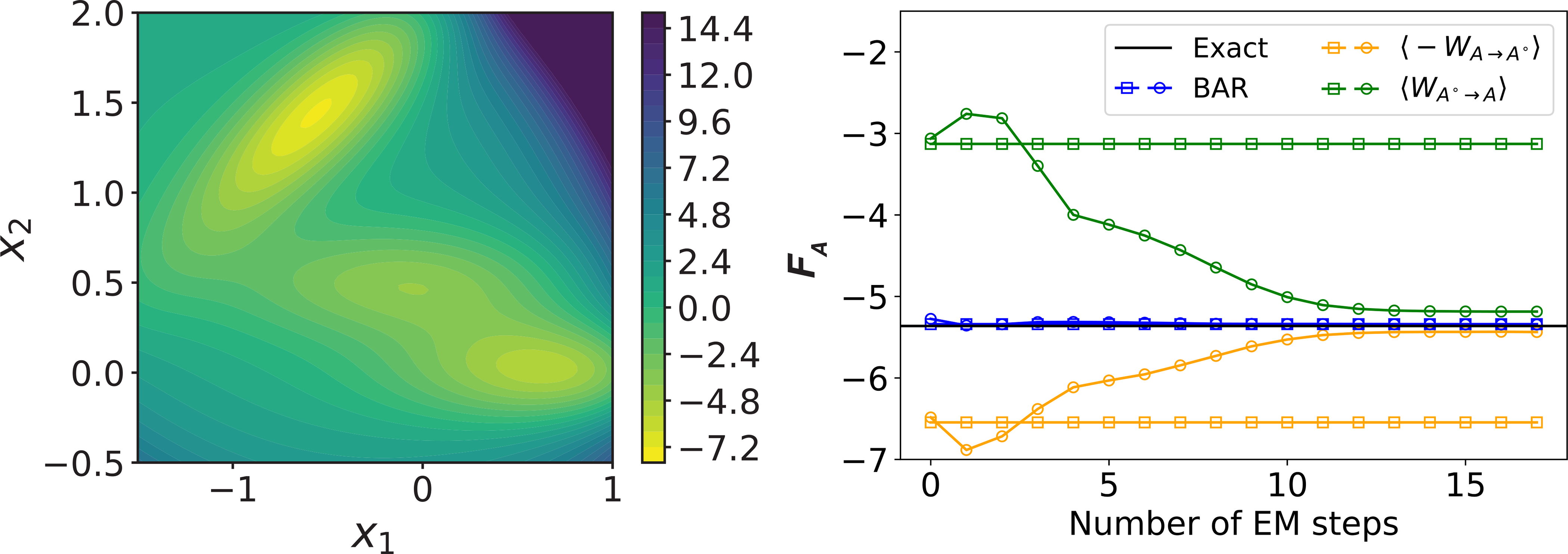
(Left) Contour plot of the Müller potential. Energy is shown in the units of k_BT. (Right) Absolute free energy computed using various estimators with reference states defined as a Gaussian distribution (squares) or a mixture model of two Gaussian distributions (circles). The x-axis corresponds to the number of steps for training the Gaussian mixture model with the expectation-maximization (EM) algorithm. ³⁶

Encouraged by the results from the above test system, we next computed the absolute free energy of a 20-spin classical Sherrington-Kerkpatrick (SK) model,³⁸ the value of which can be determined from complete enumeration as well. The discrete configurations of the SK model will be represented using s instead of x. Though we introduced the methodology with continuous variables, all the equations can be trivially extended to s by replacing the integrals with summations over the spin configurations. The potential energy of a configuration s = (s₁, s₂, ..., s_N ) is defined as

$$U_A(\mathbf{s})=\frac{1}{\sqrt{N}}\sum _{j>i}{J}_{ij}{s}_i{s}_j,$$ (6)

where s_i ∈ {−1, +1} and N = 20. J_ij were chosen randomly from the standard normal distribution. 5000 samples were drawn from the probability distribution $p(s)=e^{-\beta U_A(s)}/Z_A$ with β = 2.0. These samples were used to train the reference state A± by minimizing D_KL(p_A‖q_θ) (Eq. 5). The reference probability q_θ(s) was defined with a neural autoregressive density estimator (NADE)^24,39–42 as a product of conditional distributions

$$q_{\theta }(s)=\prod _{i=1}^N{q}_{\theta }\left(s_i\mid s_1,\dots ,s_{i-1}\right).$$ (7)

q_θ(s_i|s₁, ..., s_i−1) were parameterized using a feed-forward neural network with one hidden layer of 20 hidden units.The neural network’s connections are specifically designed such that it maintains the autoregressive property, i.e., q_θ(s_i|s₁, ..., s_i−1) only depends on s₁, ..., s_i (Fig. 2a). After training q_θ(s) for some numbers of steps, ^43,44 5000 configurations were independently drawn from q_θ(s). These configurations, together with the training inputs sampled from p_A(s), were used to determine the absolute free energy of the SK model. In Figs. 2b and 2c, we again compare results from the three estimators with the exact value.

Figure 2:

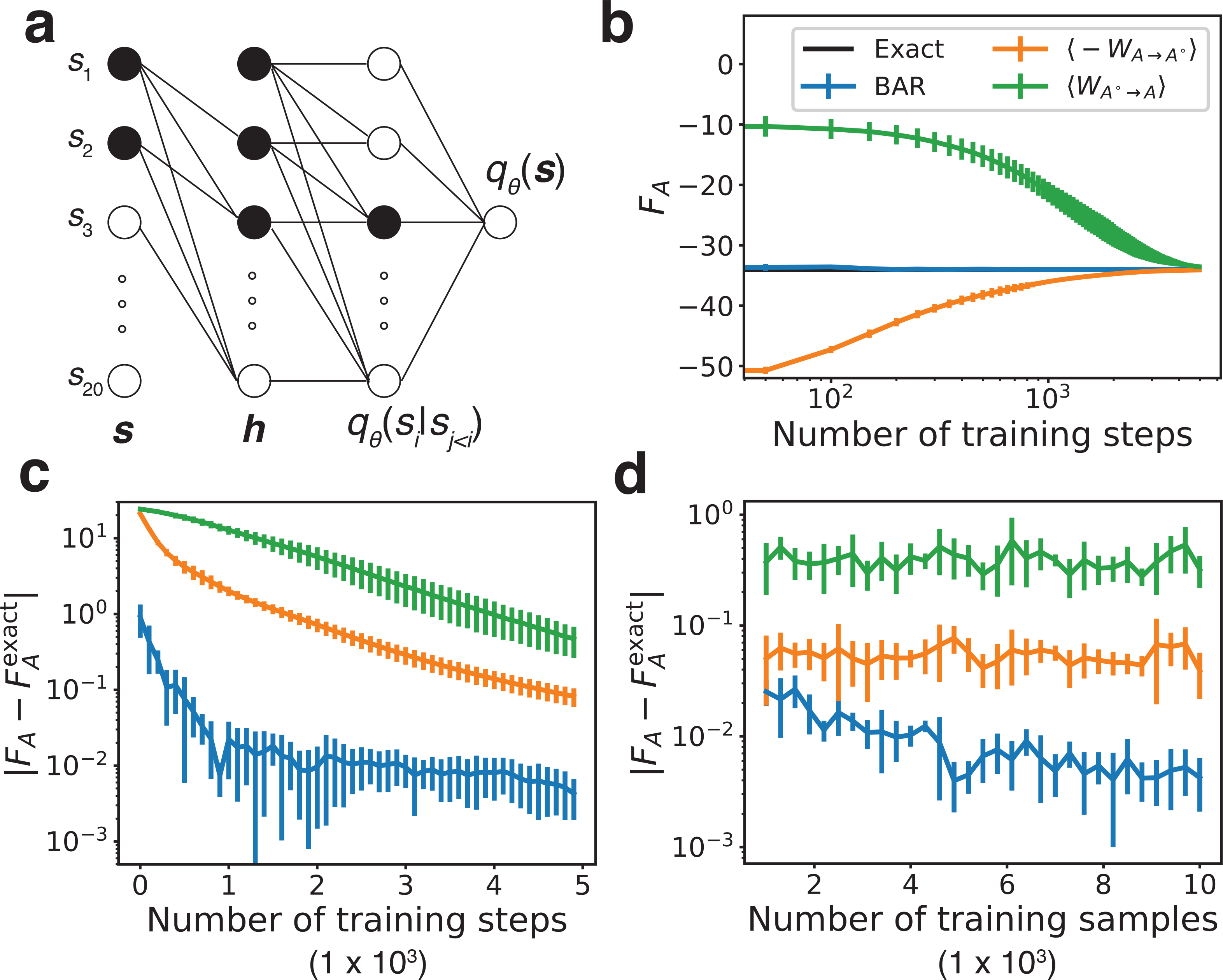
Performance of different free energy estimators on the SK model. Energy is shown in the units of k_BT. (a) A schematic representation of the neural autoregressive model used to parameterize q_θ. The black units illustrate the dependence of the conditional probability q(s₃|s₁, s₂). (b) The absolute free energy of the SK model calculated with three estimators as a function of training steps compared with the exact result obtained from a complete enumeration. (c, d) Errors of the estimated absolute free energy versus the number of training steps and the number of samples used for training q_θ. The coloring scheme is identical to that in part b. Error bars representing one standard deviation are estimated using five independent repeats.

Similar to the results observed for the Müller potential, at early stages of model parameterization with small training step numbers, the work-based estimations deviate significantly from the true value. This deviation is expected and is a direct result of the difference between the two probability distributions q_θ(s) and p_A(s). However, as the training proceeds, the agreement between the distributions improves and ⟨−W_A→A± ⟩ and ⟨W_A±→A⟩ gradually converge to the exact result after 5000 steps (Fig. 2b) because the autoregressive model is flexible enough to match the target distribution. On the other hand, the BAR estimator converges much faster to the exact value with a smaller error (Figs. 2b and 2c). In addition, varying the number of samples used for training q_θ(s) has different effects on the accuracy of converged results for the three approaches (Fig. 2d). For both ⟨−W_A→A± ⟩ and ⟨W_A±→A⟩, increasing the number of training samples from 10³ to 10⁴ does not significantly change the accuracy of their results. In contrast, using more training samples significantly reduces the error of the BAR estimator. This is because solutions of the BAR equation are asymptotically unbiased for estimating F_A, whereas ⟨−W_A→A± ⟩ and ⟨W_A±→A⟩ are not.³⁵

Finally, we applied the methodology to two molecular systems, the di-alanine and the deca-alanine in implicit solvent. These two systems present features commonly encountered in biomolecular simulations with continuous phase space over a rugged energy landscape. Their high dimensionality renders a complete enumeration of the configurational space to compute the absolute free energy for benchmarking impractical. Instead, we calculated the free energy difference between two metastable states using their absolute free energy to compare against the value determined from umbrella sampling and temperature replica exchange (TRE) simulations. For di-alanine, the two metastable states were defined using the backbone dihedral angle ϕ (C-CA-N-C), with 0± < ϕ ≤ 120± for state A and ϕ ≤ 0± or ϕ > 120± for state B (Fig. 3a). For deca-alanine, states A and B were defined as the configurational ensembles at T = 300K and T = 500K, respectively (Fig. 4a).

Figure 3:

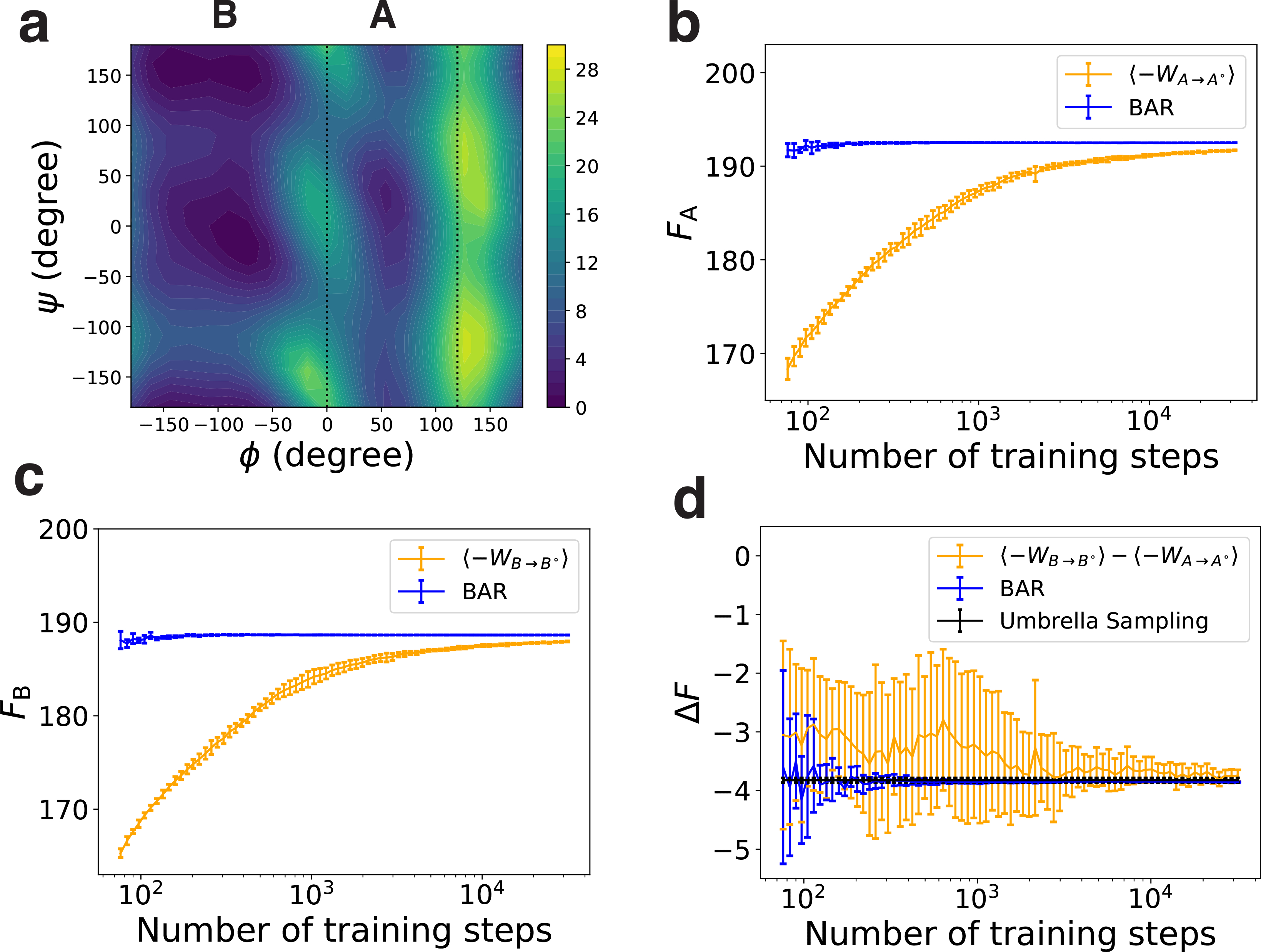
Performance of different free energy estimators on the di-alanine. Energy is shown in the units of k_BT. (a) Contour plot of the di-alanine free energy surface as a function of the two torsion angles ϕ and ψ. (b, c) The absolute free energy of state A and B computed with different estimators. (d) The free energy difference between state A and B computed with different estimators. Error bars representing one standard deviation are estimated using five independent repeats.

Figure 4:

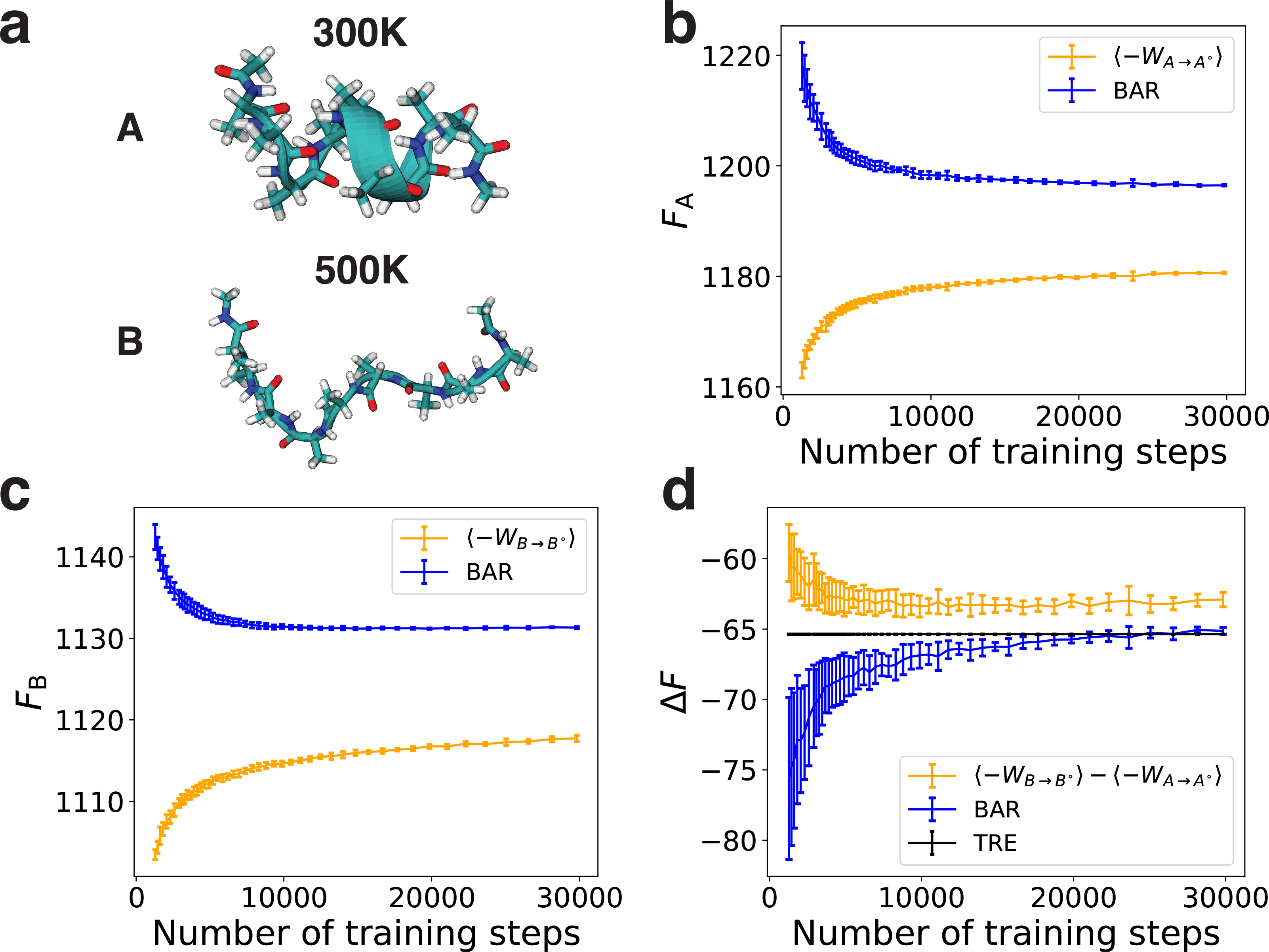
Performance of different free energy estimators on the deca-alanine. Energy is shown in the units of k_BT, with T = 300 K. (a) Representative conformations from state A (the ensemble at T = 300K) and state B (the ensemble at T = 500K). (b, c) The absolute free energy of states A and B computed with different estimators. (d) The free energy difference between states A and B computed with different estimators. Error bars representing one standard deviation are estimated using five independent repeats.

To compute the absolute free energy, we learned the reference states using normalizing flow based generative models.^39,45 Specifically, q_θ(x) was parameterized with multiple bijective transformations, T₁, ..., T_K, to convert a random variable u to a peptide configuration, i.e.,

$$x=T(u)=T_K\circ \cdots \circ T_1(u).$$ (8)

u shares the same dimension as x and is from a simple base distribution p_u(u). Based on the formula of variable change in probability density functions, we have

$$\ln q_{\theta }(x)=\ln p_u(u)-\sum _{k=1}^K\ln \left|J_{T_k}\left(u_{k-1}\right)\right|,$$ (9)

where u_k = T_k ± · · ·T₁(u₀) and $u_0=u.J_{T_k}$ is the Jacobian matrix of the transformation T_k, and | · | denotes the absolute value of the determinant. For both molecules, we first transformed u into the internal coordinates z based on moleculear topology (Fig. S1) and then transformed z into the Cartesian coordinates x using the neural spline flows^46,47 with coupling layers (Figs. S2 and S3).²⁵

The reference models were separately trained using configurations collected for each state from molecular dynamics simulations with the Amber ff99SB force field⁴⁸ and the OBC implicit solvent model.⁴⁹ As shown in Figs. S4–S7, they succeed in generating peptide conformations with reasonable geometry and energy. With the learned reference states, we computed the absolute free energy for states A and B using the three estimators. As shown in Figs. 3b, 3c, 4b and 4c, the BAR estimator converges much faster than the upper and lower bounds. The results calculated using the upper bound are not shown here because they are much larger than that of the lower bound and the BAR estimator (Figs. S8 and S9). Unlike the results for the SK model, the two bounds no longer converge to the same value or the BAR estimator, and their difference can be as large as 6 k_BT for di-alanine (Fig. S8) and 60 k_BT for deca-alanine (Fig. S9). The large gaps between the two bounds suggest that the generative models are still quite different from the true distributions even after the learning has converged. We expect the numbers from the BAR estimator to be correct, because the BAR estimator does not require the generative models to precisely match the original distributions to reproduce the free energy, as shown in both the Müller system and the SK model. Furthermore, the BAR estimations lie in between the two bounds in all four cases (Figs. S8 and S9), as expected for the exact values. Therefore, for these two molecular systems, the two bounds cannot be used for reliable estimation of the absolute free energy.

We further evaluated the accuracy of the three estimators in computing the free energy differences between states A and B. For comparison, we also determined the free energy difference using umbrella sampling³ for di-alanine and TRE simulations for deca-alanine. Results of estimated free energy differences are shown in Figs. 3d and 4d. The BAR estimator converges much faster to the results from umbrella sampling or TRE simulations than the two bounds. For di-alanine, the free energy difference estimated using BAR is −3.86 ± 0.01 k_BT, which agrees with the result from umbrella sampling (−3.82 ± 0.04 k_BT). To our surprise, the difference computed using the lower bound, −3.74 ± 0.10 k_BT, is close to the correct result as well. Because the lower bound is biased, we believe its good performance on the free energy difference is due to error cancellation. For deca-alanine, the free energy difference from TRE is −65.37 ± 0.02 k_BT, which deviates from the result obtained from the lower bound (−62.91 ± 0.52 k_BT) but agrees well the BAR estimation (−65.13 ± 0.23 k_BT).

CONCLUSION AND DISCUSSION

In summary, we demonstrated that the framework based on deep generative models succeeds at computing the absolute free energy using sample configurations from the state of interest and is applicable for both discrete and continuous systems. Compared with harmonic approximations¹⁸ or histograms²¹ used in previous methods to construct reference systems, deep generative models are more flexible and can capture the complex correlation among various degrees of freedom. Their flexibility is crucial for improving the overlap between the learned reference system and the state of interest and for ensuring the convergence of free energy estimations using the BAR method. Although the examples tested here are relatively small in size, the free energy calculation method can be readily applied to larger lattice models and more complex biomolecular systems in gas phase or implicit solvent.

Additional challenges must be addressed, however, before applying the proposed method to systems with explicit solvation. Similar to other techniques, ^50–56 the accuracy of computed free energy relies on the statistical convergence of conformational sampling, which can become more challenging with the presence of solvent molecules. Instead of collecting training data from unbiased molecular dynamics (MD) simulations, enhanced sampling methods such as solute tempering⁵⁷ may be necessary to improve the efficiency of configurational space exploration. In addition, including solvent molecules significantly increases the system size and introduces additional symmetry requirements for the generative models. While the issues with a larger system size can in principle be overcome with more powerful computers, efficiently encoding the permutational symmetry of solvent molecules into generative models’ architectures is less straightforward. It is worth noting that multiple studies^13,58,59 have introduced approaches for designing deep generative models that are invariant to permutations. Combining these approaches with our framework to compute the absolute free energy of biomolecular systems with explicit solvent would be an exciting direction for future studies. It could greatly facilitate the evaluation of protein-ligand binding affinity and protein conformational stability while accounting for entropic contributions.

References

- (1).Jorgensen WL The many roles of computation in drug discovery. Science 2004, 303, 1813–1818. [DOI] [PubMed] [Google Scholar]
- (2).Auer S; Frenkel D Prediction of absolute crystal-nucleation rate in hard-sphere colloids. Nature 2001, 409, 1020–1023. [DOI] [PubMed] [Google Scholar]
- (3).Torrie GM; Valleau JP Nonphysical sampling distributions in Monte Carlo free-energy estimation: Umbrella sampling. J. Comput. Phys 1977, 23, 187–199. [Google Scholar]
- (4).Kumar S; Rosenberg JM; Bouzida D; Swendsen RH; Kollman PA The weighted histogram analysis method for free-energy calculations on biomolecules. I. The method. J. Comput. Chem 1992, 13, 1011–1021. [Google Scholar]
- (5).Jorgensen WL; Ravimohan C Monte Carlo simulation of differences in free energies of hydration. J. Chem. Phys 1985, 83, 3050–3054. [Google Scholar]
- (6).Shirts MR; Chodera JD Statistically optimal analysis of samples from multiple equilibrium states. J. Chem. Phys 2008, 129, 124105. [DOI] [PMC free article] [PubMed] [Google Scholar]
- (7).Schneider E; Dai L; Topper RQ; Drechsel-Grau C; Tuckerman ME Stochastic neural network approach for learning high-dimensional free energy surfaces. Phys. Rev. Lett 2017, 119, 150601. [DOI] [PubMed] [Google Scholar]
- (8).Pohorille A; Jarzynski C; Chipot C Good practices in free-energy calculations. J. Phys. Chem. B 2010, [DOI] [PubMed] [Google Scholar]
- (9).Klimovich PV; Shirts MR; Mobley DL Guidelines for the analysis of free energy calculations. J. Comput. Aided Mol. Des 2015, [DOI] [PMC free article] [PubMed] [Google Scholar]
- (10).Kollman P Free energy calculations: applications to chemical and biochemical phenomena. Chem. Rev 1993, 93, 2395–2417. [Google Scholar]
- (11).Hahn AM; Then H Using bijective maps to improve free-energy estimates. Phys. Rev. E 2009, 79, 011113. [DOI] [PubMed] [Google Scholar]
- (12).Jarzynski C Targeted free energy perturbation. Phys. Rev. E 2002, 65, 5. [DOI] [PubMed] [Google Scholar]
- (13).Wirnsberger P; Ballard AJ; Papamakarios G; Abercrombie S; Racanière S; Pritzel A; Jimenez Rezende D; Blundell C Targeted free energy estimation via learned mappings. J. Chem. Phys 2020, 153, 144112. [DOI] [PubMed] [Google Scholar]
- (14).Ding X; Vilseck JZ; Hayes RL; Brooks CL Gibbs sampler-based λ-dynamics and Rao–Blackwell estimator for alchemical free energy calculation. J. Chem. Theory Comput 2017, 13, 2501–2510. [DOI] [PMC free article] [PubMed] [Google Scholar]
- (15).Zwanzig RW High-temperature equation of state by a perturbation method. i. non-polar gases. J. Chem. Phys 1954, 22, 1420–1426. [Google Scholar]
- (16).Bennett CH Efficient estimation of free energy differences from Monte Carlo data. J. Comput. Phys 1976, 22, 245–268. [Google Scholar]
- (17).Hoover WG; Gray SG; Johnson KW Thermodynamic properties of the fluid and solid phases for inverse power potentials. J. Chem. Phys 1971, 55, 1128–1136. [Google Scholar]
- (18).Frenkel D; Ladd AJ New Monte Carlo method to compute the free energy of arbitrary solids. Application to the fcc and hcp phases of hard spheres. J. Chem. Phys 1984, 81, 3188–3193. [Google Scholar]
- (19).Hoover WG; Ree FH Use of computer experiments to locate the melting transition and calculate the entropy in the solid phase. J. Chem. Phys 1967, 47, 4873–4878. [Google Scholar]
- (20).Amon LM; Reinhardt WP Development of reference states for use in absolute free energy calculations of atomic clusters with application to 55-atom Lennard-Jones clusters in the solid and liquid states. J. Chem. Phys 2000, 113, 3573–3590. [Google Scholar]
- (21).Ytreberg FM; Zuckerman DM Simple estimation of absolute free energies for biomolecules. J. Chem. Phys 2006, 124, 104105. [DOI] [PubMed] [Google Scholar]
- (22).Schilling T; Schmid F Computing absolute free energies of disordered structures by molecular simulation. J. Chem. Phys 2009, 131, 231102. [DOI] [PubMed] [Google Scholar]
- (23).Berryman JT; Schilling T Free energies by thermodynamic integration relative to an exact solution, used to find the handedness-switching salt concentration for DNA. J. Chem. Theory Comput 2013, 9, 679–686. [DOI] [PubMed] [Google Scholar]
- (24).Uria B; Côté M-A; Gregor K; Murray I; Larochelle H Neural autoregressive distribution estimation. J. Mach. Learn. Res 2016, 17, 1–37. [Google Scholar]
- (25).Dinh L; Sohl-Dickstein J; Bengio S Density Estimation Using Real NVP. 5th International Conference on Learning Representations, ICLR 2017, Toulon, France, April 24–26, 2017, Conference Track Proceedings. 2017. [Google Scholar]
- (26).Ding X; Vilseck JZ; Brooks CL Fast solver for large scale multistate Bennett acceptance ratio equations. J. Chem. Theory Comput 2019, 15, 799–802. [DOI] [PMC free article] [PubMed] [Google Scholar]
- (27).Wu D; Wang L; Zhang P Solving statistical mechanics using variational autoregressive networks. Phys. Rev. Lett 2019, 122, 80602. [DOI] [PubMed] [Google Scholar]
- (28).Li S-H; Wang L Neural network renormalization group. Physical review letters 2018, 121, 260601. [DOI] [PubMed] [Google Scholar]
- (29).Kullback S; Leibler RA On information and sufficiency. Ann. Math. Stat 1951, 22, 79–86. [Google Scholar]
- (30).Nicoli KA; Nakajima S; Strodthoff N; Samek W; Müller K-R; Kessel P Asymptotically unbiased estimation of physical observables with neural samplers. Phys. Rev. E 2020, 101, 023304. [DOI] [PubMed] [Google Scholar]
- (31).Cover TM; Thomas JA Elements of Information Theory; Wiley-Interscience: USA, 2006. [Google Scholar]
- (32).Noé F; Olsson S; Kohler J; Wu H Boltzmann generators: Sampling equilibrium states of many-body systems with deep learning. Science 2019, 365, eaaw1147. [DOI] [PubMed] [Google Scholar]
- (33).Wu H; Köhler J; Noé F Stochastic normalizing flows. arXiv preprint arXiv:2002.06707 2020, [Google Scholar]
- (34).Nicoli KA; Anders CJ; Funcke L; Hartung T; Jansen K; Kessel P; Nakajima S; Stornati P On estimation of thermodynamic observables in lattice field theories with deep generative models. arXiv preprint arXiv:2007.07115 2020, [DOI] [PubMed] [Google Scholar]
- (35).Shirts MR; Bair E; Hooker G; Pande VS Equilibrium free energies from nonequilibrium measurements using maximum-likelihood methods. Phys. Rev. Lett 2003, 91, 140601. [DOI] [PubMed] [Google Scholar]
- (36).Dempster AP; Laird NM; Rubin DB Maximum likelihood from incomplete data via the EM algorithm. J. Royal Stat. Soc 1977, 39, 1–22. [Google Scholar]
- (37).Müller K; Brown LD Location of saddle points and minimum energy paths by a constrained simplex optimization procedure. Theoret. Chim. Acta 1979, 53, 75–93. [Google Scholar]
- (38).Sherrington D; Kirkpatrick S Solvable model of a spin-glass. Phys. Rev. Lett 1975, 35, 1792–1796. [Google Scholar]
- (39).Papamakarios G; Nalisnick E; Rezende DJ; Mohamed S; Lakshminarayanan B Normalizing flows for probabilistic modeling and inference. arXiv preprint arXiv:1912.02762 2019, [Google Scholar]
- (40).Kingma DP; Salimans T; Jozefowicz R; Chen X; Sutskever I; Welling M In Advances in Neural Information Processing Systems 29; Lee DD, Sugiyama M, Luxburg UV, Guyon I, Garnett R, Eds.; Curran Associates, Inc., 2016; pp 4743–4751. [Google Scholar]
- (41).Papamakarios G; Pavlakou T; Murray I In Advances in Neural Information Processing Systems 30; Guyon I, Luxburg UV, Bengio S, Wallach H, Fergus R, Vishwanathan S, Garnett R, Eds.; Curran Associates, Inc., 2017; pp 2338–2347. [Google Scholar]
- (42).Huang C; Krueger D; Lacoste A; Courville AC Neural Autoregressive Flows. Proceedings of the 35th International Conference on Machine Learning, ICML 2018, Stockholmsmässan, Stockholm, Sweden, July 10–15, 2018. 2018; pp 2083–2092. [Google Scholar]
- (43).Kingma DP; Ba J Adam: A Method for Stochastic Optimization. 3rd International Conference on Learning Representations, ICLR 2015, San Diego, CA, USA, May 7–9, 2015, Conference Track Proceedings. 2015. [Google Scholar]
- (44).Paszke A; Gross S; Massa F; Lerer A; Bradbury J; Chanan G; Killeen T; Lin Z; Gimelshein N; Antiga L et al. In Advances in Neural Information Processing Systems 32; Wallach H, Larochelle H, Beygelzimer A, dAlché-Buc F, Fox E, Garnett R, Eds.; Curran Associates, Inc., 2019; pp 8026–8037. [Google Scholar]
- (45).Rezende DJ; Mohamed S Variational Inference with Normalizing Flows. Proceedings of the 32nd International Conference on Machine Learning, ICML 2015, Lille, France, 6–11 July 2015. 2015; pp 1530–1538. [Google Scholar]
- (46).Durkan C; Bekasov A; Murray I; Papamakarios G In Advances in Neural Information Processing Systems 32; Wallach H, Larochelle H, Beygelzimer A, dAlché-Buc F, Fox E, Garnett R, Eds.; Curran Associates, Inc., 2019; pp 7511–7522. [Google Scholar]
- (47).Rezende DJ; Papamakarios G; Racanière S; Albergo MS; Kanwar G; Shanahan PE; Cranmer K Normalizing flows on tori and spheres. arXiv preprint arXiv:2002.02428 2020, [Google Scholar]
- (48).Tian C; Kasavajhala K; Belfon KA; Raguette L; Huang H; Migues AN; Bickel J; Wang Y; Pincay J; Wu Q et al. ff19SB: Amino-acid-specific protein backbone parameters trained against quantum mechanics energy surfaces in solution. J. Chem. Theory Comput 2019, 16, 528–552. [DOI] [PMC free article] [PubMed] [Google Scholar]
- (49).Onufriev A; Bashford D; Case DA Exploring protein native states and large-scale conformational changes with a modified generalized born model. Proteins 2004, 55, 383–394. [DOI] [PubMed] [Google Scholar]
- (50).Wang L; Wu Y; Deng Y; Kim B; Pierce L; Krilov G; Lupyan D; Robinson S; Dahlgren MK; Greenwood J et al. Accurate and reliable prediction of relative ligand binding potency in prospective drug discovery by way of a modern free-energy calculation protocol and force field. J. Am. Chem. Soc 2015, 137, 2695–2703. [DOI] [PubMed] [Google Scholar]
- (51).Woo H-J; Roux B Calculation of absolute protein–ligand binding free energy from computer simulations. Proc. Natl. Acad. Sci. U.S.A 2005, 102, 6825–6830. [DOI] [PMC free article] [PubMed] [Google Scholar]
- (52).Chodera JD; Mobley DL; Shirts MR; Dixon RW; Branson K; Pande VS Alchemical free energy methods for drug discovery: progress and challenges. Curr. Opin. Struct. Biol 2011, 21, 150–160. [DOI] [PMC free article] [PubMed] [Google Scholar]
- (53).Shirts MR; Mobley DL; Chodera JD In Chapter 4 Alchemical Free Energy Calculations: Ready for Prime Time?; Spellmeyer D, Wheeler R, Eds.; Annual Reports in Computational Chemistry; Elsevier, 2007; Vol. 3; pp 41–59. [Google Scholar]
- (54).Knight JL; Brooks III CL λ-Dynamics free energy simulation methods. J. Comput. Chem 2009, 30, 1692–1700. [DOI] [PMC free article] [PubMed] [Google Scholar]
- (55).Hayes RL; Armacost KA; Vilseck JZ; Brooks III CL Adaptive landscape flattening accelerates sampling of alchemical space in multisite λ dynamics. J. Phys. Chem. B 2017, 121, 3626–3635. [DOI] [PMC free article] [PubMed] [Google Scholar]
- (56).Kong X; Brooks III CL λ-dynamics: A new approach to free energy calculations. J. Chem. Phys 1996, 105, 2414–2423. [Google Scholar]
- (57).Liu P; Kim B; Friesner RA; Berne B Replica exchange with solute tempering: A method for sampling biological systems in explicit water. Proc. Natl. Acad. Sci. U.S.A 2005, 102, 13749–13754. [DOI] [PMC free article] [PubMed] [Google Scholar]
- (58).Bender CM; Garcia JJ; O’Connor K; Oliva J Permutation invariant likelihoods and equivariant transformations. arXiv preprint arXiv:1902.01967 2019, [Google Scholar]
- (59).Köhler J; Klein L; Noé F Equivariant flows: sampling configurations for multi-body systems with symmetric energies. arXiv preprint arXiv:1910.00753 2019, [Google Scholar]
Associated Data
This section collects any data citations, data availability statements, or supplementary materials included in this article.