Abstract
In all countries the political decisions aim to achieve an almost stable configuration with a small number of new infected individuals per day due to Covid-19. When such a condition is reached, the containment effort is usually reduced in favor of a gradual reopening of the social life and of the various economical sectors. However, in this new phase, the infection spread restarts and, moreover, possible mutations of the virus give rise to a large specific growth rate of the infected people. Therefore, a quantitative analysis of the regrowth pattern is very useful. We discuss a macroscopic approach which, on the basis of the collected data in the first lockdown, after few days from the beginning of the new phase, outlines different scenarios of the Covid-19 diffusion for longer time. The purpose of this paper is a demonstration-of-concept: one takes simple growth models, considers the available data and shows how the future trend of the spread can be obtained. The method applies a time dependent carrying capacity, analogously to many macroscopic growth laws in biology, economics and population dynamics. The illustrative cases of France, Italy and United Kingdom are analyzed.
Keywords: Covid-19 spreading, Mathematical models, Macroscopic growth laws, Carrying capacity
1. Introduction
The pandemic spreading of the Coronavirus infection 2019 (COVID-19) (World Health Organization a World Health Organization b; Novel Coronavirus (D-) is forcing billion of people to live in isolation. The related economical degrowth is producing dramatic conditions for workers, trade and industry.
In all countries the political decisions aim to reduce the spreading and to achieve an almost stable configuration of coexistence with the disease, where a small number of new infected individuals per day is sustainable. In this new condition, the containment effort is usually reduced in favor of a gradual reopening of the social life and of the various economical sectors. Moreover, the possible virus mutations can give rise to more aggressive strain. Therefore, a new phase of the infectious spread starts: the so called phase 2 (Ph2).
In the Ph2 the evaluation of the regrowth of the infection diffusion is a complex problem: microscopic models require a coupled dynamics of the stakeholders, implying a strong model dependence and a large number of free parameters (Grassly & Fraser, 2008; Herzog and BlaizotNiel Hens, 2017; Pastor-Satorras et al., 2015; Blanchard et al., Kruger; Pluchinoet al., 2004; Walters et al., 2018). For example, the asymptomatic population has been estimated about ≤ 50 (Flaxman et al., 2020), ≃ 10 (Fenga), ≃ 3 − 4 (Lanteri et al., 2003; Tuite et al., 2020) times the symptomatic one and the simulation in the Italian report on the effects of the reopening on the National Health System is based on a stochastic epidemic model including the age dependence, the demographic structure, the heterogeneity of social contacts in different meeting places (home, school, work, public transportation, cultural activity, shop, bank, post office) and many work sub-sectors (public health, manufacturing, building, trade, …) (Comitato Tecnico Scientif).
On the other hand, complementary approaches, which outline the Covid-19 evolution in Ph2 in a model independent way, on the basis of macroscopic growth laws (with few parameters) are a useful tool for monitoring the regrowth of the spreading by collecting data after few days from the end of the lockdown or, in general, of the restarting phase.
In this paper we propose a method, based on macroscopic variables (Castorina & Blanchard, 2012; Castorina et al., 2003, 2006; Lanteri et al., 2003) and with no explicit reference to the underlying dynamics, which analyzes the quantitative consequences of the impairment of the constraints.
The starting point is the observation that the Covid-19 spreading, after an initial exponential increase and a subsequent small slowdown (which follows the Gompertz law (GL) (Gompertz, 1825) or other non linear trends), reaches a saturation, stable phase, described by the GL or by a logistic equation (LL) (Verhulst, 1838), after which the Ph2 starts.
The GL, initially applied to human mortality tables (i.e. aging), also describes tumor growth, kinetics of enzymatic reactions, oxygenation of hemoglobin, intensity of photosynthesis as a function of CO2 concentration, drug dose-response curve, dynamics of growth, (e.g., bacteria, normal eukaryotic organisms). The LL (Verhulst, 1838) has been used in population dynamics, in economics, in material science and in many other sectors.
The previous macroscopic growth laws, GL and LL, depend on two parameters, related to the initial exponential trend and to the maximum number of infected individuals, N∞, called carrying capacity.
It is well known that the carrying capacity changes according to some “external” conditions in many biological, economical and social systems (Meyer & Ausubel, 1999). In tumor growth it is related to a multi-stage evolution (Wheldon, 1988). In population dynamics, new technologies affect how resources are consumed, and since the carrying capacity depends on the availability of that resource, its value changes (Royama, 1992).
Therefore a simple method of monitoring the Ph2 is to understand how the carrying capacity (CC) increases due to the reduction of the social isolation, to the restarting of the economical activities and to more aggressive virus strains. As discussed, this modification is difficult to predict, but different scenarios of regrowth (i.e. with different time dependence of CC in the Ph2, for example) are analyzed in the next sections.
By monitoring the initial data in the new phase one outlines the behavior of the spreading for longer time to evaluate the possible effects of new mobility constraints or new total lockdown. If the infection regrows exponentially, the (re)lockdown and/or other containment efforts have to be decided as soon as possible. On the other hand, a small change of the specific rate in the Ph2, parameterized by a slight modification of the CC, should require less urgent political choices.
2. Theory and calculations
2.1. Macroscopic growth law with time dependent carrying capacity
The macroscopic growth laws for a population N(t) are solutions of a general differential equation that can be written as
| (1) |
where f(N) is the specific growth rate and its N dependence describes the feedback effects during the time evolution. If f(N) = constant, the growth follows an exponential pattern.
In particular, the Gompertz and the logistic equations are
| (2) |
| (3) |
where and kl are respectively the initial exponential rates and the other terms determine their slowdown. In both cases the steady state condition, dN/dt = 0 is reached when N is equal to the carrying capacity N∞.
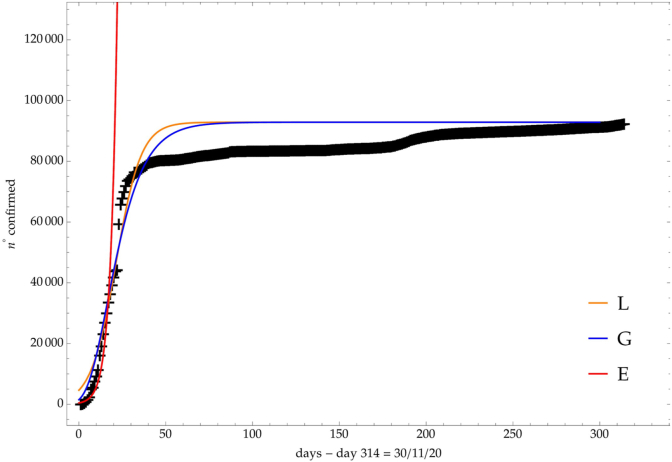
As shown in refs (Castorina et al., 2003; Lanteri et al., 2003). the coronavirus spreading has, in general, three phases: an initial exponential behavior, followed by a Gompertz one and a final logistic phase, due to lockdown. Fig. 1 for China shows exactly this time evolution and, indeed, in many dynamical systems the previous, simple, GL or LL solutions give a good quantitative understanding of the growth.
Fig. 1.
Comparison of the growth laws with the data of the cumulative number of infected individuals in China.
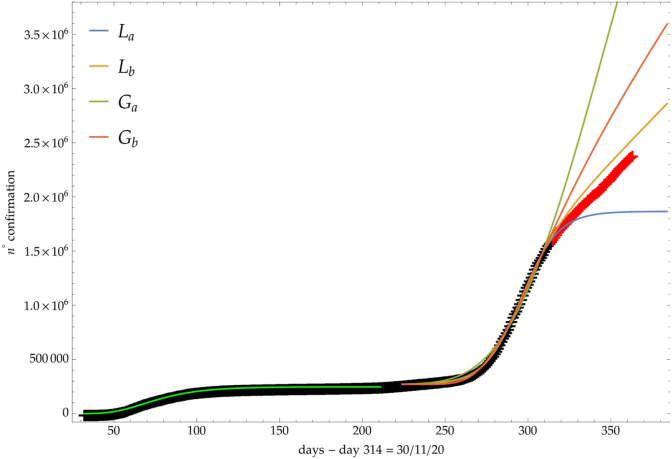
On the other hand, Fig. 2, where the number of infected people in Italy is depicted (see discussion below), shows a clear example of a Ph2 phase after the logistic steady phase.
Fig. 2.
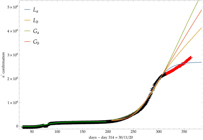
Comparison of the growth laws with the data of the cumulative number of infected individuals in Italy (see text below): data until 30th November (black), more recent data (red). Light-green curve is the GC fit of the first phase data. Data after November 30th (red points) are compared with the extrapolation of the fitted curves according to trends (a, b) of the CC.
Therefore, the CC (and in general, the macroscopic parameters describing the time evolution) can be modified by effects not included in eqs. (2), (3).
For example, the invention and diffusion of technologies lift the growth limit and the infectious diseases spread increases by human mobility and by possible genetic mutations.
Accordingly, one introduces an extension to the widely-used macroscopic model to allow for a time dependent carrying capacity and a change in the parameter which characterize the exponential initial phase, due to the different infectious features of the Covid-19. In other terms, eqs. (2), (3) are now respectively coupled with different values of the constant kg or kl and a differential equation for the evolution of the CC, i.e. (g = Gompertz, l = logistic)
| (4) |
where βg,l(t) are the rates: β = 0, β = constant, β ≃ tn, β ≃ c exp(b t) give respectively constant, linear, power law and exponential time dependence of the CC.
2.2. Covid-19 spreading in phase 2 - formulation and examples
The application of the previous differential equations to the spreading of Covid-19 in the Ph2 in different Countries requires: a) the time, t⋆, of the beginning of the change of the isolation conditions and/or of the restarting phase; b) a stable phase of the infection diffusion for t < t⋆: the effects of the political decision of reducing the constraints start (or should start) when the disease shows a clear slowdown (see below).
Therefore for t ≤ t⋆ the total number of infected individuals is described by eqs. (2), (3) with constant fitted by the available data, and for t ≥ t⋆ one has to solve the system of coupled differential equations (2), (3), (4) where the CC is a function of time, with the initial condition that .
A simple example is useful to outline the strategy. If a time t∗ the spread is stable, then and the specific rate is very small. Let us assume that for t > t∗ there is a fast rate of the spreading which follows the GL in the new phase with a new CC, i.e.
| (5) |
where is the carrying capacity in the new phase and N(t∗) is the initial value of the regrowth. If , with constant γ, the Gompertz equation for t > t∗ is given by
| (6) |
that is
| (7) |
and if a new exponential phase of the spread starts for t > t∗.
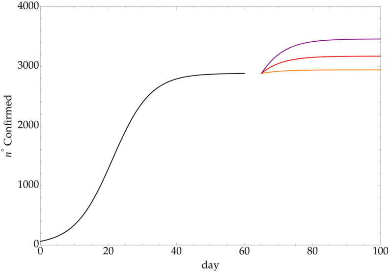
The condition t > t⋆ has to be better clarified. The instantaneous change of the CC is unphysical since there is a time interval to observe a possible increase of the spreading due to the Covid-19 incubation time, Δ. Therefore in the time interval t⋆ < t < t⋆ + Δ the growth behavior still follows the initial phase, with a fixed CC. The study of the incubation time is crucial to define the delay (after t⋆) of a possible regrowth. This aspect is discussed in the next section and to clarify the proposed method let us assume that a logistic trend up to t⋆ = 60 days, with a CC, , is modified at the day t⋆ = 60 + Δ, with Δ = 5, by an increase of the CC by a constant factor (1.02, 1.1, 1.20). Fig. 3 shows the cumulative number of detected infected individuals.
Fig. 3.
Variation of a logistic growth due to a sudden change in the CC: , with k = 1.02 (orange), k = 1.1 (red) and k = 1.2 (purple).
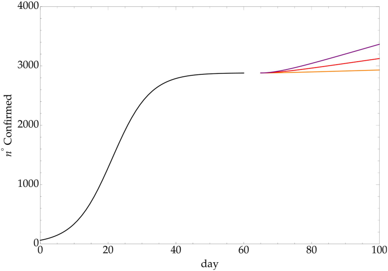
A weaker effect is obtained by considering a linear time dependence of the CC, i.e. N∞(t) = N∞(t⋆) + b [t − (60 + 5)] with b such that N∞(100) = 1.02, 1.1, 1.2 N∞(t⋆) respectively. The result is reported in fig. (4).
Fig. 4.
LL - linear time dependence CC, with and k = 1.02 (orange), k = 1.1 (red) and k = 1.2 (purple).
The previous examples are for illustrative purposes and in the next sections we apply the proposed approach to France, Italy and United Kingdom.
2.3. Covid-19 incubation time
The definition of the incubation time, or the time from infection to illness onset, is necessary to inform choices of quarantine periods, active monitoring, surveillance, control and modeling. COVID-19 emerged just recently, and the presence of a high rate of asymptomatic individuals, does not currently allow a precise estimation of incubation time. Different studies, especially at the beginning of the pandemic, tried to define the incubation period, obtaining a mean time varying between 4.0 and 6.4 days (Backer et al., 2020; Guan et al., 2020; Li et al., 2020).
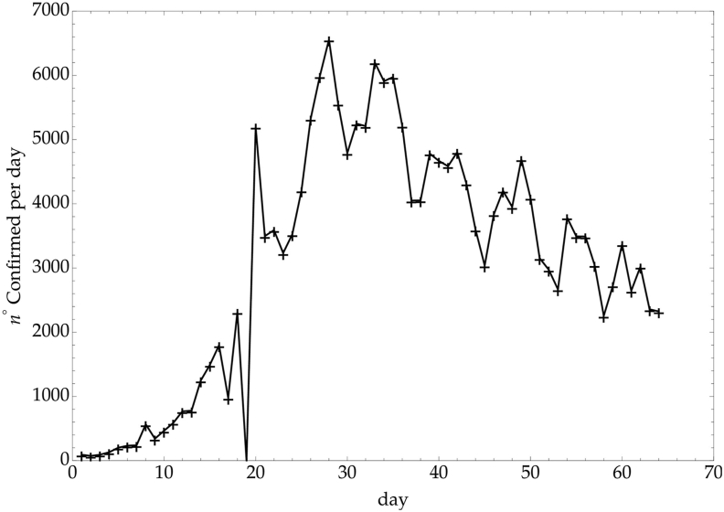
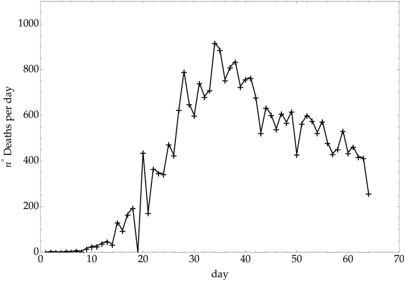
This value of incubation time is similar to other Coronaviruses, such as MERS-CoV and SARS-CoV, and generally accepted as a reliable estimate. However, 95% confidence intervals are large, varying from 2.4 days to 15.5 days (Backer et al., 2020). This strong variability is related to an uncertainty of the most probable date of exposure and onset of symptoms and this is the main reason why the WHO recommended an isolation time of 14 days after exposure to avoid more spreading of the infection (Lei et al., 2020). In our study, knowledge of the incubation time is necessary to model possible consequence of a re-opening. As a matter of fact, reduction of social isolation will increase the CC, and our attention should still be at its highest levels for at least two entire incubation periods, to promptly recognize any warning signal and apply the right control measures. Therefore the incubation time Δ ≃ 8 ± 6 days can be considered and Δ = 6 will be used in the next sections. Let us recall that an increase of Covid-19 mortality in Ph2 should be observed after a longer time interval. In Italy, for example, the correlation between the rate of infected people per day and the corresponding mortality rate shows a delay of about 8 days (see Fig. 5, Fig. 6). Therefore an increase of mortality could be expected after 14–22 days from t⋆.
Fig. 5.
Italy - Confirmed daily rate.
Fig. 6.
Italy - Mortality daily rate.
3. Results and discussion
The regrowth phase has been analyzed by two possible trends described by a LL/GL with carrying capacity:
-
a)
,
-
b)
,
where γ is a constant. In the next sections, Ga,b and La,b indicate the fits and the time evolution with the GL and LL, respectively, in the corresponding case a and b.
3.1. Phase 2 in Italy: possible scenarios
In the first phase, the Italian data followed the previously discussed three phases evolution (see Fig. 2). More recently, the Ph2 phase started and different regrowth scenarios will be outlined by an increase of the CC.
For the previous trends (a, b), Fig. 2 shows the comparison of the growth laws with the data of the cumulative number of confirmed infected individuals from February 2020, t∗ + Δ = 1th September 2020, to 30th November 2020 (black points). The curve extrapolation is then compared with data from November 30th onwards (red points) in such a way to verify the effective growth pattern in the new phase and to give some useful indications for political decisions.
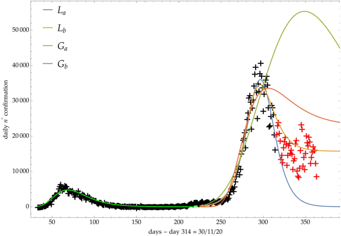
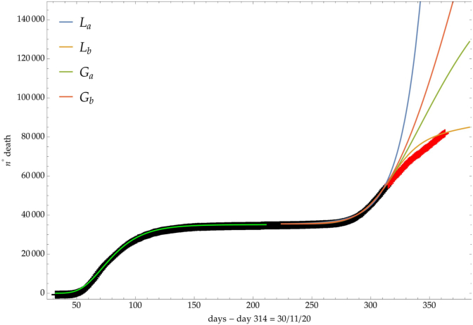
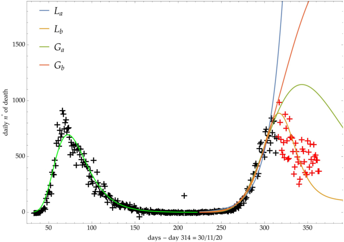
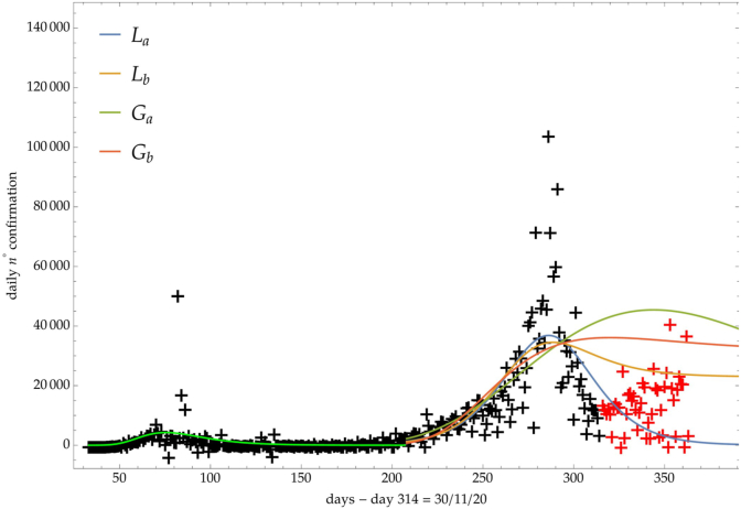
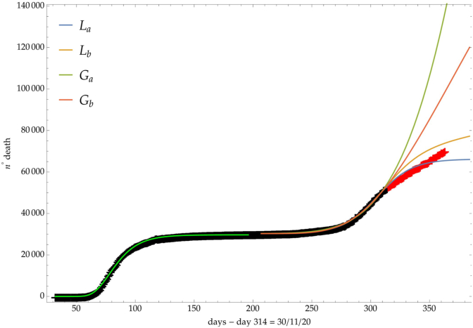
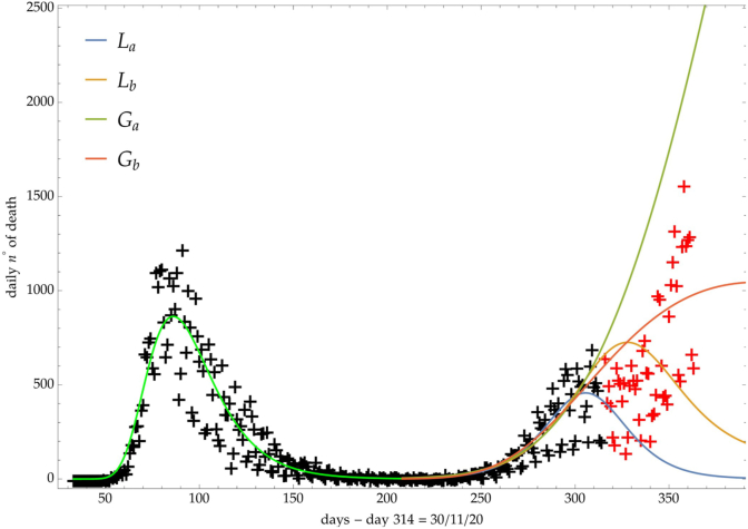
The same analysis is reported in Fig. 7, Fig. 8, Fig. 9 respectively for the daily number of confirmed infected individuals, for the cumulative number of deaths and for the daily number of deaths.
Fig. 7.
Italy: comparison of the growth laws with the data of the daily number of confirmed infected individuals from the initial day 22/Feb to the final day 30/Nov (black points). Light-green curve is the GC fit on the first phase data. Data after November 30th (red points) are compared with the extrapolation of the fitted curves according to trends (a, b) of the CC.
Fig. 8.
Italy: comparison of the growth laws with the data of the cumulative number of deaths from the initial day 22/Feb to the final day 30/Nov (black points). Light-green curve is the GC fit of the first phase data. Data after November 30th (red points) are compared with the extrapolation of the fitted curves according to trends (a, b) of the CC.
Fig. 9.
Italy: comparison of the growth laws with the data of the daily number of deaths from the initial day 22/Feb to the final day 30/Nov (black points). Light-green curve is the GC fit onfthe first phase data. Data after November 30th (red points) are compared with the extrapolation of the fitted curves according to trends (a, b) of the CC.
The effects of the mobility constraints decided by the italian government can be monitored by looking at the different predicted trends.
3.2. France
France is in a phase of strong spread of the virus, started in August 2020, with an almost total lockdown.
As in the previous case, Fig. 10, Fig. 11, Fig. 12, Fig. 13 are devoted to the comparison of the growth laws with the data from February to November the 30th (black points) 2020 of the cumulative number of confirmed infected individuals, of the daily number of confirmed infected individuals, of the total and daily number of deaths. Analogously to the previous discussion for Italy, the extrapolation of the fitted curves after November 30th gives important information for the more recent time evolution of the Covid-19 spread.
Fig. 10.
France: comparison of the growth laws with the data of the confirmed infected individuals from the initial day 22/Feb to the final day 30/Nov (black points). Light-green curve is the GC fit of the first phase data. Data after November 30th (red points) are compared with the extrapolation of the fitted curves according to trends (a, b) of the CC.
Fig. 11.
France: comparison of the growth laws with the data of the daily number of confirmed infected individuals from the initial day 22/Feb to the final day 30/Nov (black points) 2020. Light-green curve is the GC fit of the first phase data. Data after November 30th (red points) are compared with the extrapolation of the fitted curves according to trends (a, b) of the CC.
Fig. 12.
France: comparison of the growth laws with the data of the cumulative number of deaths from the initial day 22/Feb to the final day 30/Nov (black points). Light-green curve is the GC fit of the first phase data. Data after November 30th (red points) are compared with the extrapolation of the fitted curves according to trends (a, b) of the CC.
Fig. 13.
France: comparison of the growth laws with the data of the daily number of deaths from the initial day 22/Feb to the final day 30/Nov (black points). Light-green curve is the GC fit of the first phase data. Data after November 30th (red points) are compared with the extrapolation of the fitted curves according to trends (a, b) of the CC.
3.3. United Kingdom
Very recently in United Kingdom (UK) a new phase of very fast spread of Covid-19 started.
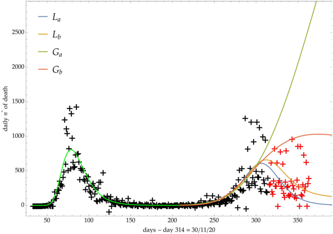
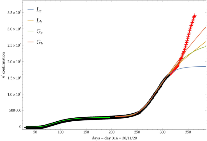
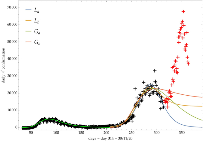
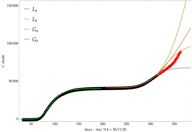
Differently from Italy and France, where the Ph2 is mainly due to weaker constraints on mobility and on social aggregation, in UK the fast growth of the specific spread rate is related to a Covid-19 mutation, with a more dangerous strain.
This condition is immediately seen in Fig. 14, Fig. 15, Fig. 16, Fig. 17 respectively for the cumulative number of confirmed infected individuals, of the daily number of confirmed infected individuals, of the total and daily number of deaths. After fitting the data from February 2020 to 30th November 2020, there is no agreement with the extrapolated curves for a constant increase (trend a) or a linear time growth (trend b) of the CC both for GL and LL.
Fig. 14.
UK: comparison of the growth laws with the data of the cumulative number of confirmed infected individuals from the initial day 22/Feb to the final day 30/Nov (black points). Light-green curve is the GC fit of the first phase data. Data after November 30th (red points) are compared with the extrapolation of the fitted curves according to trends (a, b) of the CC.
Fig. 15.
UK: comparison of the growth laws with the data of the daily number of confirmed infected individuals from the initial day 22/Feb to the final day 30/Nov (black points). Light-green curve is the GC fit of the first phase data. Data after November 30th (red points) are compared with the extrapolation of the fitted curves according to trends (a, b) of the CC.
Fig. 16.
UK: comparison of the growth laws with the data of the cumulative number of deaths from the initial day 22/Feb to the final day 30/Nov (black points). Light-green curve is the GC fit of the first phase data. Data after November 30th (red points) are compared with the extrapolation of the fitted curves according to trends (a, b) of the CC.
Fig. 17.
UK: comparison of the growth laws with the data of the daily number of deaths from the initial day 22/Feb to the final day 30/Nov (black points). Light-green curve is the GC fit of the first phase data. Data after November 30th (red points) are compared with the extrapolation of the fitted curves according to trends (a, b) of the CC.
The effect is clear in the daily number of confirmed infected also, where the very recent lockdown political decision is now producing a decreasing behavior.
4. Comments and conclusions
The purpose of this paper is a demonstration-of-concept: one takes simple growth models, considers the available data and shows different scenarios of the future trend of the spreading. The method applies a time dependent carrying capacity since the reduction of containment efforts and/or virus mutations change this crucial parameters of the macroscopic growth laws. Different time behaviors of the CC outline various trends in the new phase, with clear evidence of the regrowth pattern due to weaker social constraint with respect to more dangerous virus strains.
Therefore a comparison of data, collected in a short time interval, with the plots obtained by the various ansatz for the CC can help to decide if the social isolation conditions have to be strengthened or weakened and can signal a new virus mutation. Finally, a large variation of the CC signals an increase of the pressure on the National Health systems.
Handling Editor: Dr. J Wu
Footnotes
Peer review under responsibility of KeAi Communications Co., Ltd.
References
- Backer J.A., Klinkenberg D., Wallinga J. Incubation period of 2019 novel coronavirus (2019-nCoV) infections among travellers from Wuhan, China, 20-28 January 2020. Euro Surveillance. 2020;25(5) doi: 10.2807/1560-7917.ES.2020.25.5.2000062. [DOI] [PMC free article] [PubMed] [Google Scholar]
- P. Blanchard, G. F. Bolz and T. Kruger, Mathematical modelling on random graphs of sexually trasmitted disease, in Dynamics and stochastic process - theory and applications, lecture notes in physics, vol. Vol. 355, Springer-Verlag, Berlin.
- Castorina P., Blanchard P. Unified approach to growth and aging in biological, technical and biotechnical systems. SpringerPlus. 2012;1:7. doi: 10.1186/2193-1801-1-7. [DOI] [PMC free article] [PubMed] [Google Scholar]
- Castorina P., Delsanto P.P., Guiot C. Classification scheme for phenomenological universalities in growth problems in physics and other sciences. Physical Review Letters. 2006;96:188701. doi: 10.1103/PhysRevLett.96.188701. [DOI] [PubMed] [Google Scholar]
- Castorina P., Lanteri D., Iorio A. Data analysis on Coronavirus spreading by macroscopic growth laws. International Journal of Modern Physics C. 2003 in press in. arXiv. [Google Scholar]
- Comitato Tecnico Scientifico, Italian Government ( in Italian).
- L.Fenga, CoViD19: An Automatic,Semiparametric estimation method for the population infected in Italy, medRxiv preprint. [DOI] [PMC free article] [PubMed]
- Flaxman Seth, Mishra Swapnil, Gandy Axel. Imperial College London; 2020. Estimating the number of infections and the impact of non- pharmaceutical interventions on COVID- 19 in 11 European countries. [Google Scholar]
- Gompertz B. On the nature of the function expressive of the law of human mortality and a new mode of determining life contingencies. Phil. Trans. R. Soc. 1825;115:513. [Google Scholar]
- Grassly N.C., Fraser C. Mathematical models of infectious disease transmission. Nature Reviews Microbiology. 2008;6:477. doi: 10.1038/nrmicro1845. [DOI] [PMC free article] [PubMed] [Google Scholar]
- Guan W.-J. Clinical characteristics of coronavirus disease 2019 in China. New England Journal of Medicine. February 2020 doi: 10.1056/NEJMoa2002032. [DOI] [PMC free article] [PubMed] [Google Scholar]
- Herzog S.A., Blaizot S., Niel Hens Mathematical models used to inform study design or surveillance systems in infectious diseases: A systematic review. BMC Infectious Diseases. 2017;17:775. doi: 10.1186/s12879-017-2874-y. [DOI] [PMC free article] [PubMed] [Google Scholar]
- Lanteri D., Carco’ G., Castorina P. How macroscopic laws describe complex dynamics: Asymptomatic population and CoviD-19 spreading. International Journal of Modern Physics C. 2003:12457. in press in. arXiv. [Google Scholar]
- Lei S. Clinical characteristics and outcomes of patients undergoing surgeries during the incubation period of COVID-19 infection. EClinicalMedicine. April 2020:100331. doi: 10.1016/j.eclinm.2020.100331. [DOI] [PMC free article] [PubMed] [Google Scholar]
- Li Q. Early transmission dynamics in Wuhan, China, of novel coronavirus-infected pneumonia. New England Journal of Medicine. 2020;382(13):1199–1207. doi: 10.1056/NEJMoa2001316. [DOI] [PMC free article] [PubMed] [Google Scholar]
- Meyer P.S., Ausubel J.H. Carrying capacity: A model with logistically varying limits. Technological Forecasting and Social Change. 1999;61(3):209–214. [Google Scholar]
- Novel coronavirus (COVID-19) cases, provided by JHU CSSE.
- Pastor-Satorras R., Castellano C., Van Mieghem P., Vespignani A. Epidemic processes in complex network. Reviews of Modern Physics. 2015;87 [Google Scholar]
- Pluchino A. 2004. A Novel methodology for epidemic Risk Assessment: The case of COVID-19 outbreak in Italy. arXiv. 02739. [Google Scholar]
- Royama T. Springer ed. 1992. Analytical population dynamics. [Google Scholar]
- Tuite A.R., Ng V., Rees E., Fisman D. Estimation of COVID-19 outbreak size in Italy. The Lancet Infectious Diseases. 2020 doi: 10.1016/S1473-3099(20)30227-9. Published Online March 19, 2020. [DOI] [PMC free article] [PubMed] [Google Scholar]
- Verhulst P.F. Notice sur la loi que la population poursuit dans son accroissement. Correspondance Mathématique et Physique. 1838;10:113. [Google Scholar]
- Walters C.E., Mesle’ M.I., Hall I.M. Modelling the global spread of diseases: A review of current practice and capability. Epidemics. 2018;25:1. doi: 10.1016/j.epidem.2018.05.007. [DOI] [PMC free article] [PubMed] [Google Scholar]
- Wheldon T.E. Adam Hilger; 1988. Mathematical model in cancer Research. [Google Scholar]
- World Health Organization, Coronavirus disease (COVID-19) outbreak.
- World Health Organization, reportCoronavirus disease (COVID-19), China joint mission on covid 19 final report.


