Measuring differences between phenomenological growth models applied to epidemiology

Abstract

Phenomenological growth models (PGMs) provide a framework for characterizing epidemic trajectories, estimating key transmission parameters, gaining insight into the contribution of various transmission pathways, and providing long-term and short-term forecasts. Such models only require a small number of parameters to describe epidemic growth patterns. They can be expressed by an ordinary differential equation (ODE) of the type $C^{\prime }\left(t\right)=f(t,C;\Theta )$ for $t>0$, $C\left(0\right)=C_0$, where $t$ is time, $C\left(t\right)$ is the total size of the epidemic (the cumulative number of cases) at time $t$, $C_0$ is the initial number of cases, $f$ is a model-specific incidence function, and $\Theta$ is a vector of parameters. The current COVID-19 pandemic is a scenario for which such models are of obvious importance. In Bürger et al. (2019) it is demonstrated that some PGMs are better at fitting data of specific epidemic outbreaks than others even when the models have the same number of parameters. This situation motivates the need to measure differences in the dynamics that two different models are capable of generating. The present work contributes to a systematic study of differences between PGMs and how these may explain the ability of certain models to provide a better fit to data than others. To this end a so-called empirical directed distance (EDD) is defined to describe the differences in the dynamics between different dynamic models. The EDD of one PGM from another one quantifies how well the former fits data generated by the latter. The concept of EDD is, however, not symmetric in the usual sense of metric spaces. The procedure of calculating EDDs is applied to synthetic data and real data from influenza, Ebola, and COVID-19 outbreaks.

1. Introduction

1.1. Scope

A wide variety of mathematical models have been used to study the patterns of growth processes of populations and epidemics in humans, animals, and plants [1], [2], [3], [4], [5], [6], [7], [8], [9], [10], [11], [12], [13], [14]. Here we are especially interested in dynamic growth models for characterizing epidemic trajectories, estimating key transmission parameters, gaining insight into the contribution of various transmission pathways, and providing long-term and short-term forecasts. The recent monograph by Yan and Chowell [15] provides an introduction to the topic. We herein focus on phenomenological growth models (PGMs) that only require a small number of parameters are commonly used to describe epidemic growth patterns, and which can be expressed by an ordinary differential equation (ODE) of the type

$$C^{\prime }\left(t\right)≔\frac{\mathrm{d}C\left(t\right)}{\mathrm{d}t}=f(t,C;\Theta ),t>0;C\left(0\right)=C_0,$$ (1.1)

where $t$ is time, $C\left(t\right)$ is the total size of the epidemic (the cumulative number of cases) at time $t$, $C_0$ is the initial number of cases, $f$ is an incidence function that is specific to each PGM under study, and $\Theta$ is a vector of parameters. Such models have been used to study the epidemics of influenza [16], [17], [18], Ebola [19], [20], [21], [22], Zika [23], [24], [25], Chikungunya [26], and others of global interest. The current COVID-19 pandemic is a scenario for which such models are of obvious importance [27], [28], [29], [30], [31], [32], [33], [34].

In [16] we demonstrate that some models are better at fitting data of specific epidemic outbreaks than others even when the models have the same number of parameters. Consider, for instance, the three-parameter so-called generalized logistic model (GLM) specified by

$$f(t,C;\Theta )=rC{\left(t\right)}^p\left(1-C\left(t\right)∕K\right),\Theta =(r,p,K),$$ (1.2)

where the parameter $r>0$ indicates the growth rate (its dimension is $1∕\mathrm{time}$), $K$ is the size of the epidemic, and $p\in [0,1]$ is a growth scaling parameter that indicates the kind of growth (e.g., exponential vs. sub-exponential). In the comparative analysis between two models and their generalizations [16], the GLM was able to capture the trajectories for 37 real datasets describing the progression of epidemic outbreaks. In fact, this model showed to have the smallest error between the data and the fit, and the estimated parameters were identifiable, that is, the average value of each parameter was effectively a central value in the confidence intervals, where we used the definitions and calculations introduced in [35] for the error and the confidence intervals.

Although several PGMs could be considered for a given dataset, little work has been conducted to analyze the differences between models. Here we define the empirical directed distance between two PGMs as a measure of differences in the dynamics that each model is capable of generating. We address questions such as whether the dynamics of the logistic growth model (LM), defined by

$$f(t,C;\Theta )=rC\left(t\right)\left(1-C\left(t\right)∕K\right),\Theta =(r,K),$$ (1.3)

is more similar to that of the Gompertz model (GoM), corresponding to

$$f(t,C;\Theta )=rC\left(t\right)exp(-bt),\Theta =(r,b),$$ (1.4)

where the parameter $b>0$ describes the exponential decay of the growth rate $r$, or to that of the Richards model (RM)

$$f(t,C;\Theta )=rC\left(t\right)\left(1-{(C\left(t\right)∕K)}^p\right),\Theta =(r,K,p).$$ (1.5)

We emphasize that we use the terminologies “generalized logistic model” (GLM) and “Richards model” (RM) to address different models, namely those given by (1.2), (1.5), respectively. Only the model (1.5) is the one proposed originally in Richards’ paper [4]. That said, we are well aware that in parts of the literature, for instance in [36], [37], [38], the model (1.5) is referred to as “a generalized logistic model” (cf., e.g., [37]), that is “generalized logistic” and “Richards model” are used synonymously. We recall that our equation (1.2) is a generalization of the logistic model (1.3) where the exponent $p$ is applied to the first factor $C\left(t\right)$ in (1.3), while the Richards model (1.5) represents a different generalization that arises from applying an exponent $p$ to $C\left(t\right)∕K$ within the growth-limiting factor $1-C\left(t\right)∕K$.

Before proceeding, we comment that it is arguable whether in the context of epidemiology the scalar ODE (1.1) is really a phenomenological model or simply a generator of functions to be fitted to the available data. Strictly speaking only the LM can be viewed as an epidemiological model since it arises from the well-known susceptible–infectious (SI) compartmental model in the absence of births and deaths (see, e.g., [8]). However, the use of the word ‘model’ for (1.1) is not only very common in the epidemiological literature (including [1], [5], [16], [19], [20], [21], [23], [30], [31], [35] of the references cited so far), but we also mention that the various parameters carry relevant information characterizing the strength of an epidemic outbreak, much in contrast, say, to abstract coefficients of a function (e.g., spline function) to approximate data. That said, we emphasize that the approach of the present work is one of statistics applied to medicine and biology, and is independent of what one regards to be the ‘true’ status of (1.1).

There is a need to develop a methodology that helps quantify the differences in the dynamics obtained from different models that aim to capture growth processes in the social and natural sciences. Such a methodology can be helpful to assess which models are more parsimonious than others in different contexts. In the context of epidemic modeling, many models have been developed to investigate the transmission dynamics and control of infectious diseases [10], [14], [39]. However, there has not been a systematic study of differences between models and how differences in dynamics may explain the ability of certain models to provide a better fit to data than others. Here we aim to make progress in this direction by focusing on simple models that strive to capture many of the empirical patterns found in epidemic data. The main practical reason why one would be interested in understanding the distance between models stems from the need to understand how different the solutions from different models are. If two models are able to reproduce the same temporal dynamics, the researcher would be better off relying on the simpler model. Because a number of PGMs exist in the literature, we argue that understanding their differences in terms of the dynamics that they can produce adds to the literature and will help guide researchers in different applied disciplines select a reasonably small set of models rather than considering a large set of models many of which produce very similar results or fits to the data.

To address these questions we measure the differences in the dynamics between different dynamics models of the form (1.1). Here we employ simulated data for three generalized growth models (namely GLM, GGoM and RM), and with the help of mathematical and computational methods we calculate the fit and performance errors in terms of which the empirical directed distances (EDDs) are defined. As we will show, it turns out that the GLM is closer to the dynamics of the RM. On the other hand, the generalized Gompertz model (GGoM) defined by

$$f(t,C;\Theta )=rC{\left(t\right)}^{p}exp(-bt),\Theta =(r,b,p).$$ (1.6)

is the farthest from the RM and GLM. This is because the scaling parameter ($p$ in (1.2), (1.5), (1.6)) plays a more significant role in the GLM since its variation within the GLM causes more changes in its dynamics than for the other models.

The EDD between two PGMs, say $A$ and $B$, is based on simulation study that we introduce in the following sections. As the foregoing discussion shows, the word “distance” in this work is not to be understood in the mathematical sense as distance function on a metric space; rather, we employ it to characterize a measure of distance based on the mean squared error. The terminology of “distance measure between models” has been employed elsewhere, cf., e.g., [40].

1.2. Related work

To illustrate how models can support different features of epidemic data, we can refer to the scaling of epidemic growth that characterizes the early growth dynamics of epidemics. While some epidemics spread rapidly through a population following an exponential growth phase such as pandemic influenza or the ongoing epidemic of the novel coronavirus emerging from China (COVID-19) [27], some outbreaks spread more slowly as a result of the mode of transmission or the contact network through which the pathogen spreads. For instance, sexually transmitted diseases and Ebola do not spread through the air, but require a specific type of intimate contact to spread. In such situations the disease is expected to spread follow sub-exponential growth patterns. When a model only supports exponential growth dynamics, we could expect differences between such a model and more flexible models that can capture a range of early epidemic growth dynamics  [41].

The authors’ interest in PGMs is mainly motivated by epidemiological applications, where the quantity that grows is usually the size of the population of infected humans. The same models also arise in quite different contexts. In fact, PGMs are commonly used in fields such as mathematical oncology and population dynamics because they consider in a simple but (up tome extent and depending on the applications) effective way phenomena concerning the growth of cells or of animal or human populations. In other words these models mirror in a simple way phenomena pertaining to these population growth phenomena. In particular they are utilized to describe the growth of a tumor where $C\left(t\right)$ is proportional to the number of cells in the tumor. We refer to textbook entries, e.g. [42, Ch. 6], [43, Sect. 1.8], [44, p. 39], and [8, Sect. 8.2], the monograph by T.E. Wheldon [45], as well as some classic references cited in most of these works such as Aroesty et al. [46] and Newton [47]. In particular, in the latter two works it is demonstrated that the Gompertz model (1.4), under suitable choices of $r$ and $b$, agrees remarkably well with data on tumor growth as long as $C$ is not too small (as is pointed out in [42], [44]). More recent contributions that study, and compare, the applicability of various PGMs to tumor growth include [36], [37], [38], [48], [49].

One important step in our treatment consists in generating a fit of one of the PGMs to data that are either generated by another model or using real outbreak data. Since the parametric forms of PGMs are essentially non-linear, standard least-squares methods are often not applicable. Thus, to provide these fits, we resort to the Simulated Annealing (SA) method. This method is defined in [50] as a powerful stochastic search method applicable to a wide range of problems that occur in a variety of disciplines including physics, engineering problems, mathematical programming, and statistics. In particular, in the context of epidemiological models, SA has been applied to devise optimal time-profiles of public health intervention to shape voluntary vaccination for childhood diseases, see Buonomo et al. [51].

The problem can be formulated as follows. Suppose we are given finite-dimensional solution space $\mathcal{S}$, and a function $f:\mathcal{S}\to \mathbb{R}$, and we want find an optimal configuration $x^{\ast }\in \mathcal{S}$ such that $f\left(x^{\ast }\right)={min}_{x\in \mathcal{S}}f\left(x\right)$. This method has become very popular because the algorithm can solve unconstrained and bound-constrained optimization problems, especially in the multidimensional case when the objective function may have many local extremes and may not be smooth. In that case, SA is advantageous because it does not require calculation of derivatives, and thus be considered as a derivative-free method. In papers including [52], [53] this method has been used for parameter estimation, which motivated our computation.

1.3. Outline of the paper

In the next sections we define the PGMs considered in our study as well as the numerical method for parameter estimation and the quantification of the distance between two models. The concept of empirical directed distance (EDD) from one PGM to another is detailed in Section 2. To this end we summarize in Section 2.1 properties of the models under consideration and recall explicit solutions wherever available. Then, in Section 2.2 we outline the procedure to measure the EDD from a phenomenological growth model $B$ to another phenomenological growth model $A$, denoted by $EDD(B\to A)$, which we summarize in Algorithm 2.1. A crucial role within this algorithm is played by the SA method (utilized to find the optimal parameters for model $B$ when fitting a dataset generated by model $A$), which is briefly discussed in Section 2.3. Next, in Section 3 we apply the methodology to four models: LM, GLM, RM (with logistic growth) and GGoM introduced in Section 1.1 considering synthetic datasets (as outlined in Section 2.2). Specifically, we introduce in Section 3.1 the parameters and solution spaces for each of these models, with special emphasis on the exponent $p$. The specific application of the SA method is discussed in Section 3.2. Then, in Sections 3.3, 3.4, 3.5, 3.6 we present Experiments 1, 2, 3, and 4 in which we calculate distances from the LM, RM, GLM, and GGoM to other models, respectively. In Section 4 we apply the methodology to real data of outbreaks of influenza, Ebola, and COVID-19. Some conclusions are collected in Section 5.

2. Distance between phenomenological growth models

2.1. Notation and solution of PGMs

We begin the discussion with a comment on notation. The notation chosen for the incidence function $f=f(t,C;\Theta )$ presupposes that $t$ and $C$ are independent arguments. In fact, it is also possible to rewrite all models utilized herein as autonomous ordinary differential equations of the form

$$C^{\prime }\left(t\right)=\phi (C;\Theta ),t>0;C\left(0\right)=C_0.$$ (2.1)

This is directly obvious for the GLM (1.2) and the RM (1.5). Rewriting the ODEs for the GoM and GGoM (with $0<p<1$) as

$$exp(-b\tau )=\frac{1}{r}\frac{\mathrm{d}}{\mathrm{d}\tau }lnC\left(\tau \right)\text{and}exp(-b\tau )=\frac{1}{r(1-p)}\frac{\mathrm{d}}{\mathrm{d}\tau }{C}^{1-p}\text{for }0\le \tau \le t\text{,}$$

integrating with respect to $\tau$, and substituting the corresponding expression for $exp(-bt)$ in (1.4), (1.6), respectively, one obtains

$$\phi (C;\Theta )=\left(r+bln{C}_0\right)C-bClnC$$

for the GoM and

$$\phi (C;\Theta )=C^p\left(\frac{b}{p-1}\left(C^{1-p}-C_0^{1-p}\right)+r\right),0<p<1,$$

for the GGoM. The original and autonomous forms, (1.1), (2.1), are of course equivalent in all cases. However, one or another form is preferable depending on the context of application of the respective PGM, that is, on whether dependence of the growth rate on time or on the current size of population should be emphasized. For instance, as is pointed out in [46], in the application to tumor growth it considered more suggestive to relate the specific growth rate for a particular tumor to its size. On the other hand, in the application to epidemiological data we wish to compare model curves to given time series of data. Furthermore, we prefer a formulation that allows one to include explicit time dependence of the incidence rate by external factors at a later stage. One such external factor could be, for example, the seasonal variation of temperature. As compromise between these different viewpoints, we have chosen the dependence $f=f(t,C;\Theta )$. Finally, we mention that additional insight and comparison between different models can also be achieved from considering the population size and its growth rate as separate state variables and analyzing the fixed points and stability of the resulting dynamical system of two scalar equations, as is done e.g. in [48]. For instance, the GGoM (1.6) can be written as the coupled system $C^{\prime }=a{C}^p$, $a^{\prime }=-ba$ with the initial conditions $C\left(0\right)=C_0$, $a\left(0\right)=r$.

For the growth models summarized in Table 1, $p=0$ corresponds to a constant incidence over time, $p=1$ corresponds to exponential growth, and any intermediate value $0<p<1$ leads to a model that describes initial sub-exponential growth dynamics [41], [54], [55], [56]. In fact, in prior work we have demonstrated that some epidemics are characterized by early slower-than-exponential growth using flexible phenomenological models (see [54], [55]).

Table 1.

Summary of information on models and parameters.

Phenomenological growth model	Parameters
Logistic growth model (LM)	$\Theta =({\theta }_1=r,{\theta }_2=K);r,K>0$
Generalized Logistic growth model (GLM)	$\Theta =({\theta }_1=r,{\theta }_2=K,{\theta }_3=p);r,K>0,p\in [0,1]$
Richards model (RM)	$\Theta =({\theta }_1=r,{\theta }_2=K,{\theta }_3=p);r,K>0,p\in [0,1]$
Generalized Gompertz model (GGoM)	$\Theta =\{{\theta }_1=r,{\theta }_2=b,{\theta }_3=p\};r,b>0,p\in [0,1]$

Three of these models have an initial logistic growth because when $p=1$ for the GLM and RM, in other words the LM is recovered. In contrast, this is not the case for the GGoM. (The RM and GLM show two forms of incorporating the parameter $p$ to the LM model to obtain the generalized growth form $r{C}^p\left(t\right)$.) We wish to measure how close the logistic models are to each other and to the GGoM, and to assess whether two or three parameters are sufficient to recover other dynamics. We recall the following explicit solutions. The solution of the LM (1.1), (1.3) is given by

$$C\left(t\right)=\frac{KC\left(0\right)exp\left(rt\right)}{K+C\left(0\right)(exp\left(rt\right)-1)},$$ (2.2)

that of the GoM (1.1), (1.4) (that is, the GGoM for $p=1$) by

$$C\left(t\right)=C\left(0\right)exp\left((r∕b)\left(1-exp(-bt)\right)\right),$$ (2.3)

while for the GGoM (1.1), (1.4) we get

$$C\left(t\right)={\left((1-p)(r∕b)\left(1-exp(-bt)\right)+C{\left(0\right)}^{1-p}\right)}^{1∕(1-p)}\text{(where }0<p<1\text{).}$$ (2.4)

The solution of the RM (1.1), (1.5) is

$$C\left(t\right)=\frac{KC\left(0\right)exp\left(rt\right)}{{(K^p+C{\left(0\right)}^p(exp\left(prt\right)-1))}^{1∕p}}.$$ (2.5)

As is pointed out in [16], the GLM (1.1), (1.2) does not have a solution in closed algebraic form for general values $p\in (0,1)$. (This point is also discussed in detail in [57]; the Pütter–Bertalanffy growth equation studied in that paper includes (1.1), (1.2) as a special case.) For the GLM we solve the initial-value problem (1.1) numerically whenever necessary.

Phenomenological growth models can capture epidemic growth patterns, through the relationship between the case incidence curve and the cumulative incidence curve. The integrated version of (1.1), namely

$$C\left(t\right)=C\left(0\right)+{\int }_0^{t}f(\tau ;C;\Theta )\mathrm{d}\tau ,t>0,$$

can be approximated by the following formula if we assume that values of the incidence function $f(t,C;\Theta )$ are given at discrete times $t=t_k$, $k=1,\dots ,n$ only:

$$C\left(t_k\right)\approx C\left(0\right)+\sum _{l=1}^k(t_l-t_{l-1})f(t_l,C;\Theta ),k=1,2,\dots ,n,t_0=0,$$

with $t_k\in [0,T]$. Thus, we may recover the cumulative curve $t\mapsto C\left(t\right)$ in terms of tabulated values of the incidence function $f(t,C;\Theta )$, and similarly we may approximate $f(t_k;C;\Theta )$ in terms of given discrete values $C\left(t_k\right)$ as follows:

$$f(t_k;\Theta )\approx \frac{C\left(t_k\right)-C\left(t_{k-1}\right)}{t_k-t_{k-1}},k=1,2,\dots ,n,\text{with}f(t_0;C;\Theta )=C\left(t_0\right).$$ (2.6)

2.2. Measuring the distance between PGMs

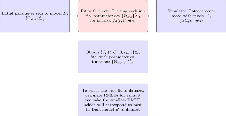
To determine $EDD(B\to A)$, we start by defining $S$ parameter sets ${\Theta }_j$, $j=1,\dots ,S$ for model $A$ for which we determine the incidence curves, that is, we compute the (exact or numerical) solutions for the ODE (1.1) for model $A$ for each parameter set ${\Theta }_j$, and these are our datasets to fit model $B$. We fit model $B$ to each of these curves by using $Q$ different initial parameter sets to execute a numerical program that applies a process of minimization to estimate parameters of model $B$. These initial parameter sets, in turn, are created by using a method of latin hypercube sampling that creates $Q$ random values within a defined range. For instance, for the parameter $K$ we create $Q=10$ values between $0$ and $1000$. Assume now that $y_{t_i}$, $i=1,\dots ,n$, are the points or data for each time $t_i$ of model $A$, and $f(t_i,C;\hat{\Theta })$, are the values of fits obtained with model $B$, where $\hat{\Theta }$ is the set of estimated parameters of model $B$. Then we determine the root mean square error (RMSE)

$$\mathrm{RMSE}≔\sqrt{\frac{1}{n}\sum _{i=1}^n{\left(f(t_i,C;\hat{\Theta })-y_{t_i}\right)}^2}$$

to compute the distance between the data curve, tabulated at $t_1,\dots ,t_n$, and a fit with model $B$ expressed by the values $f(t_i,C;\hat{\Theta })$, $i=1,\dots ,n$. We select the best fit with the smallest RMSE between the $Q$ fits for each of the $S$ data curves (see Fig. 1), and then consider the mean of the $S$ best values of RSME as the distance from model $B$ to model $A$. Besides, we will also calculate the sum of squared errors (SSE) given by

$$\mathrm{SSE}=\sum _{i=1}^n{\left(f(t_i,C;\hat{\Theta })-y_{t_i}\right)}^2,$$

because this quantity naturally arises in the context of least-squares methods. The necessary computations are summarized in Algorithm 2.1 and in Fig. 2.

Fig. 1.

Process to fit the model $B$ to dataset $f_A(t,C;{\Theta }_S)$ generated with model $A$.

Fig. 2.

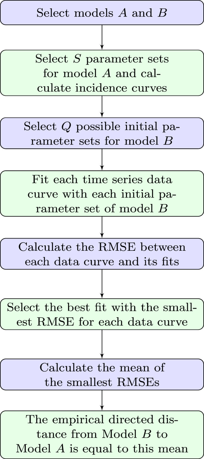
Step by step of measuring the empirical directed distance between two models.

Algorithm 2.1 Calculating $EDD(B\to A)$ —

• Input:

  • –
    Parameter sets ${\left\{{\Theta }_j\right\}}_{j=1,\dots ,S}$ of model $A$ that define the incidence curves

    $${\left\{f_A(t,C;{\Theta }_j)\right\}}_{j=1,\dots ,S},t\in [0,T]$$

    (simulated data).
  • –
    Initial parameter sets ${\left\{{\Theta }_{B,i}\right\}}_{i=1,\dots ,Q}$ of model $B$.
  • –
    Sampling times $t_k$, $k=1,\dots ,n$ at which the incidence curves (both of the simulated data and the approximation) are evaluated.
• for $j=1,\dots ,S$

  • $i^{\ast }\left(j\right)\leftarrow 1$
  • for $i=1,\dots ,Q$

    • (1)
      Determine the vector of estimated parameters ${\hat{\Theta }}_{B,i,j}$ for the $j$th data curve based on the initial parameter vector ${\Theta }_{B,i}$ by Simulated Annealing.
    • (2)
      Calculate

      $${\mathrm{RMSE}}_{ij}=\sqrt{\frac{1}{n}\sum _{k=1}^n{\left(f_B(t_k;C;{\hat{\Theta }}_{B,i,j})-f_A(t_k;C;{\Theta }_j)\right)}^2}.$$
    • (3)
      if ${\mathrm{RMSE}}_{ij}\le {\mathrm{RMSE}}_{i^{\ast }\left(j\right),j}$ then

      • $i^{\ast }\left(j\right)\leftarrow i$
    • endif
  • endfor

• endfor

• Output: the empirical directed distance from model $B$ to model $A$,

  $$EDD(B\to A)\leftarrow \frac{1}{S}\sum _{j=1}^S{\mathrm{RSME}}_{i^{\ast }\left(j\right),j}.$$

2.3. Simulated annealing method for parameter estimation

As we want know the distance between two PGMs, we need numerical methods to calculate the fits from a model $B$ to a model $A$ and in some cases to determine solutions of the ODEs. Then to achieve the best fit it is necessary to estimate parameters, for which we employ the Simulated Annealing method to minimize the Euclidean distance between the curve from model $A$ and the fit with the estimation parameters of model $B$. The Simulated Annealing (SA) method has been useful to solve optimization problems [58], in particular for parameter estimation [52], [59], [60], as in our case, where the goal here is to minimize the function

$$\Theta \mapsto J\left(\Theta \right)≔\sqrt{\sum _{k=1}^n{\left(f(t_k;C;\Theta )-{\mathrm{data}}_{t_k}\right)}^2},$$

being $t\mapsto f(t,C;\Theta )$ the incidence function of a PGM evaluated for a parameter vector $\Theta$ that should satisfy $\Theta \in \mathcal{S}$ for some admissible set $\mathcal{S}$ compatible with the algebraic form of $f$ for $n$ different time points $t_k$, where ${\mathrm{data}}_{t_k}$ correspond to data in time series. In our study, the values ${\left\{{\mathrm{data}}_{t_k}\right\}}_{k=1,\dots ,n}$ are the datasets generated by model $A$, and model $B$ will define the incidence function $f$ and the set $\mathcal{S}$. Hence, the optimization problem at hand can be defined as follows:

$$\text{find }\hat{\Theta }\in \mathcal{S}\text{ such that }J\left(\hat{\Theta }\right)=\underset{\Theta \in \mathcal{S}}{min}J\left(\Theta \right)\text{.}$$ (2.7)

This problem is solved by employing the routines exposed in Appendix.

3. Application of the methodology

3.1. Parameters of specific phenomenological growth models

The methodology of Section 2.2 will allow us to determine the contribution of the scaling parameter $p$ and to observe the closeness between the dynamics of the models $A$ and $B$, where model $A\in \{\mathrm{GLM},\mathrm{RM},\mathrm{GGoM}\}$ is used to generate simulated data or data curves and model $B\in \{\mathrm{LM},\mathrm{GLM},\mathrm{RM},\mathrm{GGoM}\}$, $B\ne A$, is employed to calculate fits. To assess the contribution of the parameter $p$, we select a set of values of $p$ fairly close to $1$ but leave other parameters fixed (taking into account that the parameter $b$ of the GGoM depends on the value of $p$). Then, we analyze the distance of model $B$ to curves generated with model $A$. For example, if we consider $B=\mathrm{LM}$ and its fits to each data curve generated with model $A$, we can calculate the RMSEs, and finally to have the distance from the LM to GLM, RM and GGoM curves. Furthermore, we also calculate the distance from the GLM to RM and GGoM curves, the RM to GLM and GGoM curves and finally from the GGoM m to GLM and RM curves. These processes will be named Experiment 1, 2, 3, and 4, respectively. (All these distances are to be understood in the sense of EDD, of course.)

For the experiments we consider the three parameters $r$, $p$, and $K$. To compare models with equivalent parameters, we choose (as in [16, Sect. 1]) the following expressions for the parameters $b$ and $r$ within the GGoM in terms of the parameter $K$ and the initial value $C\left(0\right)$:

$$r=1-\frac{C\left(0\right)}{K},$$ (3.1)

$$b=\left\{\begin{array}{cc}\frac{r}{log(K∕C\left(0\right))}\hfill & \text{if }p=1\text{,}\hfill \\ \frac{r(1-p)}{K^{1-p}-C{\left(0\right)}^{1-p}}\hfill & \text{if }0<p<1\text{,}\hfill \end{array}\right)$$ (3.2)

where the expression for $p=1$ is the limit of that for $0<p<1$, i.e., 

$$\frac{r}{log(K∕C\left(0\right))}=\underset{p\to 1,p<1}{lim}\frac{r(1-p)}{K^{1-p}-C{\left(0\right)}^{1-p}}.$$

Therefore, to standardize the analysis, we consider the parameter set $\Theta =(r,p,K)$ for all models with $K=1000$, $C\left(0\right)=1$, $r$ determined by (3.1), and $b$ calculated from (3.2) in dependence of the value of the parameter $p$, which is allowed to assume one of the values

$$p\in \mathcal{P}≔\{1,0.995,0.99,0.98,0.95,0.85,0.8\}.$$

Summarizing, we utilize the parameters

$$(r,p,K)=(0.999,p,1000)\text{with }p\in \mathcal{P}\text{.}$$

These values are used directly for the GLM and RM, while for the GGoM we employ the corresponding parameters $(r,p,b)=(0.999,p,b)$ with $b=0.1446$ if $p=1$ and $b=0.1421$, 0.1397, 0.1349, 0.1211, 0.0824, and 0.0670 for $p=0.995$, 0.99, 0.98, 0.95, 0.85, and 0.8, respectively.

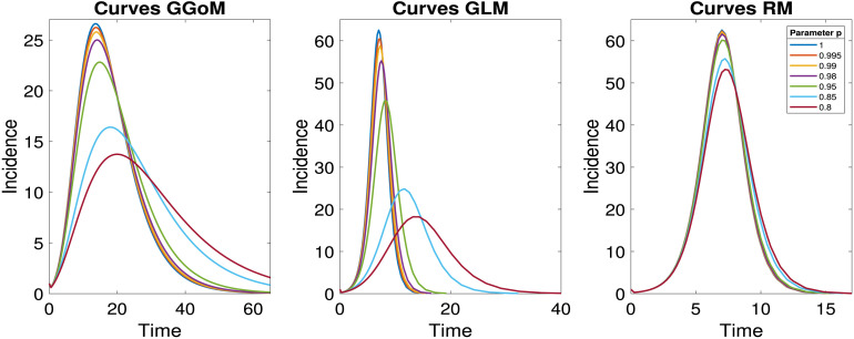
These parameters, listed also in Table 2, produce the data curves shown in Fig. 3. Roughly speaking, these curves illustrate that the role of the parameter $p$ within the GGoM and GLM is to describe the initial growth of the incidence curve, while within the RM the initial phase of the curves, where values of $C\left(t\right)$ are still fairly small, is almost the same for all $p$-values. Furthermore, we see that with decreasing values of $p$ the extremal value (peak) of the incidence curves of the GGoM and GLM decreases rapidly, while that of the RM model decreases only slowly. In addition, the GGoM and GLM exhibit an appreciable shift of the timing of that maximum (i.e., the peak time increases significantly with decreasing $p$) while this effect is not much appreciable for the RM (with the chosen parameters). (For the GGoM and RM the respective closed formulas for $C\left(t\right)$, (2.4), (2.5), may be utilized and differentiated to discuss all these properties in explicit form, see [16].)

Table 2.

Summary of parameters for each model curve .

Parameters for GGoM curves			Parameters for RM curves			Parameters for GLM curves
$r$	$b$	$p$	$r$	$p$	$K$	$r$	$p$	$K$
0.999	0.1446	1.000	0.999	1.000	1000	0.999	1.000	1000
0.999	0.1421	0.995	0.999	0.995	1000	0.999	0.995	1000
0.999	0.1397	0.990	0.999	0.990	1000	0.999	0.990	1000
0.999	0.1349	0.980	0.999	0.980	1000	0.999	0.980	1000
0.999	0.1211	0.950	0.999	0.950	1000	0.999	0.950	1000
0.999	0.0824	0.850	0.999	0.850	1000	0.999	0.850	1000
0.999	0.0670	0.800	0.999	0.800	1000	0.999	0.800	1000

Fig. 3.

Data curves for each growth model.

To help the fits, we generate the data curves from model $A$, with evaluations for every $0<h<1$ time units to have more points or data for fit model $B$ in each case, i.e. we select $t_k=kh$, $k=0,1,2,3,\dots ,n$. For example, we use temporal meshwidth of $h=0.25$ for the GLM curves.

3.2. Application of the simulated annealing (SA) method

The SA method will be used to estimate parameters, as presented in Appendix, where we will use the Matlab function SIMULANNEALBND to implement the SA algorithm. The objective function to minimize is (2.7) for parameter vectors $\Theta$ and functions $f$ that depend on the choice of model $B$ in each case. For simplicity, the application of SA method, we will use the solutions from model B, where by utilizing (2.6), we could recover $f$ in terms of $C$.

For example, the function $f$ within the objective function for $B=\mathrm{LM}$ is calculated by using the solution $C$ to the LM presented in (2.2), i.e. we use the explicit solution of this model, as we also do for the RM with (2.5) and the GGoM with (2.3), (2.4) for the respective cases $p=1$ and $0<p<1$. However, since the GLM does not have a solution in closed algebraic form we employ a numerical approximation to solve the initial value problem to the GLM (see all details in the Appendix).

Then, once the form of the algebraic model under study is given, we need to define the solution spaces for each model which depend on the role of each parameter within each model function. Here the quantities $K$, $C\left(0\right)$, and $p$ are fixed and the expressions for the parameters $r$ and $b$ are given by (3.1), (3.2), respectively. To search the solution spaces for each parameter, we consider the conditions summarized in Table 1 to define the sets specified in Table 3, where we select the initial parameter to run the SA algorithm. This algorithm provides a solution that varies from run to run since the algorithm consists in a random process that utilizes a probability criterion to select the optimal value. However, if we apply the SA algorithm to $Q$ possible initial parameter sets, then with these solutions we can reduce or limit the solution space between the maximum and the minimum best parameters shown for the run. This new solution space helps us to control results and improve the solution and the calculation time. This process follows the idea shown in [52] concerning double-cycle application of SA. The solution spaces that result from the fits for each model $B$ with each data curve are summarized in Table 4.

Table 3.

Initial parameter set for each model B.

Model $B$
LM $\Theta =(r,K)$	GLM $\Theta =(r,p,K)$	RM $\Theta =(r,p,K)$	GGoM $\Theta =(r,b,p)$
$(0,4)\times (0,1000]$	$(0,4)\times (0,1]\times (0,1000]$	$(0,4)\times (0,1]\times (0,1000]$	$(0,4)\times (0,1]\times (0,1]$

Table 4.

Solution spaces for the parameter estimation with each model B and data curves.

Model $B$	Model $A$
	GLM curves	RM curves	GGoM curves
LM $(r,K)$	$[0.5,1.1]\times (700,1010)$	$[0.9,1.1]\times (900,1010)$	$[0.2,0.5]\times [400,800]$
		$[0.8,1]\times [0.2,1]\times [500,1010)$,
		$0.99\le p\le 1$;
GLM $(r,p,K)$		$[0.5,1.5]\times [0.4,0.85]\times [800,1010)$,	$[1.5,1.6]\times [0.5,0.7]\times [800,1000]$
		$0.95\le p<0.99$;
		$[0.5,1]\times [0.4,0.999]\times [900,1010)$,
		$0.8\le p<0.95$
RM $(r,p,K)$	$[0.7,0.99]\times [0.2,0.999]\times [800,1010)$		$[1.8,1.9]\times [0.05,0.08]\times [800,1000],$
			$0.95\le p\le 1$
			$[1.8,2]\times [0.05,0.08]\times [800,1010),$
			$0.8\le p\le 0.25$
GGoM $(r,b,p)$	$(0,3)\times (0,1]\times (0,1]$	$(0,3)\times (0,1]\times (0,1]$

3.3. Experiment 1: empirical directed distances from the logistic model (LM) to other models

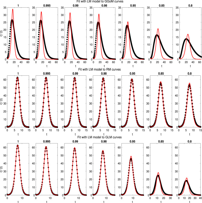
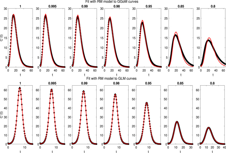
With the best set of initial parameters and the best parameter estimation, we have Fig. 4 with the best fits for the LM, where we can see that the LM is closer to the RM curves, since it captures this dynamics better than for that of the other models. On the other hand, LM is further from GGoM curves, this is due to the long time defined for GGoM data, that the LM exceeds the maximum given by it. A similar situation occurs when the maximum decreases for GLM curves and time increases. The RMSEs calculated to measure the EDD are shown in Table 5 and Fig. 5. It turns out that when the value of $p$ is decreased for the GLM and RM, the error increases more for the GLM than for the RM while a different situation occurs with the GGoM, since the error decreases when $p$ is decreased, but this change is slower than the increase of the error for the GLM and RM. The increase of the RMSE for data generated by the LM is expected because when $p=1$, the dynamics of the LM and that of these models should be the same, where in Table 6 (first row) we can see that the parameter estimation for GLM and RM data curves with $p=1$ are closer to real parameters, i.e., to $\Theta =(r=0.999,p=1,K=1000)$. Another observation about results for parameter estimation summarized in Table 6 is that the growth rate $r$ of the LM for data curves generated by the GGoM is naturally smaller than the growth rate for data generated by the LM, because the GGoM has a slower increase, where for the same reason for GLM data with $p=0.8$ the growth rate decreases to 0.4597.

Fig. 4.

Experiment 1: results of fits of the LM (model $B$) to the curves of data generated by the GGoM (top row), GLM (middle row), and GLM (bottom row), for the indicated values of $p$.

Table 5.

RSME for each data curve, where columns 3 to 9 correspond to the error for the indicated value of $p$, and column 10 shows the mean RMSE, that is, $EDD(B\to A)$.

Model B	Model $A$	Error RMSE to each fit with model $B$							$EDD(B\to A)$
		$p=1$	$p=0.995$	$p=0.99$	$p=0.98$	$p=0.95$	$p=0.85$	$p=0.8$
LM	GGoM	5.2319	5.1864	5.1430	5.1163	5.0480	4.7069	4.4697	5.1163
	GLM	0.1900	0.2455	0.4625	0.8184	1.7021	2.6900	2.6570	0.8184
	RM	0.0568	0.0685	0.0955	0.1706	0.4099	1.1989	1.5615	0.1706
RM	GGoM	0.6827	0.6804	0.7055	0.7668	0.9285	1.3375	1.4244	0.7668
	GLM	0.0037	0.0381	0.0741	0.1347	0.2638	0.3397	0.3066	0.1347
GLM	GGoM	0.4712	0.4757	0.4556	0.4481	0.4284	0.3513	0.3015	0.4481
	RM	0.0069	0.1536	0.0605	0.1993	0.2477	0.7268	1.6235	0.1993
GGoM	GLM	12.1578	11.6221	11.1988	10.2038	7.8028	3.4788	1.8623	10.2038
	RM	12.1667	12.1529	12.0017	12.0359	11.4630	10.1060	9.3656	12.0017

Fig. 5.

Experiment 1: illustrative diagram for the empirical directed distances $EDD(\mathrm{LM}\to \mathrm{GGoM})$, $EDD(\mathrm{LM}\to \mathrm{RM})$, and $EDD(\mathrm{LM}\to \mathrm{GLM})$ based on data curves.

Table 6.

Experiment 1: parameter estimation for LM with GGoM, GLM and RM data curves.

Parameter estimation for LM
CURVES	With GGoM curves		With GLM curves		With RM curves
With $p$	$r$	$K$	$r$	$K$	$r$	$K$
1	0.4193	621.2245	1.0017	1007.1734	1.0012	1001.6787
0.995	0.4149	617.9446	0.9836	997.3534	0.9999	998.2173
0.99	0.4105	617.1784	0.9662	992.6324	0.9989	999.1522
0.98	0.4018	610.0832	0.9310	969.1496	0.9965	996.8109
0.95	0.3756	598.7651	0.8341	941.6386	0.9888	987.6975
0.85	0.2931	554.6741	0.5643	806.5594	0.9600	959.6222
0.8	0.2550	535.9005	0.4597	754.1879	0.9433	946.7694

3.4. Experiment 2: empirical directed distances from the Richards model (RM) to other models

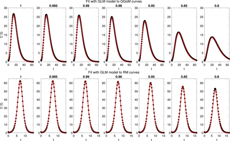
We follow the structure of presentation of results of Experiment 1. In Fig. 6 we can observe that the RM (in the role of model $B$) is closer to the GLM than to the GGoM, where the fits captures almost all the dynamics presented for the GLM data curves. Now with the RMSE calculated, we have effectively the smallest errors for the fit to GLM data, where in Table 5 we see that the RMSE increases faster with GGoM data than with GLM data. Besides, the RMSEs for GLM curves are less than 0.5, evidencing relative closeness between the logistic models. Concerning the parameter estimation (Table 7), we have a good approximation between the parameters for GLM when $p=1$, where the estimated parameter $p$ varies more than the growth rate $r$ to capture the decrease of the maximum value, evidencing a good contribution of this parameter. On the other hand the variation of the parameter $r$ is smaller than that of $p$ and $K$ when the RM is used to fit the GGoM curves.

Fig. 6.

Experiment 2: results of fits of the RM (model $B$) to the curves of data generated by the GGoM (top row) and the GLM (bottom row), for the indicated values of $p$.

Table 7.

Experiment 2: parameter estimation for RM with GGoM and GLM data curves.

Parameter estimation for RM
CURVES	With GGoM curves			With GLM curves
With $p$	$r$	$p$	$K$	$r$	$p$	$K$
1	1.9998	0.0800	954.1139	0.9990	0.9999	1000.0513
0.995	1.9999	0.0798	957.9978	0.9876	0.9732	999.5539
0.99	1.9973	0.0789	953.8977	0.9763	0.9476	999.4866
0.98	1.9912	0.0771	944.5345	0.9547	0.8976	997.8995
0.95	1.9431	0.0740	937.1508	0.9000	0.7532	1000.3445
0.85	1.8952	0.0593	892.6791	0.8000	0.4048	998.1613
0.8	1.9238	0.0500	869.3741	0.8551	0.2612	1003.6135

3.5. Experiment 3: empirical directed distances from the generalized logistic model (GLM) to other models

In Fig. 7, we can see a performance closer to both dynamics with GLM, where this model captures fairly well the maximum value and the length time. Observing the RMSEs 5, we can see that these are smaller than 1.6, as expected when we consider the fits shown in Fig. 7. Now, analyzing Table 5 we observe that the errors increase faster for RM (when $p$ decreases) than with GGoM, where the errors decrease slowly when $p$ decreases. This behavior may be due to the dynamics of the GLM, where if the maximum value decreases, the time length increases, but for the RM data curves, the time length and maximum value are closer to each other. About parameter estimation (see Table 8), we have that for the parameter set with the RM curves the values are closer to parameters of the GLM with $p=1$, i.e, $\Theta =(0.999,1,1000)$. This, because, the RM curves vary little of the RM initial curve with $p=1$. The previous result contrasts with the fit for GGoM curves, because when the parameter $p$ varies for GGoM curves, the maximum value decreases and the time length increases, where with the GGoM the length time is the same when the parameter $p$ decreases. For this reason the parameter estimation for the GGoM curves varies the parameter $p$ more than others.

Fig. 7.

Experiment 3: results of fits of the GLM (model $B$) to the curves of data generated by the GGoM (top row) and the RM (bottom row), for the indicated values of $p$.

Table 8.

Experiment 3: parameter estimation for GLM with GGoM and RM data curves.

Parameter estimation for GLM
CURVES	With GGoM curves			With RM curves
With $p$	$r$	$p$	$K$	$r$	$p$	$K$
1	1.5402	0.6744	998.0430	0.9994	0.9999	1000.1965
0.995	1.5293	0.6734	986.8504	1.0000	0.9999	999.3734
0.99	1.5054	0.6743	989.5241	1.0000	0.9991	1000.4114
0.98	1.5221	0.6670	992.3809	1.0000	0.9984	1003.5106
0.95	1.5278	0.6508	992.7939	1.0000	0.9961	992.1099
0.85	1.5204	0.5962	994.5254	1.0000	0.9876	971.7100
0.8	1.5112	0.5678	989.0751	0.9888	0.9850	915.3278

Table 9.

Experiment 4: parameter estimation for GGoM with GLM and RM data curves.

Parameter estimation for GGoM
CURVES	With GLM curves			With RM curves
With $p$	$r$	$b$	$p$	$r$	$b$	$p$
1	2.3207	0.3237	1.0000	2.3516	0.3279	1.0000
0.995	2.3068	0.3220	1.0000	2.2635	0.3159	1.0000
0.99	2.2932	0.3201	1.0000	2.2761	0.3178	1.0000
0.98	2.1953	0.3068	1.0000	2.4303	0.3326	0.9948
0.95	1.9338	0.2712	1.0000	2.2822	0.3187	1.0000
0.85	1.2596	0.1678	0.9823	2.2986	0.3214	1.0000
0.8	1.2670	0.1500	0.9496	2.2716	0.3180	1.0000

3.6. Experiment 4: empirical directed distances from the generalized Gompertz model (GGoM) to other models

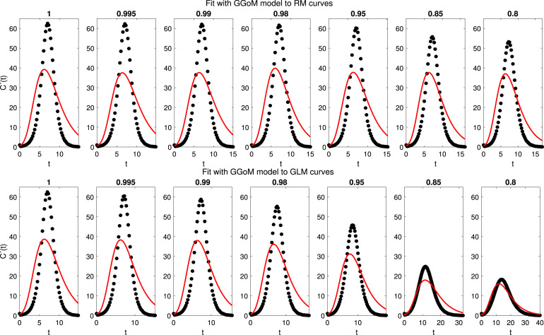
For this experiment, we consider the GGoM model as model $B$, and the models $A$ are RM and GLM, with the parameters summarized in Table 2. In Fig. 8 we can see the fits for RM and GLM data curves. This figure indicates that the GGoM does not capture the dynamics of the logistic models, where the maximum values are very large for the period of time defined in these data curves. The RMSEs in Table 5 are very large if compared with the previous experiments. The errors decrease when the parameter $p$ is decreased, but this situation is due to approximation between the maximum values of the data curves and the maximum value that the GGoM can reach with the given period of time.

Fig. 8.

Experiment 4: results of fits of the GGoM (model $B$) to the curves of data generated by the RM (top row) and the GLM (bottom row), for the indicated values of $p$.

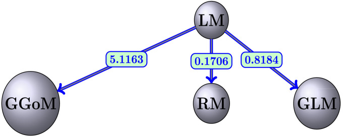
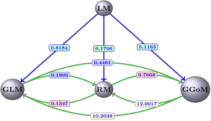
Finally, the parameter estimation obtained for each fit is summarized in Table 9, where we observe that the parameter $p$ is almost fixed. Being for the RM curves the other parameters almost equally fixed, this is due to the slow decrease for the maximum value. This contrasts with the result for the GLM, where the maximum value decreases faster than for the RM. For this reason the parameters $r$ and $b$ are varying. Summarizing, we have in Fig. 9 the distances presented among the models studied, where each arrow indicates the direction of the distance from model $B$ to model $A$.

Fig. 9.

Comparative graph for each EDD and model.

4. Examples: Application to real data

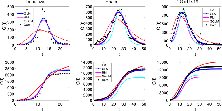
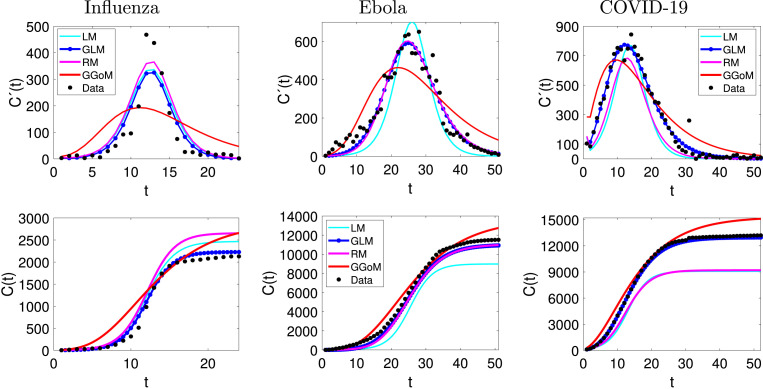
In order to see the best performance evidenced by the GLM model when capturing the other dynamics studied in the experiments performed, we present three examples with real data. In this case, we consider the data of weekly cases of influenza in Chile (24 data points in total) produced between autumn and winter of 2009 [61], Ebola (51 data points in total) in Sierra Leone dating from 2014 [62] and recent outbreak of COVID-19 [63] presented in various provinces of China (excluding Hubei province) (52 data points in total). Since we consider real data, for the application of the procedure of Section 3 we replace model $A$ by real data but keep employing the same methodology of Section 3 with model $B$, where we also create a refinement of the real data by interpolation from the cumulative curve $C$, achieving for these examples twice the original number of points. From the RMSEs calculated and registered in Table 10 and the bar chart of Fig. 10 we observe that the RMSEs for the non-interpolated data are close to the double from the RMSEs for the interpolated data, where effectively GLM meets be the best model with the smaller RMSE to the three examples.

Table 10.

Application to real data: RSME for different time refinements.

Model	Influenza		Ebola		COVID-19
	Interpolation	No interpolation	Interpolation	No interpolation	Interpolation	No interpolation
LM	28.4864	55.5662	44.5472	90.0674	59.6479	108.9944
GLM	26.2694	49.7601	24.4430	47.8958	21.2940	45.4623
GGoM	52.7972	113.9227	51.8345	94.6347	174.9620	356.6672
RM	29.1628	55.8399	26.2160	53.3493	54.9620	109.9705

Fig. 10.

Application to real data: bar charts for the RMSE for each real data and refinement time.

From the figures of the fits, with and without interpolation (see Fig. 11, Fig. 12) for three examples, we can observe that the refinement from real data does not have a great impact on the performance of the GGoM (red), but in the Ebola case this model for early growth produces a better fit than others. For the fits made with the LM, we can observe that for the case of influenza the refinement leaves the fit similar to a fit without interpolation where for this case, the LM is better than the RM. A different situation occurs for the Ebola and COVID-19 cases where for Ebola the maximum value for the incidence curve increases and the cumulative curve increases close to real cumulative curve, though this is not better than the fits by the GLM and the RM. For COVID-19 the LM decreases the maximum value for the incidence curve and the cumulative curve decreases close to the cumulative curve of the RM, although this is not better than the fits by the GLM and RM. Now if we observe the fits with the RM and the GLM, we see that their fits though very similar for Ebola data, the GLM fits are better where the RMSE is smaller. On the other hand, with influenza data, we can see that for RM and GLM models, the curve with GLM is above the RM curve, staying in the middle the LM curve, and the situation changes when the data are interpolated, where the RM curve turns out to be above the GLM and LM curves, but the GLM produces the best fit with the smallest RMSE. In the case of COVID-19, the fits with the GLM with and without interpolated data are very close. A different situation occurs with the RM where the fits to the interpolated and non-interpolated data are below the data and therefore with RMSEs bigger than those for the GLM. Furthermore, Table 11 indicates that for the parameter estimation the values are very close between the real data and interpolated data, where for the LM this shows smaller variations and the GGoM model shows more variations with Ebola data.

Fig. 11.

Application to raw data: fits to influenza, Ebola and COVID-19 data.

Fig. 12.

Application to interpolated data: fits to influenza, Ebola and COVID-19 data.

Table 11.

Application to real data: Parameter estimation for fit with real data.

Model	Influenza	Ebola	COVID-19
Interpolation
LM	$(0.5561,2467.9)$	$(0.3141,8988.2)$	$(0.3413,9074.6586)$
GLM	$(0.5964,1,2228.8)$	$(0.7481,0.8546,10989)$	$(3.6232,0.6869,12963.9057)$
GGoM	$(1.244,0.1809,1)$	$(1.0000,0.0897,0.9487)$	$(5.7818,0.0989,0.6709)$
RM	$(0.5603,1,2655.7)$	$(0.4189,0.4273,11057)$	$(0.4188,0.6302,9196.4353)$
No interpolation
LM	$(0.5565,2475.9)$	$(0.3127,8327.7)$	$(0.3426,9844.7509)$
GLM	$(0.6003,1,2363.1)$	$(0.7640,0.8515,11212)$	$(2.7782,0.7213,12316.4258)$
GGoM	$(1.2434,0.1800,1)$	$(0.8134,0.0968,1.0000)$	$(5.0086,0.1020,0.6931)$
RM	$(0.55451,2392.5)$	$(0.4326,0.4000,11698)$	$(0.4133,0.6472,9145.3252)$

5. Conclusions

First of all, let us recall that the purpose of this work is not primarily a fit of determined phenomenological growth models to specific data but to introduce a general methodology of applying statistics to medicine and biology. Nevertheless, we may briefly comment the specific outcome for the five models studied in this paper before coming to possible extensions.

Overall, we can say that in light of the results of the application of the methodology to different types of growth curves, the GLM produces curves that are closer to the (simulated) data than other models, and the curves produced by the GGoM are most distant to the other models. Besides, the results indicate that introducing the parameter $p$ within the GLM and RM significantly improves the adjustment compared with the original logistic model (LM), while most results obtained with the GGoM lead to parameters $p\approx 1$ in most fits, that is, the GGoM is essentially reduced to the GoM with parameters $\Theta =(r,b)$ with $p=1$. To further highlight the value of the GLM, we mention that this model does not only better approximate the dynamics of data obtained by simulation with other models but as Section 4 illustrates, also captures better real data due the advantageous contribution of the growth scaling parameter $p$. This fact is also demonstrated in our previous work [16]. A possible “mechanistic” explanation of the superiority of the GLM could be related to the different degrees of influence of the parameters. For example, within the GLM we have $C\left(t\right)\to K$ as $t\to \infty$, so we simply need to adjust $K$ to specify a final size of the epidemic while varying $r$ and $p$ does not affect this property. In contrast, as follows from (2.4) (see also [16]), for the GGoM with $0<p<1$ we have

$$C\left(t\right)\to {\left((1-p)(r∕b)+C{\left(0\right)}^{1-p}\right)}^{1∕(1-p)}\text{as }t\to \infty \text{,}$$

which means that the final size of the epidemic depends on a number of parameters, in particular the exponent $p$ that is supposed to characterize early growth, and on the initial size of the epidemic $C\left(0\right)$, which is usually a small number that can hardly be determined with certainty. Probably the fact that within the GLM the early and late stages of the epidemic are dominantly influenced by different parameters, namely $p$ and $r$; and $K$, respectively, provides an advantage for reliable parameter identification.

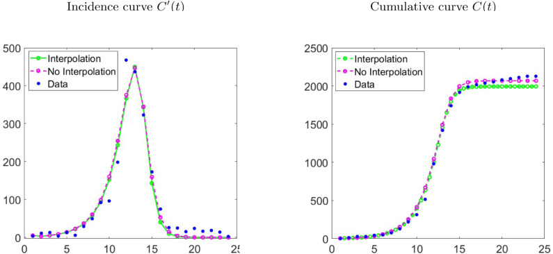
Our interest in the range $0<p<1$ for the GLM and GGoM comes from the wish to characterize sub-exponential initial growth, as is motivated in [54], [55], [56]. However, this same parameter $p$ can have another nature in the RM, where there are studies with $p>1$, for example, the papers [64], [65], where we recall that in [16] it was stated that the parameter $p$ within the RM does not serve as an adjustable parameter to capture sub-exponential initial growth. Rather, by its position within the RM the parameter $p$ could allow the shape of upper part of the cumulative curve to be independent of the shape of the lower part, i.e., measures the extent of deviation from the S-shaped dynamics of the classical logistic growth model. Besides, as the parameter $p$ tends to zero, the RM curve tends towards the Gompertz growth curve in the sense $\mathrm{d}C∕\mathrm{d}t=rC\left(t\right)ln(K∕C\left(t\right))$ (see our discussion of the autonomous form of the Gompertz differential equation in Section 2.1). There are other studies on different forms to generalize PGMs, as [64] which shows for case of logistic growth, different to our idea of generalized growth model with $rC{\left(t\right)}^p$, where $p$ is a scaling parameter. Therefore future work will study the EDDs distances between other generalized PGMs. Then if we consider the range $p>1$ for the RM, we can see that this model captures the dynamics of influenza data better than the GLM, as is evidenced in Fig. 13 and Table 12.

Fig. 13.

Application to real data: fits with Richards Model ($p>1$) for influenza data.

Table 12.

Application to real data: Results for different time refinements and real data for RM model with $p>1$.

Results	Influenza	Ebola	COVID-19
Interpolation
RMSE	17.2332	26.2223	46,9405
Parameter
Estimation	$(0.4883,3,1993.2)$	$(0.4173,0.4308,11036)$	$(0.4551,0.5408,9895.1873)$
No interpolation
RMSE	28.7735	51.6678	100,3531
Parameter
Estimation	$(0.49,2.6641,2068.1)$	$(0.4228,0.4191,11182)$	$(0.4350,0.5877,9556.1028)$

We emphasize that our restriction to just five PGMs (namely the LM, GLM, GoM, GGoM, and RM) does in no way represent a limitation inherent to the present approach. In fact, it is not the intention of the present work to provide an exhaustive survey of PGMs in epidemiology but to introduce a methodology to compare PGMs within a small selection with each other. In this sense, other models could be examined as well with the same methodology. For instance, one could consider the four-parameter so-called generalized Richards model (GRM; see [1], [21], [23]) given by

$$f(t,C;\Theta )=r{C}^p\left(1-{(C∕K)}^q\right),\Theta =(r,p,q,K),r,q,K>0,0<p\le 1$$

that combines the generalizations of the GLM (1.2) and the RM (1.5).

Finally, we remark that the methodology of the present work could also be applied to other applications where describing growth by phenomenological models is of interest. As an example, we mentioned in Section 1.2 the growth of tumors. In fact, there is a wealth of alternative phenomenological growth models designed for that application, and to which the present methodology could be applied in future work. We refer to [36], [38], [48] for overviews, and as one specific example the so-called Gomp-ex law (proposed in [45]; see [36]) that for the autonomous form (2.1) can be specified as

$$\phi (C;\Theta )=(t,C;\Theta )=\left\{\begin{array}{cc}C(a-bln{C}_{\mathrm{crit}})\hfill & \text{if }0<C<C_{\mathrm{crit}}\text{,}\hfill \\ C(a-blnC)\hfill & \text{if }C\ge C_{\mathrm{crit}}\text{,}\hfill \end{array}\right)\Theta =(a,b,C_{\mathrm{crit}}),$$

where the Gompertz law (under suitable choices of the constants $a$ and $b$) comes into effect only for sufficiently large populations (i.e., whose size is larger or equal to a given critical size $C_{\mathrm{crit}}$), but below $C_{\mathrm{crit}}$ growth is exponential [36].

Declaration of Competing Interest

The authors declare that they have no known competing financial interests or personal relationships that could have appeared to influence the work reported in this paper.

Appendix. MATLAB Programs

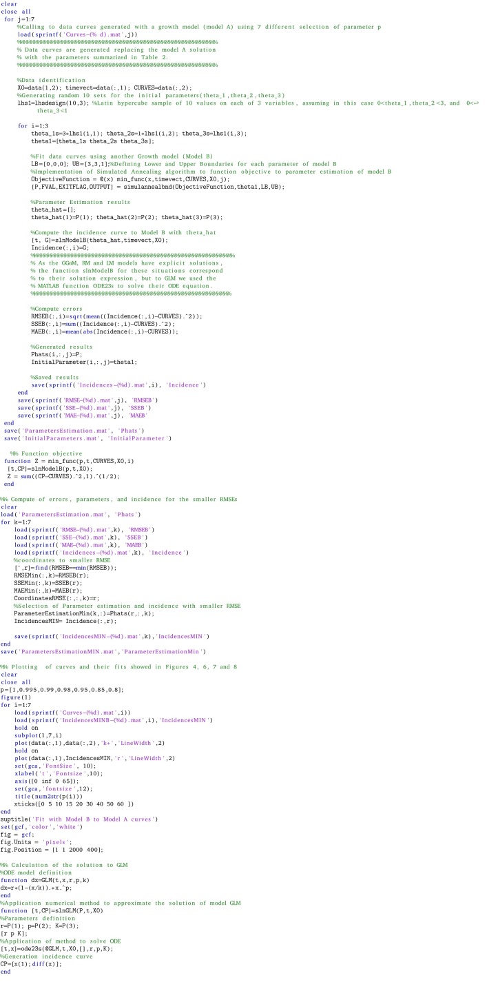
Several numerical calculations contained in this work have been performed by using MATLAB routines, in particular, to implement Simulated Annealing we used different MATLAB functions, such as SIMULANNEALBND, LHSDESIGN, and ODE23S. In the following we expose the codes used to compute the parameter estimation, errors, and the plots presented in Section 3.2.

References

- 1.Chowell G. Fitting dynamic models to epidemic outbreaks with quantified uncertainty: A primer for parameter uncertainty, identifiability, and forecast. Infect. Disease Model. 2017;2:379–398. doi: 10.1016/j.idm.2017.08.001. [DOI] [PMC free article] [PubMed] [Google Scholar]
- 2.Verhulst P.-F. Notice sur la loi que la population suit dans son accroissement. Corresp. Math. Phys. 1838;10:113–121. [Google Scholar]
- 3.Gompertz B. On the nature of the function expressive of the law of human mortality, and on a new mode of determining the value of life contingencies. Phil. Trans. R. Soc. Lond. 1825;115:513–583. doi: 10.1098/rstb.2014.0379. [DOI] [PMC free article] [PubMed] [Google Scholar]
- 4.Richards F.J. A flexible growth function for empirical use. J. Exp. Bot. 1959;10:290–301. [Google Scholar]
- 5.Wang X.S., Wu J., Yang Y. Richards model revisited: Validation by and application to infection dynamics. J. Theoret. Biol. 2012;313:12–19. doi: 10.1016/j.jtbi.2012.07.024. [DOI] [PubMed] [Google Scholar]
- 6.Murray J.D. Springer-Verlag; New York: 2002. Mathematical Biology: I. an Introduction. [Google Scholar]
- 7.Jones D.S., Sleeman B.D. Chapman & Hall/CRC; Boca Raton, FL: 2003. Differential Equations and Mathematical Biology. [Google Scholar]
- 8.Britton N.F. Springer-Verlag; London: 2003. Essential Mathematical Biology. [Google Scholar]
- 9.Brauer F., Castillo-Chavez C. Second Ed. Springer; New York: 2012. Mathematical Models in Population Biology and Epidemiology. [Google Scholar]
- 10.Diekmann O., Heesterbeek J., Britton T. Princeton University Press; 2012. Mathematical Tools for UnderstandIng Infectious Disease Dynamics, Princeton Series in Theoretical and Computational Biology. [Google Scholar]
- 11.Segel L.A., Edelstein-Keshet L. SIAM; Philadelphia, PA: 2013. A Primer on Mathematical Models in Biology. [Google Scholar]
- 12.Turner Jr M.E., Bradley Jr E.L., Kirk K.M., Pruitt K.A. A theory of growth. Math. Biosci. 1976;29:367–373. [Google Scholar]
- 13.Brauer F., Kribs C. CRC Press; Boca Raton, FL, USA: 2016. Dynamical Systems for Biological Modeling: An Introduction. [Google Scholar]
- 14.Anderson R.M., May R.M. Oxford University Press; 1991. Infectious Diseases of Humans, Dynamics and Control. [Google Scholar]
- 15.Yan P., Chowell G. Springer Nature; Cham, Switzerland: 2019. Quantitative Methods for Investigating Infectious Disease Outbreaks. [Google Scholar]
- 16.Bürger R., Chowell G., Lara-Díaz L.Y. Comparative analysis of phenomenological growth models applied to epidemic outbreaks. Math. Biosci. Eng. 2019;16:4250–4273. doi: 10.3934/mbe.2019212. [DOI] [PubMed] [Google Scholar]
- 17.Chowell G., Nishiura H., Bettencourt L.M.A. Comparative estimation of the reproduction number for pandemic influenza from daily case notification data. J. R. Soc. Interface. 2007;4:155–166. doi: 10.1098/rsif.2006.0161. [DOI] [PMC free article] [PubMed] [Google Scholar]
- 18.Arenas A.R., Thackar N.B., Haskell E.C. The logistic growth model as an approximating model for viral load measurements of influenza A virus. Math. Comput. Simulation. 2017;133:206–222. [Google Scholar]
- 19.Chowell G., Viboud C., Hyman J.M., Simonsen L. The Western Africa Ebola virus disease epidemic exhibits both global exponential and local polynomial growth rates. PLOS Curr. Outbreaks. 2015;7 doi: 10.1371/currents.outbreaks.8b55f4bad99ac5c5db3663e916803261. [DOI] [PMC free article] [PubMed] [Google Scholar]
- 20.Chowell G., Viboud C., Simonsen L., Merler S., Vespignani A. Perspectives on model forecasts of the 2014–2015 Ebola epidemic in West Africa: lessons and the way forward. BMC Med. 2017;15:8. doi: 10.1186/s12916-017-0811-y. article 42. [DOI] [PMC free article] [PubMed] [Google Scholar]
- 21.Pell B., Kuang Y., Viboud C., Chowell G. Using phenomenological models for forecasting the 2015 Ebola challenge. Epidemics. 2018;22:62–70. doi: 10.1016/j.epidem.2016.11.002. [DOI] [PubMed] [Google Scholar]
- 22.Viboud C., Sun K., Gaffey R., Ajelli M., Fumanelli L., Merler S., Zhang Q., Chowell G., Simonsen L., Vespignani A. The RAPIDD ebola forecasting challenge: Synthesis and lessons learnt. Epidemics. 2018;22:13–21. doi: 10.1016/j.epidem.2017.08.002. [DOI] [PMC free article] [PubMed] [Google Scholar]
- 23.Chowell G., Hincapie-Palacio D., Ospina J., Pell B., Tariq A., Dahal S., Moghadas S., Smirnova A., Simonsen L., Viboud C. Using phenomenological models to characterize transmissibility and forecast patterns and final burden of Zika epidemics. PLoS Curr. Outbreaks. 2016 doi: 10.1371/currents.outbreak.f14b2217c902f453d9320a43a35b9583. [DOI] [PMC free article] [PubMed] [Google Scholar]
- 24.Brown M., Cain C., Whitfield J., Ding E., Del Valle S.Y., Manore C.A. Preprint BioRxiv 365155. 2018. Modeling Zika virus spread in Colombia using google search queries and logistic power models. [DOI] [Google Scholar]
- 25.Zhao S., Musa S.S., Fu H., He D., Qin J. Simple framework for real-time forecast in a data-limited situation: the Zika virus (ZIKV) outbreaks in Brazil from 2015 to 2016 as an example. Parasites Vectors. 2019;12:13. doi: 10.1186/s13071-019-3602-9. article 344. [DOI] [PMC free article] [PubMed] [Google Scholar]
- 26.Del Valle S.Y., McMahon B.H., Asher J., Hatchett R., Lega J.C., Brown H.E., Leany M.E., Pantazis Y., Roberts D.J., Moore S., Peterson A.T., Escobar L.E., Qiao H., Hengartner N.W., Mukundan H. Summary results of the 2014-2015 DARPA chikungunya challenge. BMC Infect. Diseases. 2018;18:9. doi: 10.1186/s12879-018-3124-7. article 245. [DOI] [PMC free article] [PubMed] [Google Scholar]
- 27.Mizumoto K., Kagaya K., Chowell G. Early epidemiological assessment of the transmission potential and virulence of Coronavirus disease 2019 (COVID-19) in Wuhan City, China, january-february, 2020. BMC Med. 2020;18:9. doi: 10.1186/s12916-020-01691-x. article 217. [DOI] [PMC free article] [PubMed] [Google Scholar]
- 28.Roosa K., Lee Y., Luo R., Kirpich A., Rothenberg R., Hyman J.M., Yan P., Chowell G. Real-time forecasts of the COVID-19 epidemic in China from february 5th to february 24th, 2020. Infect. Disease Model. 2020;5:256–263. doi: 10.1016/j.idm.2020.02.002. [DOI] [PMC free article] [PubMed] [Google Scholar]
- 29.Faranda D., Pérez Castillo I., Hulme O., Jezequel A., Lamb J.S.W., Sato Y., Thompson E.L. Asymptomatic estimates of SARS-CoV-2 infection counts and their sensitivity to stochastic perturbation. Chaos. 2020;30:10. doi: 10.1063/5.0008834. 051107. [DOI] [PMC free article] [PubMed] [Google Scholar]
- 30.Catala M., Alonso S., Alvarez-Lacalle E., Lopez D., Cardona P.J., Prats C. Empiric model for short-time prediction of COVID-19 spreading. PLoS Comput. Biol. 2020;16:18. doi: 10.1371/journal.pcbi.1008431. 1008431. [DOI] [PMC free article] [PubMed] [Google Scholar]
- 31.Consolini G., Materassi M. A stretched logistic equation for pandemic spreading. Chaos Solitons Fractals. 2020;140:9. doi: 10.1016/j.chaos.2020.110113. 110113. [DOI] [PMC free article] [PubMed] [Google Scholar]
- 32.Vasconcelos G.L., Macêdo A.M.S., Duarte-Filho G.C., Araújo A.A., Ospina R., Almeida F.A.G. Preprint (2020), MedRxiv. 2020. Complexity signatures in the COVID-19 epidemic: power law behaviour in the saturation regime of fatality curves; p. 16. [DOI] [Google Scholar]
- 33.Vasconcelos G.L., Macêdo A.M.S., Ospina R., Almeida F.A.G., Duarte-Filho G.C., Brum A.A., Souza I.C.L. Modelling fatality curves of COVID-19 and the effectiveness of intervention strategies. PeerJ. 2020;8:16. doi: 10.7717/peerj.9421. article 9421. [DOI] [PMC free article] [PubMed] [Google Scholar]
- 34.Ohnishi A., Namekawa Y., Fukui T. Universality in COVID-19 spread in view of the Gompertz function. Progr. Theoret. Exper. Phys. 2020;2020:20. 123J01. [Google Scholar]
- 35.Chowell G. Fitting dynamic models to epidemic outbreaks with quantified uncertainty: A primer for parameter uncertainty, identifiability, and forecast. Infect. Disease Model. 2017;2:379–398. doi: 10.1016/j.idm.2017.08.001. [DOI] [PMC free article] [PubMed] [Google Scholar]
- 36.d’Onofrio A., Fasano A., Monechi B. A generalization of Gompertz law compatible with the Gyllenberg-Webb theory for tumour growth. Math. Biosci. 2011;230:45–54. doi: 10.1016/j.mbs.2011.01.001. [DOI] [PubMed] [Google Scholar]
- 37.Ledzewicz U., Olumoye O., Schättler H. On optimal chemotherapy with a strongly targeted agent for a model of tumour-immune system interactions with generalized logistic growth. Math. Biosci. Eng. 2013;10:787–802. doi: 10.3934/mbe.2013.10.787. [DOI] [PubMed] [Google Scholar]
- 38.Talkington A., Durrett R. Estimating tumor growth rates in vivo. Bull. Math. Biol. 2015;77:1934–1954. doi: 10.1007/s11538-015-0110-8. [DOI] [PMC free article] [PubMed] [Google Scholar]
- 39.Vynnycky E., White R.G. Oxford University Press; 2010. An Introduction To Infectious Disease Modelling. [Google Scholar]
- 40.Todeschini R., Consonni V., Pavan M. A distance measure between models: a tool for similarity/diversity of model populations. Chemometr. Intellig. Laborat. Syst. 2004;70:55–61. [Google Scholar]
- 41.Chowell G., Viboud C., Simonsen L., Moghadas S.M. Characterizing the reproduction number for epidemics with sub-exponential growth dynamics. J. R. Soc. Interface. 2016;13:12. doi: 10.1098/rsif.2016.0659. 20160659. [DOI] [PMC free article] [PubMed] [Google Scholar]
- 42.L. Edelstein-Keshet, Mathematical Models in Biology, Random House, New York, 1988.
- 43.Braun M. Fourth Ed. Springer-Verlag; New York: 1993. Differential Equations and their Applications. [Google Scholar]
- 44.Strogatz S.H. Perseus Books; Reading, MA: 1994. Nonlinear Dynamics and Chaos. [Google Scholar]
- 45.Wheldon T.E. Hilger; Bristol and Philadelphia: 1988. Mathematical Models in Cancer Research. [Google Scholar]
- 46.Aroesty J., Lincoln T., Shapiro N., Boccia G. Tumor growth and chemotherapy: mathematical methods, computer simulations, and experimental foundations. Math. Biosci. 1973;17:243–300. [Google Scholar]
- 47.Newton C.M. Biomathematics in oncology: modeling of celular systems. Ann. Rev. Biosci. Bioeng. 1980;9:541–579. doi: 10.1146/annurev.bb.09.060180.002545. [DOI] [PubMed] [Google Scholar]
- 48.de Vladar H.P. Density-dependence as a size-independent regulatory mechanism. J. Theoret. Biol. 2006;238:245–256. doi: 10.1016/j.jtbi.2005.05.014. [DOI] [PubMed] [Google Scholar]
- 49.d’Onofrio A. Fractal growth of tumors and other cellular populations: Linking the mechanistic to the phenomenological modeling and vice versa. Chaos Solitons Fractals. 2009;41:875–880. [Google Scholar]
- 50.Vidal R.V.V. Applied Simulated Annealing. Springer-Verlag; Berlin, Germany: 1993. (Lecture Notes in Economics and Mathematical System). [Google Scholar]
- 51.Buonomo B., Manfredi P., d’Onofrio A. Optimal time-profiles of public health intervention to shape voluntary vaccination for childhood diseases. J. Math. Biol. 2019;78:1089–1113. doi: 10.1007/s00285-018-1303-1. [DOI] [PubMed] [Google Scholar]
- 52.Román-Román P., Romero D., Rubio M.A., Torres-Ruiz F. Estimating the parameters of a Gompertz-type diffusion process by means of simulated annealing. Appl. Math. Comput. 2012;218 5131–5131. [Google Scholar]
- 53.Kühleitner M., Brunner N., Nowak W.-G., Renner-Martin K., Scheicher K. Best-fitting growth model curves of the Bertalanffy-Pütter type. Poultry Sci. 2019;98:3587–3592. doi: 10.3382/ps/pez122. [DOI] [PMC free article] [PubMed] [Google Scholar]
- 54.Viboud C., Simonsen L., Chowell G. A generalized-growth model to characterize the early ascending phase of infectious disease outbreaks. Epidemics. 2016;15:27–37. doi: 10.1016/j.epidem.2016.01.002. [DOI] [PMC free article] [PubMed] [Google Scholar]
- 55.Chowell G., Viboud C. Is it growing exponentially fast?—Impact of assuming exponential growth for characterizing and forecasting epidemics with initial near-exponential growth dynamics. Infect. Disease Model. 2016;1:71–78. doi: 10.1016/j.idm.2016.07.004. [DOI] [PMC free article] [PubMed] [Google Scholar]
- 56.Chowell G., Sattenspiel L., Bansal S., Viboud C. Mathematical models to characterize early epidemic growth: A review. Phys. Life Rev. 2016;18:66–97. doi: 10.1016/j.plrev.2016.07.005. [DOI] [PMC free article] [PubMed] [Google Scholar]
- 57.Ohnishi S., Yamakawa T., Akamine T. On the analytical solution of the Pütter-Bertalanffy growth equation. J. Theoret. Biol. 2014;343:174–177. doi: 10.1016/j.jtbi.2013.10.017. [DOI] [PubMed] [Google Scholar]
- 58.Brooks S.P., Morgan B.J.T. Optimization using simulated annealing. J. Roy. Stat. Soc. Ser. D (The Statistician) 1995;44:241–257. [Google Scholar]
- 59.Abbasi B., Jahromi A.H.E., Arkat J., Hosseinkouchack M. Estimating the parameters of Weibull distribution using simulated annealing algorithm. Appl. Math. Comput. 2006;183:85–93. [Google Scholar]
- 60.Chuine I., Cour P., Rousseau D.D. Fitting models predicting dates of flowering of temperate-zone trees using simulated annealing. Plant, Cell Environ. 1998;21:455–466. [Google Scholar]
- 61.Ministerio de Salud Chile . 2009. Influenza Pandemia (H1N1) Circular de Vigilancia epidemiología de influenza. Available from: http://epi.minsalud.cl/epi/html/normas/circul/CircularInfluenzaESTACIONALyPANDEMICA.pdf. [Google Scholar]
- 62.2015 Ebola response roadmap—Situation report—14 2015, in: See http://apps.who.int/ebola/current-situation/ebola-situation-report-14-october-2015 (accessed 17 2015).
- 63.Chinese National Health Committee, in: Reported cases of 2019-nCoV, Retrieved from https://ncov.dxy.cn/ncovh5/view/pneumonia?from=groupmessage&isappinstalled=0.
- 64.Tsoularis A., Wallace J. Analysis of logistic growth models. Math. Biosci. 2002;179:21–55. doi: 10.1016/s0025-5564(02)00096-2. [DOI] [PubMed] [Google Scholar]
- 65.Birch C. A new generalized logistic sigmoid growth equation compared with the Richards growth equation. Ann. Botany. 1999;83:713–723. [Google Scholar]