

Abstract
Motivation
Protein function prediction is a difficult bioinformatics problem. Many recent methods use deep neural networks to learn complex sequence representations and predict function from these. Deep supervised models require a lot of labeled training data which are not available for this task. However, a very large amount of protein sequences without functional labels is available.
Results
We applied an existing deep sequence model that had been pretrained in an unsupervised setting on the supervised task of protein molecular function prediction. We found that this complex feature representation is effective for this task, outperforming hand-crafted features such as one-hot encoding of amino acids, k-mer counts, secondary structure and backbone angles. Also, it partly negates the need for complex prediction models, as a two-layer perceptron was enough to achieve competitive performance in the third Critical Assessment of Functional Annotation benchmark. We also show that combining this sequence representation with protein 3D structure information does not lead to performance improvement, hinting that 3D structure is also potentially learned during the unsupervised pretraining.
Availability and implementation
Implementations of all used models can be found at https://github.com/stamakro/GCN-for-Structure-and-Function.
Supplementary information
Supplementary data are available at Bioinformatics online.
1 Introduction
Proteins perform most of the functions necessary for life. However, proteins with a well-characterized function are only a small fraction of all known proteins and mostly restricted to a few model species. Therefore, the ability to accurately predict protein function has the potential to accelerate research in fields such as animal and plant breeding, biotechnology and human health.
The most common data type used for automated function prediction (AFP) is the amino acid sequence, as conserved sequence implies conserved function (Kimura and Ohta, 1974). Consequently, many widely used AFP algorithms rely on sequence similarity via BLAST (Altschul et al., 1990) and its variants or on hidden Markov models (Eddy, 2009). Other types of sequence information that have been used include k-mer counts, predicted secondary structure, sequence motifs, conjoint triad features and pseudo-amino acid composition (Cozzetto et al., 2016; Fa et al., 2018; Sureyya Rifaioglu et al., 2019). Moreover, Cozzetto et al. showed that different sequence features are informative for different functions.
More recently, advances in machine learning have partially shifted the focus from hand-crafted features, such as those described above, to automatic representation learning, where a complex model—most often a neural network—is used to learn features that are useful for the prediction task at hand. Many such neural network methods have been proposed, which use a variety of architectures (Bonetta and Valentino, 2020).
Some studies combined the two approaches, starting from hand-crafted features that are fed into a multi-layer perceptron (MLP) to learn more elaborate representations (Fa et al., 2018; Sureyya Rifaioglu et al., 2019). Others apply recurrent or convolutional architectures to directly process variable-length sequences. For instance, Kulmanov et al. (2018) used a neural embedding layer to embed all possible amino acid triplets into a 128-dimensional space and then applied a convolutional neural network (CNN) on these triplet embeddings. Moreover, Liu (2017) and Cao et al. (2017) trained Long Short-Term Memory (LSTM) networks to perform AFP.
The motivation behind these deep models is that functional information is encoded in the sequence in a complicated way. A disadvantage is that complex models with a large number of parameters require a large amount of training examples, which are not available for the AFP task. There are about 80 000 proteins with at least one experimentally derived Molecular Function Gene Ontology (GO) (Ashburner et al., 2000) annotation in SwissProt and 11 123 terms in total.
In contrast, a huge number of protein sequences of unknown function is available (>175M in UniProtKB). Although these sequences cannot be directly used to train an AFP model, they can be fed into an unsupervised deep model that tries to learn general amino acid and/or protein features. This learned representation can then be applied to other protein-related tasks, including AFP, either directly or after fine-tuning by means of supervised training. Several examples of unsupervised pretraining leading to substantial performance improvement exist in the fields of computer vision (Doersch et al., 2015; Gidaris et al., 2018; Mathis et al., 2019) and natural language processing (NLP) (Devlin et al., 2018; McCann et al., 2017; Peters et al., 2018). In bioinformatics, pretraining was shown to be beneficial for several deep neural network architectures on protein engineering and remote homology detection tasks (Rao et al., 2019).
A deep unsupervised model of protein sequences was recently made available (Heinzinger et al., 2019). It is based on the NLP model ELMo (Embeddings from Language Models) (Peters et al., 2018) and is composed of a character-level CNN (CharCNN) followed by two layers of bidirectional LSTMs. The CNN embeds each amino acid into a latent space, while the LSTMs use that embedding to model the context of the surrounding amino acids. The hidden states of the two LSTM layers and the latent representation are added to give the final context-aware embedding. These embeddings demonstrated competitive performance in both amino acid and protein classification tasks, such as inferring the protein secondary structure, structural class, disordered regions and cellular localization (Heinzinger et al., 2019; Kane et al., 2019). Other works also trained LSTMs to predict the next amino acid in a protein sequence using the LSTM hidden state at each amino acid as a feature vector (Alley et al., 2019; Gligorijevic et al., 2020). Finally, a transformer neural network was trained on 250 million protein sequences, yielding embeddings that reflected both protein structure and function (Rives et al., 2019).
Protein function is encoded in the amino acid sequence, but sequences can diverge during evolution while maintaining the same function. Protein structure is also known to determine function and is—in principle—more conserved than sequence (Weinhold et al., 2008; Wilson et al., 2000). From an AFP viewpoint, two proteins with different sequences can be assigned with high confidence to the same function if their structures are similar. It is therefore generally thought that combining sequence data with 3D structure leads to more accurate function predictions for proteins with known structure, especially for those without close homologues.
Structural information is often encoded as a protein distance map. This is a symmetric matrix containing the Euclidean distances between pairs of residues within a protein and is invariant to translations or rotations of the molecule in 3D space. One can obtain a binary representation from this real-valued matrix, called protein contact map, by applying a distance threshold (typically from 5 to 20 Å). This 2D representation successfully captures the overall protein structure (Bartoli et al., 2007; Duarte et al., 2010). The protein contact map can be viewed as a binary image, where each pixel indicates whether a specific pair of residues is in contact or not. Alternatively, it can be interpreted as the adjacency matrix of a graph, where each amino acid is a node and edges represent amino acids that are in contact with each other. To extract meaningful information from contact maps, both 2D CNNs (Zheng et al., 2019; Zhu et al., 2017) and graph convolutional networks (GCNs) (Fout et al., 2017; Zamora-Resendiz and Crivelli, 2019) have been proposed.
Only Gligorijevic et al. (2020) have explored the effectiveness of a pretrained sequence model in AFP, but it was done in combination with protein structure information using a GCN. We suspect that a deep pretrained embedding can be powerful enough to predict protein function, in which case the structural information would not offer any significant performance improvement. Therefore, we set out to evaluate pretrained ELMo embeddings in the task of predicting molecular functions, by comparing them to hand-crafted sequence and structural features in combination with 3D structure information in various forms. We focus on the Molecular Function Ontology (MFO), as it is the most correlated ontology to sequence and structure (Anfinsen, 1973), but also perform small-scale experiments on Biological Process Ontology (BPO) and Cellular Component Ontology (CCO). Figure 1 provides an overview of the data and models used in our experiments. We demonstrate the effectiveness of the ELMo model (Heinzinger et al., 2019) and show that protein structure does not provide a significant performance boost to these embeddings, although it does so when we only consider a simple protein representation based on one-hot encoded amino acids.
Fig. 1.

Protein representation types considered in this study, which encode (a) amino acid sequence information (ELMo embeddings, one-hot encodings, k-mer counts) and (b) 3D structure information encoded by secondary structure and backbone angles, the DeepFold features, or in the form of contact map (as an image or graph adjacency matrix). (c) The protein representations (columns) that are fed as input to each classification model (rows) are indicated by a shaded box, colored blue for amino acid and protein-level features and orange for contact map representations
2 Materials and methods
2.1 Protein representations
We considered two types of representations of the proteins (Fig. 1). The first one describes the sequence using amino acid features and the second one the 3D structure, in the form of distance maps.
For each sequence of length L, we extracted amino acid-level features using a pretrained unsupervised language model (Heinzinger et al., 2019). This model is based on ELMo (Peters et al., 2018) and outputs a feature vector of dimension d = 1024 for each amino acid in the sequence. We denote this as a matrix . As proposed by Heinzinger et al. (2019), we also obtained a fixed-length vector representation of each protein (protein-level features, denoted as ) by averaging each feature over the L amino acids.
To compare ELMo with simpler sequence representations, we used the one-hot encoding of the amino acids, denoted by the matrix with d = 26. As before, we obtained a protein-level representation , which contains the frequency of each amino acid in the protein sequence, completely ignoring the order. We also used a protein-level representation based on k-mer counts (with k = 3,4,5). To reduce the dimensionality of this representation, we applied truncated singular value decomposition (SVD) keeping the first components ().
With respect to structural information, we considered the protein distance map. This L × L matrix contains the Euclidean distances between all pairs of beta carbon atoms (alpha carbon atoms for Glycine) within each protein chain. We used DeepFold (Liu et al., 2018) to extract a 398-dimensional protein-level feature vector from the distance map (). We also converted the distance map to a binary contact map using a threshold of 10 Å. Finally, we tested an amino acid-level structural representation , with d = 17 features. These features include the secondary structure (one-hot encoded 8-states ‘HBEGITS-’) and relative accessible surface area obtained from DSSP (Define Secondary Structure of Proteins) (Kabsch and Sander, 1983), along with the sine and cosine of the backbone angles (Lyons et al., 2014).
2.2 Function prediction methods
We trained and evaluated several classifiers which use the protein representations defined above (Fig. 1). Details about the hyperparameters are provided in Supplementary Material S1 (Supplementary Tables S1, S2).
We first considered methods operating on the protein-level features (either ELMo embeddings , one-hot encodings , k-mer counts , or DeepFold features ). As these feature vectors are of fixed size for all proteins, we can apply traditional machine learning algorithms. Here, we tested the following classifiers: k-nearest neighbors (k-NN), logistic regression (LR) and multilayer perceptron (MLP) with one hidden layer. We denoted these models as kNN_{E , 1 h, kmer, DF}, LR_{E , 1 h, kmer, DF} and MLP_{E , 1 h, kmer, DF}, respectively.
We also trained several convolutional networks on the amino acid-level representations () and contact maps. The architectures are composed of convolutional layers; either 1D, 2D or graph-based. As the input size is variable in the sequence dimension, these layers are followed by a global pooling operation, to obtain a fixed-size vector for each protein. This embedding vector is then used to predict the corresponding C outputs (GO terms) through fully connected (FC) layers. In the output layer, we applied the sigmoid function, so that the final prediction for each GO term is in the range [0,1]. We tested either one or two FC layers (Supplementary Table S3, Supplementary Material S1).
The one-dimensional convolutional neural network (1D-CNN) applies dilated convolutions in two layers (Supplementary Fig. S1) and we refer to this model as 1DCNN_{E , 1 h, SA}. We also benchmarked DeepGOCNN (Kulmanov and Hoehndorf, 2020), a 1D-CNN with 8192 convolutional filters of various sizes operating on one-hot encoded amino acids, followed by one FC layer. We denote this model as DeepGOCNN_1h.
To incorporate contact map information, we trained GCN models. In this case, the protein 3D structure is viewed as a graph with adjacency matrix , where each amino acid of the sequence corresponds to a node and an edge between two nodes denotes that they are in contact. The graph convolution operator that we mainly used was the first-order approximation of the spectral graph convolution defined by Kipf and Welling (2019) as:
| (1) |
where is the adjacency matrix with self-loops, the diagonal degree matrix with and W the weight matrix that combines the node features. Equation (1) describes the diffusion of information about each amino acid to the neighboring residues, where the neighborhood is defined by the graph. We tested the model proposed by Gligorijevic et al. (2020) that has three convolutional layers (GCN3_{E , 1 h, SA}_CM, Supplementary Fig. S2). As we intended to use simple models, we also considered a reduced version of this network, with only one convolutional layer (GCN1_{E , 1 h, SA}_CM, Supplementary Fig. S3).
To test the ability of predicting function based on contact maps alone, we evaluated two alternative approaches. The first one is based on the GCN model described above (Kipf and Welling, 2019) keeping A as before, but with containing the degree of each node as amino acid feature. Therefore, by applying the convolution operation of Equation (1), the network only learns graph connectivity patterns (GCN1_CM). The second approach processes the maps as L × L images and learns image patterns using a 2D-CNN model with two convolutional layers (Supplementary Fig. S4). We denoted this model as 2DCNN_CM.
Moreover, we investigated alternative ways of combining sequence and structure information, such as a combined 1D-CNN and 2D-CNN model that is simultaneously trained to extract a joint representation (Supplementary Fig. S5). In this case, we concatenated the outputs of the two convolutional parts before the global pooling layer. We refer to this model as 1DCNN_E + 2DCNN_CM and 1DCNN_1h + 2DCNN_CM. As a second approach, we concatenated the protein-level ELMo embeddings and the DeepFold features in a 1422-dimensional vector and trained the MLP model (MLP_E+DF).
Finally, as baseline methods, we used the naive (Radivojac et al., 2013) and BLAST (Altschul et al., 1990) methods. The naive method assigns a GO term to all test proteins with a probability equal to the frequency of that term in the training set. BLAST annotates each protein with the GO annotations of its top BLAST hit.
2.3 Training details
For the k-NN classifier, we considered Euclidean distance and k values from {1,2,3,5,7,11,15,21,25}. For logistic regression, we trained an independent binary classifier for each GO term using L2 regularization. We used stochastic gradient descent to accelerate the optimization. The optimal value for the penalty coefficient λ was tuned jointly for all terms from the values and .
The neural network models (MLP, 1D-CNN, 2D-CNN, GCN and the combined 1D-CNN with 2D-CNN) were trained in a mini-batch mode with a mini-batch size of 64. For the 2D-CNN and the combined 1D-CNN with 2D-CNN models, we grouped protein samples of similar size together into mini-batches of sizes [1, 4, 8, 16, 32, 64] due to memory limitations. We trained all models by minimizing the average binary cross entropy over all GO terms. To prevent overfitting, we applied dropout (Srivastava et al., 2014) with drop probability 0.3 after the global pooling layer. For parameter updating, we used the Adam optimizer (Kingma and Ba, 2015) with an initial learning rate of , which we reduced by a factor of 10 every time the validation loss did not improve for five consecutive epochs. For DeepGOCNN, we used the hyperparameters reported by Kulmanov and Hoehndorf (2020).
For all classifiers, we used the validation ROCAUC to select the optimal set of parameters, epoch and number of FC layers wherever applicable.
2.4 Data
We compared models that only use sequence information to models that also include structure, using proteins from the Protein Data Bank (Berman et al., 2000). We refer to this dataset as PDB. To better assess the sequence-only models, we also applied them to a larger dataset (referred to as SP) that includes all available sequences in the SwissProt database in January 2020. Finally, we also evaluated the ELMo-based models on the CAFA3 benchmark (Zhou et al., 2019) (CAFA dataset).
For the PDB and SP datasets, we considered proteins with sequence length in the range [40, 1000] that had GO annotations in the Molecular Function Ontology (MFO) with evidence codes ’EXP’, ’IDA’, ’IPI’, ’IMP’, ’IGI’, ’IEP’, ’HTP’, ’HDA’, ’HMP’, ’HGI’, ’HEP’, ’IBA’, ’IBD’, ’IKR’, ’IRD’, ’IC’ and ’TAS’. We used CD-HIT (Fu et al., 2012) to remove redundant sequences with an identity threshold of 95%. After these filtering steps, we had a total of 11 749 protein chains in PDB and 80 176 protein sequences in the SP dataset.
On the PDB dataset, we used 5-fold cross validation. At each fold, we randomly sampled 10% of the training data to use as a validation set. We excluded GO terms that had fewer than 40 positive examples in the training set or fewer than 5 in the validation or test sets and removed proteins that had no annotations after this filtering. To ensure diversity in the evaluation, we only evaluated on proteins from the held-out test set that had at most 30% sequence identity to the training set, as determined by BLAST. The number of protein chains and MFO GO terms resulting from each cross-validation fold can be found in Supplementary Table S4 (Supplementary Material S2).
For the SP dataset, we randomly split the data into a training (80%), a validation (10%) and a test set (10%). We further defined a subset of the test set using BLAST, in which all proteins had sequence identity smaller than 30% to any of the training proteins. We performed the same GO term filtering steps as before. Finally, we had 63 994 training, 8004 validation and 3530 test proteins, annotated with C = 441 MFO terms.
The CAFA training and test sets were provided by the organizers (Zhou et al., 2019). The test set contains 454 proteins. We randomly split the given training set into 90% for training (28 286 proteins) and 10% for validation (3143 proteins), annotated with C = 679 MFO GO terms. We did not apply sequence similarity filters on the CAFA dataset, as in that case, we intend to exploit information present in closely related proteins.
Finally, we evaluated the ELMo embeddings on the Biological Process (BPO) and Cellular Component (CCO) ontologies using the PDB and CAFA datasets. Here, to save computational time, we did not apply cross validation on the PDB data, but a single train/validation/test split. We ensured that no test protein had more than 30% identity to any training protein and filtered rare terms as for the MFO. For BPO, the PDB dataset contained 8406 training, 1050 validation and 400 test proteins annotated with C = 1108 terms and for CCO, 7214 training, 902 validation and 319 test proteins annotated with C = 228 terms (Supplementary Table S5, Supplementary Material S2).
2.5 Performance evaluation
The performance was measured using the maximum protein-centric F-measure (Fmax), the normalized minimum semantic distance (Smin) (Clark and Radivojac, 2013; Jiang et al., 2016) and the term-centric ROCAUC. For the PDB dataset, we provided the mean and standard deviation of the 5 cross-validated folds. When evaluating one train/test split, we estimated 95% confidence intervals (CI’s) using bootstrapping: we drew random samples with replacement from the test set until we obtained a set of proteins with a size equal to the original test set and calculated the metric values in this new set. We repeated this procedure 1000 and 100 times for the PDB and SP test sets, respectively.
2.6 Clustering of supervised embeddings
We extracted supervised embeddings for each protein chain in the PDB dataset from the trained MLP, 1D-CNN, GCN and 2D-CNN models using different input features. As embedding vector, we took the output of the hidden layer for the MLP model, and the output of the global pooling layer for the convolutional models. These embedding vectors were of size 512 in all cases, which we compared to the 1024-dimensional protein-level ELMo embeddings.
The clustering was done using a single train/test split of the PDB dataset. For each test protein, we found its 40 nearest training proteins in the embedding space using the cosine distance as a distance measure. Then we computed the Jaccard distance between the neighborhoods found for each test protein using two different embeddings. This gave us a distribution of neighborhood dissimilarities for each pair of embedding types. We used the median of this distribution as a measure of distance between embeddings and applied hierarchical clustering with complete linkage to group similar embeddings together.
We also tested whether differences in the 40 nearest neighbors also lead to differences in the predictions or performance of the different methods. For each model, we calculated the protein-centric Fmax for every individual protein and used one minus the Pearson correlation of those values as a distance measure to re-cluster the models. In this experiment, for the ELMo embeddings we used the performance of LR_E.
3 Results
3.1 Deep, pretrained embeddings outperform hand-crafted sequence and structure representations
We first compared the unsupervised ELMo embeddings of protein sequences and the DeepFold distance map embeddings to hand-crafted sequence and structure representations at the task of predicting MFO terms. We performed 5-fold cross validation on the PDB dataset with at most 30% sequence similarity between test and training proteins. We used the amino acid-level features ( and ) in a 1D-CNN model and two GCN models, and compared to the k-NN, logistic regression (LR) and multilayer perceptron (MLP) classifiers, which use the protein-level features ( and ). As seen in Figure 2, the models using pretrained embeddings significantly outperform their counterparts using other features on all evaluation metrics. In addition, DeepFold outperformed hand-crafted secondary structure and backbone angles features (), but was worse than the ELMo embeddings (Fig. 2). Also, the protein-level representation (k-mers with k = 1) consistently outperformed which uses larger k values.
Fig. 2.

F max (a), Smin (b) and ROCAUC (c) of models trained using either ELMo embeddings (orange), one-hot encodings (blue), k-mer counts (brown), DeepFold (green) or structural features (pink), averaged over the cross-validated 30% sequence identity PDB test subsets. The arrows denote that lower values (in Smin) and higher values (in Fmax and ROCAUC) correspond to better performance. The error bars denote the standard deviation of the cross-validated results. The dashed line corresponds to the performance of BLAST and the dashed dotted line to the naive baseline
Furthermore, we benchmarked these representations in predicting BPO and CCO terms on the same PDB dataset, this time using a single train/test split (while still ensuring at most 30% similarity between test and training proteins). The results (Supplementary Fig. S6, Supplementary Material S2) show that features outperformed and the baselines in both ontologies. The comparison between DeepFold and one-hot did not yield a clearly superior representation, as the results varied per ontology and classifier.
3.2 ELMo features are competitive in MFO and CCO in CAFA3
To get an additional evaluation of the ELMo embeddings compared to the state-of-the-art, we used them in the CAFA dataset (454 test proteins, 679 MFO terms). Table 1 shows the performance of kNN_E, LR_E, MLP_E and 1DCNN_E in this dataset. All had quite competitive performance, outperforming at least 80% of the methods participating in CAFA3 (Zhou et al., 2019), while having 100% coverage, meaning that they could make predictions for all test proteins. Our top model, MLP_E, achieved an Fmax of 0.55, outperforming all but 4 of the methods that had participated in the challenge, as well as DeepGOCNN_1h, which in our experiments scored an Fmax of 0.43 (Table 1).
Table 1.
F max of sequence-based methods on the CAFA test set with 454 proteins and C = 679 MFO GO terms
| Method | |
|---|---|
| Naive | 0.33 |
| BLAST | 0.42 |
| kNN_E | 0.50 |
| LR_E | 0.51 |
| MLP_E | 0.55 |
| 1DCNN_E | 0.53 |
| DeepGOCNN_1h | 0.43 |
| CAFA3 rank | 0.62 |
| CAFA3 rank | 0.61 |
| CAFA3 rank | 0.61 |
| CAFA3 rank | 0.61 |
| CAFA3 rank | 0.54 |
Note: The performance of the models with an asterisk (BLAST and naive baselines, along with that of the five highest scoring models) were taken from the study by Zhou et al. (2019).
To gauge the usefulness of ELMo features in BPO and CCO, we also evaluated kNN_E on these ontologies as well. We did not tune the parameter k in this experiment but arbitrarily set it to 5. In BPO, kNN_E achieved an Fmax of 0.34 compared to 0.40 for the top method which would place it in the top-50 out of 146 participants. In CCO, it achieved an Fmax of 0.60 which was close to the top performance of 0.62 and the 0.61 of DeepGOCNN_1h (Kulmanov and Hoehndorf, 2020).
Taken together, these results show that ELMo features are a promising protein representation for AFP.
3.3 Simple models with good features beat complex models with one-hot encoded amino acids
In all convolutional networks that we tested, either one or two FC layers were selected, based on the performance on the validation set. In Supplementary Table S3, we see that there is no performance gain from the second FC layer for models that use ELMo embeddings, while most of the other models require this extra layer to improve their performance. This implies that classes are more linearly separable in the embedding spaces learnt by models that use ELMo than those that use hand-crafted features.
In Figure 2, we compare models that learn convolutional filters to extract patterns from amino acid-level ELMo embeddings to standard classifiers that use the average of these embeddings along the sequence dimension (protein-level), using the PDB dataset. We observed that LR_E achieved equal ROCAUC to the GCN3_E_CM (0.82 ± 0.006 and 0.82 ± 0.004, respectively). The GCN3_E_CM achieved a better Smin (0.49 ± 0.003) than LR_E (0.51 ± 0.004), and a better Fmax (0.50 ± 0.004, compared to 0.47 ± 0.009). The kNN_E had comparable Smin to LR_E and worse ROCAUC than all. The two-layer MLP on the protein-level embeddings (MLP_E) achieved the best results on all metrics (Fmax=0.52 ± 0.005, Smin=0.48 ± 0.003, ROCAUC=0.84 ± 0.005). This model was closely followed by 1DCNN_E with ROCAUC=0.83 ± 0.007 and GCN1_E_CM with Fmax=0.51 ± 0.007. The three convolution-based models provided the same Smin (0.49), which is the second best after MLP_E.
More importantly, we found a simple logistic regression model combined with pretrained features learnt by a deep neural network (LR_E and LR_DF) considerably outperformed all models that used one-hot encodings of amino acids on all three evaluation metrics (Fig. 2). These models include our custom 1D-CNN, DeepGOCNN (Kulmanov and Hoehndorf, 2020) and a GCN that also uses protein structure information (Gligorijevic et al., 2020). These results demonstrate the usefulness of transfer learning in a task with limited labeled training data such as AFP.
3.4 GCN performs similarly to 1D-CNN when using ELMo embeddings
We then tested whether combining the ELMo embeddings with contact map information in a GCN improves the performance, for which we considered the PDB dataset. Figure 2 shows the mean and standard deviation of the Fmax, normalized Smin and ROCAUC, across five cross-validated folds. The 3-layer GCN proposed in Gligorijevic et al. (2020) trained with the ELMo embeddings (GCN3_E_CM) performed similarly to the 1DCNN_E model based on the three metrics though 1DCNN_E had marginally better ROCAUC (0.83 ± 0.007 compared to 0.82 ± 0.004). We also tested whether a simpler GCN model would be more efficient and found that just a one-layer graph convolutional network (GCN1_E_CM) performed comparably to the more complex GCN model (Fig. 2), having only 2% worse ROCAUC. To ensure that our observation about GCNs does not depend on the choice of the graph convolution operator, we repeated the experiments using three other graph operators and obtained similar results (Supplementary Table S6, Supplementary Material S3).
On the contrary, when using one-hot encoded amino acids as features, both GCN3_1h_CM and GCN1_1h_CM clearly outperformed 1DCNN_1h. We also tested the DeepGOCNN_1h model (Kulmanov and Hoehndorf, 2020), which performed 2-5% better than our custom 1DCNN_1h depending on the metric (Fmax=0.41 ± 0.004, Smin=0.59 ± 0.002 and ROCAUC=0.68 ± 0.004). DeepGOCNN_1h also had equal Fmax with GCN1_1h_CM, but the latter had 3% better Smin and 9% better ROCAUC, making it clearly the best model that uses this representation (Fig. 2).
3.5 Protein structure does not add information to the ELMo embeddings
To explain the lack of significant improvement when including the contact map information, we investigated the behavior of the GCN further, focusing on the 1-layer model, which was at least as good as the 3-layer one. Keeping the architecture the same, we retrained and tested the model, replacing each contact map with (i) a disconnected graph, i.e. substituting A with the identity matrix (GCN1_E_I), and (ii) a random undirected graph with the same number of edges as the original (GCN1_E_R). As shown in Table 2, the performance on a single train/test split of the PDB dataset (Supplementary Table S5) remains the same as that of the original contact map for both perturbations of the graphs, hinting that the sequence embeddings are enough for learning a good functional representation. However, replacing ELMo with one-hot encodings in this experiment (GCN1_1h_I and GCN1_1h_R) led to a performance drop compared to GCN1_1h_CM (Table 2).
Table 2.
F max, Smin and ROCAUC of the 1-layer GCN using the identity or a random matrix as adjacency matrices, and ELMo embeddings or one-hot encodings as node features, compared to the naive and BLAST classifiers
| Model | |||
|---|---|---|---|
| Naive | 0.43 [0.410, 0.451] | 0.61 [0.608, 0.620] | 0.50 [0.500, 0.500] |
| BLAST | 0.37 [0.346, 0.405] | 0.53 [0.512, 0.556] | 0.62 [0.597, 0.642] |
| GCN1_E_CM | 0.51 [0.492, 0.540] | 0.50 [0.477, 0.515] | 0.76 [0.724, 0.789] |
| GCN1_E_I | 0.52 [0.491, 0.541] | 0.50 [0.483, 0.519] | 0.76 [0.723, 0.793] |
| GCN1_E_R | 0.50 [0.478, 0.527] | 0.51 [0.485, 0.524] | 0.77 [0.747, 0.798] |
| GCN1_1h_CM | 0.43 [0.407, 0.449] | 0.58 [0.567, 0.591] | 0.71 [0.672, 0.673] |
| GCN1_1h_I | 0.44 [0.416, 0.457] | 0.59 [0.580, 0.600] | 0.65 [0.611, 0.683] |
| GCN1_1h_R | 0.43 [0.414, 0.454] | 0.59 [0.576, 0.595] | 0.70 [0.655, 0.727] |
Note: All networks were evaluated using one 30% sequence identity test subset of the PDB dataset. The 95% confidence intervals were estimated using 1000 bootstraps.
We then trained a GCN model using the node degrees as features (GCN1_CM), ‘forcing’ the network to learn to differentiate among the different GO terms using only the contact map. The performance of that network was remarkably worse than GCN1_1h_CM, having Fmax=0.43, Smin=0.60 and ROCAUC=0.64. To put these numbers into perspective, the simple BLAST baseline had Fmax=0.37, Smin=0.53 and ROCAUC=0.62. In contrast, modeling the contact maps as images and not as graphs and feeding them into a custom 2D-CNN (2DCNN_CM) achieved better performance (Fmax=0.41, Smin=0.58 and ROCAUC=0.68), although significantly worse than the models that used sequence or pretrained DeepFold features. Furthermore, the combined 1DCNN_E + 2DCNN_CM (Fmax=0.46, Smin=0.54 and ROCAUC=0.74) did not outperform 1DCNN_E, and 1DCNN_1h + 2DCNN_CM (Fmax=0.39, Smin=0.60 and ROCAUC=0.61) was worse than 2DCNN_CM. In contrast, MLP_E+DF provided slightly better (<2%) cross-validation results than MLP_E with Fmax=0.52 ± 0.006, Smin=0.47 ± 0.003 and ROCAUC=0.85 ± 0.005. All these results show that integrating ELMo and structural features is not trivial. Although contact maps can in general be used for MFO prediction, in the presence of ELMo embeddings they are not particularly useful.
3.6 Language modeling learns a coarse functional representation
We also evaluated the sequence-only models in the larger SP dataset (3530 test proteins, 441 MFO terms) (Supplementary Table S7, Supplementary Material S4). The absolute performances are better, but the superiority of ELMo embeddings is evident, as even simple models such as kNN_E and LR_E outperform all more complex models that use one-hot encodings. MLP_E was the top method based on all three metrics in this dataset too (Supplementary Table S7). Analyzing the performance per GO term, we found that although kNN_E has a larger mean ROCAUC than 1DCNN_1h, its superiority is mainly shown on the most frequent terms (Supplementary Fig. S7a,b, Supplementary Material S5). On the contrary, all other tested models that use ELMo embeddings tend to have better performance for more specific terms (Supplementary Fig. S8, Supplementary Material S5) and they consistently outperform the one-hot encodings-based models across all levels of the GO graph (Supplementary Fig. S7c–h, Supplementary Material S5). This shows that the more general functions can be learned during unsupervised pretraining, but further supervised learning is needed for the more specific ones.
3.7 Supervised protein embeddings give insights into the behavior of the models
To better understand the differences between the models, we compared the embeddings learned by each of them. We fed all trained models with every protein from our PDB dataset and saved the 512-dimensional embedding vectors, which gave us an 11 740 × 512 embedding matrix. We then calculated the rank of each of these matrices to assess how ‘rich’ the learned representations are. As shown in Supplementary Table S8 (Supplementary Material S6), all methods that use the ELMo representation are either full-rank or very close to full-rank (508–512). In contrast, the models that only operated on contact maps learned much simpler, lower-dimensional representations, with rank 310 for 2DCNN_CM and 105 for GCN1_CM. By applying principal components analysis (PCA) to the GCN1_CM embeddings, we found that 3 components explained 99.8% of the total variance (Supplementary Fig. S9, Supplementary Material S6), suggesting that essentially this network learned a 3-feature representation of the proteins.
We also compared the embeddings of the different supervised models to the unsupervised ELMo embeddings. For every pair of test-training proteins from our PDB dataset, we calculated their cosine similarity in the embedding space, as well as a measure of similarity of their GO annotations based on the Jaccard index (Pesquita et al., 2007). For the ELMo embeddings, we found that the two similarity measures were significantly correlated (Supplementary Fig. S10, with Spearman ρ = 0.07, permutation P-value , Supplementary Material S7). By extracting the embeddings from a supervised model such as 1DCNN_E and MLP_E, the correlation value doubled (ρ = 0.14, P-value , Supplementary Material S7). For the GCN1_E_CM, the correlation value was 0.11 (Supplementary Fig. S11, Supplementary Material S7). This verifies that unsupervised pretraining is able to capture some information about protein function, while additional supervised training provides extra information to the model.
To test to what extent different models learn similar embeddings, we clustered them based on the overlap of their 40 nearest neighborhood graphs, measured using Jaccard distance (Fig. 3a). We observed that the embeddings of MLP_E are the most similar to ELMo (Jaccard distance of 0.68, meaning that about one-third of the 40 nearest neighbors are common). The models that used a 1-layer GCN (GCN1_E_CM, GCN1_E_I and GCN1_E_R) learned relatively similar neighborhoods to each other, clustering together at distance 0.77. Moreover, all ELMo-based methods cluster together with 1DCNN_E, which has the most different representation out of them. In contrast, the models that do not use ELMo features learned very different embeddings, as their neighborhoods have nearly zero overlap both to each other and to the ELMo-based models.
Fig. 3.
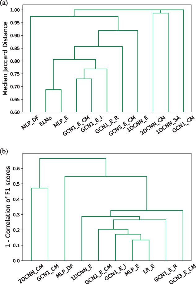
Hierarchical clustering of the models based on the similarity of the 40 nearest neighbors of each protein in the embedding space (a) and the correlation in protein-centric Fmax (b)
Finally, we investigated whether the observed differences in embeddings imply different performances across proteins. The clustering based on protein-centric performance (Fig. 3b) was very similar to the one obtained when using embedding similarities (Fig. 3a). The rank correlation between both similarities was 0.92. However, in absolute numbers, the performance similarities are much higher than the neighborhood similarities (at least 0.35 overall and at least 0.67 among methods that use ELMo embeddings). This shows that ELMo-based models tend to behave similarly.
4 Discussion
Our work continues upon two recent studies involving protein representation learning (Heinzinger et al., 2019) and its combination with protein structure applied to AFP (Gligorijevic et al., 2020). We confirm the power of the unsupervised ELMo embeddings in capturing relevant biological information about proteins (Heinzinger et al., 2019). Simply embedding the proteins into the learned 1024-dimensional space and applying the k-NN classifier led to better molecular function prediction performance than the two baseline methods (BLAST and naive), as well as several commonly used hand-crafted features such as one-hot encoding of amino acids, k-mer counts, secondary structure and backbone angles. This implies that the ELMo model was able to learn an embedding space in which the similarity between two proteins reflects functional similarity reasonably well, although it was only exposed to amino acid sequences and not to GO annotations. We had similar results with DeepFold embeddings (Liu et al., 2018) which model protein structures and a similar observation has been recently made for protein domain embeddings (Melidis et al., 2020). However, the ELMo representation only coarsely reflects protein function, as demonstrated by the poorer performance of the k-NN classifier on the most specific terms.
As expected, we were able to improve the prediction accuracy achieved by the unsupervised embeddings by training supervised AFP methods on the embedding space. A set of logistic regression classifiers trained individually for each GO term achieved comparable Smin and Fmax to the k-NN, while achieving significantly higher ROCAUC in the PDB dataset. Contrary to expectation, the GCN and 1D-CNN models trained on the amino acid-level embeddings extracted by ELMo were barely able to outperform the logistic regression model in terms of ROCAUC. They did outperform it in terms of Smin and Fmax, though. However, in the SP dataset, which is larger and contains more specific GO terms, the differences in Smin are less profound (Supplementary Table S7). Moreover, replacing the linear model (LR) with a non-linear one (MLP) gave a significant performance boost, considerably outperforming all others in ROCAUC and achieving competitive CAFA performance. Supervised training also resulted in a more consistent performance across all levels of GO term specificity. In contrast, for DeepFold embeddings, training supervised methods did not improve upon the k-NN performance. This is probably due to the fact that DeepFold is a metric learning model tuned to recognize similar protein structures and not to generally model protein characteristics. All in all, the competitive performance of the protein-level models highlights the power of the unsupervised protein embeddings.
In Gligorijevic et al. (2020), the authors report on the superiority of a 3-layer GCN using amino acid embeddings from a pretrained language model based on a LSTM network over BLAST and a 1D-CNN using a one-hot encoded amino acid representation. They attribute this superiority to the use of graph convolutions to model the protein 3D structure represented by contact maps. However, our experiments show that a 1D-CNN with strong amino acid embeddings is competitive with the GCN. Both convolutional models exhibited severe performance decline when replacing the ELMo embeddings with one-hot encoded amino acids. Based on these, we cannot exclude the possibility that the language model of Gligorijevic et al. (2020) is by itself powerful enough to explain (most of) the increase in performance. If that is indeed the case, it would account for the fact that replacing the true contact map with a predicted one does not cause a significant drop in performance Gligorijevic et al. (2020). To support this claim, we trained another GCN model from scratch, keeping the same architecture as our best GCN, but replacing the contact map by a graph with all nodes disconnected. The performance of that network was similar to that of the original (using the contact map). The same pattern was observed when replacing the contact map with a random graph (both at training and test time), clearly demonstrating that the contribution of the contact maps is rather small. This observation is interesting, as protein 3D structure is much more difficult and expensive to obtain than the sequence.
One of the hyperparameters of our networks was the number of fully connected (FC) layers between the global pooling layer and the output FC layer for the classification. In our experiments, we tested our models with zero and one intermediate FC layer and used the validation ROCAUC to select the optimal for each model. In cases where the performance difference was less than 0.01, we chose to keep the simpler model for testing, as having fewer parameters makes it less prone to overfitting and more likely to better generalize on unseen proteins. A clear pattern emerged from this selection: for both GCN and 1D-CNN networks trained with ELMo embeddings, the extra FC layer was not required. In contrast, for networks trained with one-hot encoded amino acid features or without any sequence features, the more complicated architecture was always selected. This means that in the feature space learned by the convolutional layers, the different classes (GO terms) are ‘more linearly separable’ when ELMo embeddings are used and learning a simple mapping from that space to the output classes is enough for good performance. In the absence of ‘good’ input features, it is harder for the convolutions to learn a ‘good’ embedding space and as a result a more complex classifier is needed.
One can reasonably assume that also in the case of the one-hot features, it would be possible to learn a better (supervised) embedding space that only requires one linear classification layer. However, that would take a deeper architecture with more convolutional layers to enable us to discover more complicated patterns in protein sequences. This is problematic because the amount of available labeled data is not enough to train deep models with a larger number of parameters. Our experiments showed that two recent models, a 3-layer GCN (Gligorijevic et al., 2020) and a wide 1D-CNN (Kulmanov and Hoehndorf, 2020), both operating on one-hot encoded amino acids, were remarkably inferior to linear and nearest neighbor methods that operate on pretrained features. Building a more complex model increases not only training time but also the man-hours spent deciding on the correct architecture and tuning the larger number of hyperparameters. To make matters worse, one would have to repeat almost the whole process from scratch if the task changes e.g. from function prediction to structure prediction. Unsupervised pretraining relieves part of that burden by creating only one complicated deep sequence model to learn a meaningful feature representation of amino acids or proteins, which can then be fed to simpler classifiers to obtain competitive performance in several tasks without much effort (Heinzinger et al., 2019), as we demonstrated here.
Note that, DeepGOCNN combined with other data sources performed better on the CAFA3 MFO benchmark than our MLP_E model (Kulmanov and Hoehndorf, 2020). Here, we focused on combining ELMo with protein structure information, but other, more diverse data types such as coexpression and protein interactions should be tested in conjunction with these advanced sequence features in ensemble methods. We expect this to be highly beneficial in the BPO, because ELMo did not achieve high CAFA3 performance in that ontology and the CAFA-π results hinted that achieving good BPO performance using sequence alone is difficult (Zhou et al., 2019).
Our experiments suggest that combining structure information in the form of a contact map with sequence information is not straightforward, when high-quality sequence features are available. Joining a 1D- and a 2D-CNN that independently extract sequence and contact map features, respectively, did not improve performance over the 1D-CNN applied to sequence data only. It is unlikely that contact maps do not contain any functional information, so our observations could have two possible explanations: either the ELMo embeddings contain 3D structure information or we are still unable to leverage the full potential of contact maps.
To test the first hypothesis, one could train a classifier that takes the amino acid-level features as inputs and predicts contacts between amino acid pairs. Such models already exist and do quite well in the CASP challenges using physicochemical properties, the position-specific scoring matrix (PSSM) and predictions about secondary structure, solvent accessibility and backbone angles (Cheng and Baldi, 2007; Jones et al., 2015; Wang et al., 2017). By replacing these features with sequence embeddings as in Bepler and Berger (2019), we would expect a considerable improvement in the performance of these models.
On the contrary, finding a more effective way of using distance or contact maps is not trivial. Here, we considered a contact threshold of 10 Å by following previous studies (Gligorijevic et al., 2020), which is a more relaxed threshold than the one used in CASP challenges (8 Å), but also used alternative threshold strategies and obtained similar results. One could argue that the distance matrix is more informative and should be preferred, but our experiments did not confirm that. A different way of using distance maps in a GCN has been proposed by Fout et al. (2017) to predict protein interfaces. First, instead of using a fixed distance threshold, Fout et al. define each amino acid as being ‘in contact’ with its k-nearest residues, which creates a directed graph as the property of being someone’s nearest neighbor is not commutative. Moreover, the distances between the k-nearest residues were smoothed with a Gaussian kernel and used as edge features over which a different set of filters was learned (Fout et al., 2017). Further research is required to resolve this issue, but our DeepFold results show that unsupervised pretraining is a promising path in this case too.
In conclusion, this study shows that deep unsupervised pretraining of protein sequences is beneficial for predicting molecular function, as it can capture useful aspects of the amino acid sequences. We also showed that combining these sequential embeddings with contact map information does not yield significant performance improvements in the task, hinting that the embeddings may already contain 3D structural information. As language modeling of proteins is a new field with great potential, we think that future work should perform systematic comparisons of those models in AFP, but also other protein-related tasks.
Supplementary Material
Acknowledgements
The authors thank Dr. Elvin Isufi and Chirag Raman for their valuable comments and feedback.
Funding
This work was supported by Keygene N.V., a crop innovation company in the Netherlands and by the Spanish MINECO/FEDER Project TEC2016-80141-P with the associated FPI grant BES-2017-079792.
Conflict of Interest: none declared.
References
- Alley E.C. et al. (2019) Unified rational protein engineering with sequence-based deep representation learning. Nat. Methods, 16, 1315–1322. [DOI] [PMC free article] [PubMed] [Google Scholar]
- Altschul S.F. et al. (1990) Basic local alignment search tool. J. Mol. Biol., 215, 403–410. [DOI] [PubMed] [Google Scholar]
- Anfinsen C.B. (1973) Principles that govern the folding of protein chains. Science, 181, 223–230. [DOI] [PubMed] [Google Scholar]
- Ashburner M. et al. (2000) Gene ontology: tool for the unification of biology. Nat. Genet., 25, 25–29. [DOI] [PMC free article] [PubMed] [Google Scholar]
- Bartoli L. et al. (2007) The pros and cons of predicting protein contact maps. Methods Mol. Biol., 413, 199–217. [DOI] [PubMed] [Google Scholar]
- Bepler T., Berger B. (2019). Learning protein sequence embeddings using information from structure. In 7th International Conference on Learning Representations, ICLR 2019. OpenReview.net. Massachusetts, USA.
- Berman H.M. et al. (2000) The Protein Data Bank (www.rcsb.org). Nucleic Acids Res., 43, 235–242. [DOI] [PMC free article] [PubMed] [Google Scholar]
- Bonetta R., Valentino G. (2020) Machine learning techniques for protein function prediction. Proteins Struct. Funct. Bioinf., 88, 397–413. [DOI] [PubMed] [Google Scholar]
- Cao R. et al. (2017) ProLanGO: protein function prediction using neural machine translation based on a recurrent neural network. Molecules, 22, 1732. [DOI] [PMC free article] [PubMed] [Google Scholar]
- Cheng J., Baldi P. (2007) Improved residue contact prediction using support vector machines and a large feature set. BMC Bioinformatics, 8.113. [DOI] [PMC free article] [PubMed] [Google Scholar]
- Clark W.T., Radivojac P. (2013) Information-theoretic evaluation of predicted ontological annotations. Bioinformatics, 29, i53–61. [DOI] [PMC free article] [PubMed] [Google Scholar]
- Cozzetto D. et al. (2016) FFPred 3: feature-based function prediction for all Gene Ontology domains. Sci. Rep., 6, 31865. [DOI] [PMC free article] [PubMed] [Google Scholar]
- Devlin J. et al. (2018) Bert: pre-training of deep bidirectional transformers for language understanding. arXiv preprint arXiv : 1810.04805.
- Doersch C. et al. (2015) Unsupervised visual representation learning by context prediction. In: 2015 IEEE International Conference on Computer Vision (ICCV), IEEE Computer Society, USA, pp. 1422–1430.
- dom2vec: Unsupervised protein domain embeddings capture domains structure and function providing data-driven insights into collocations in domain architectures. bioRxiv, 2020.03.17.995498.
- Duarte J.M. et al. (2010) Optimal contact definition for reconstruction of Contact Maps. BMC Bioinformatics, 11. 1-10. [DOI] [PMC free article] [PubMed] [Google Scholar]
- Eddy S.R. (2009) A new generation of homology search tools based on probabilistic inference. In: International Conference on Genome Informatics. Imperial College Press, London, UK. [PubMed]
- Fa R. et al. (2018) Predicting human protein function with multitask deep neural networks. PLoS One, 13, e0198216. [DOI] [PMC free article] [PubMed] [Google Scholar]
- Fout A. et al. (2017) Protein interface prediction using graph convolutional networks. In: Advances in Neural Information Processing Systems, Vol. 30. Curran Associates, Inc., Red Hook, NY, USA , pp. 6530–6539. [Google Scholar]
- Fu L. et al. (2012) CD-HIT: accelerated for clustering the next-generation sequencing data. Bioinformatics, 28, 3150–3152. [DOI] [PMC free article] [PubMed] [Google Scholar]
- Gidaris S. et al. (2018) Unsupervised representation learning by predicting image rotations. ArXiv, abs/1803.0.
- Gligorijevic V. et al. (2020) Structure-based function prediction using graph convolutional networks. bioRxiv. [DOI] [PMC free article] [PubMed]
- Heinzinger M. et al. (2019) Modeling aspects of the language of life through transfer-learning protein sequences. BMC Bioinformatics, 20, 723. [DOI] [PMC free article] [PubMed] [Google Scholar]
- Jiang Y. et al. (2016) An expanded evaluation of protein function prediction methods shows an improvement in accuracy. Genome Biol., 17, 184. [DOI] [PMC free article] [PubMed] [Google Scholar]
- Jones D.T. et al. (2015) MetaPSICOV: combining coevolution methods for accurate prediction of contacts and long range hydrogen bonding in proteins. Bioinformatics, 31, 999–1006. [DOI] [PMC free article] [PubMed] [Google Scholar]
- Kabsch W., Sander C. (1983) Dictionary of protein secondary structure: pattern recognition of hydrogen-bonded and geometrical features. Biopolym. Orig. Res. Biomol., 22, 2577–2637. [DOI] [PubMed] [Google Scholar]
- Kane H. et al. (2019) Augmenting protein network embeddings with sequence information. BioRxiv, 730481.
- Kimura M., Ohta T. (1974) On some principles governing molecular evolution. Proc. Natl. Acad. Sci. USA, 71, 2848–2852. [DOI] [PMC free article] [PubMed] [Google Scholar]
- Kingma D.P., Ba J.L. (2015) Adam: a method for stochastic optimization. In: 3rd International Conference on Learning Representations, ICLR 2015– Conference Track Proceedings. Ithaca, NY, USA.
- Kipf T.N., Welling M. (2019) Semi-supervised classification with graph convolutional networks. In: 5th International Conference on Learning Representations, ICLR 2017 – Conference Track Proceedings. OpenReview.net. Massachusetts, USA.
- Kulmanov M., Hoehndorf R. (2020) DeepGOPlus: improved protein function prediction from sequence. Bioinformatics, 36, 422–429. [DOI] [PMC free article] [PubMed] [Google Scholar]
- Kulmanov M. et al. (2018) DeepGO: predicting protein functions from sequence and interactions using a deep ontology-aware classifier. Bioinformatics, 34, 660–668. [DOI] [PMC free article] [PubMed] [Google Scholar]
- Liu X. (2017) Deep recurrent neural network for protein function prediction from sequence. arXiv preprint arXiv: 1701.08318.
- Liu Y. et al. (2018) Learning structural motif representations for efficient protein structure search. Bioinformatics, 34, i773–i780. [DOI] [PMC free article] [PubMed] [Google Scholar]
- Lyons J. et al. (2014) Predicting backbone Ca angles and dihedrals from protein sequences by stacked sparse auto-encoder deep neural network. J. Comput. Chem., 35, 2040–2046. [DOI] [PubMed] [Google Scholar]
- Mathis A. et al. (2019) Pretraining boosts out-of-domain robustness for pose estimation. ArXiv, abs/1909.1.
- McCann B. et al. (2017) Learned in translation: contextualized word vectors. In: Advances in Neural Information Processing Systems. Neural Information Processing Systems. San Diego, CA, USA.
- Pesquita C. et al. (2007) Evaluating GO-based semantic similarity measures. In Proc. 10th Annual Bio-Ontologies Meeting.
- Peters M. et al. (2018) Deep contextualized word representations. arXiv preprint arXiv: 1802.05365.
- Radivojac P. et al. (2013) A large-scale evaluation of computational protein function prediction. Nat. Methods, 10, 221–227. [DOI] [PMC free article] [PubMed] [Google Scholar]
- Rao R. et al. (2019) Evaluating protein transfer learning with tape. In: Wallach H.et al. (eds.) Advances in Neural Information Processing Systems, Vol. 32. Curran Associates, Inc., Red Hook, NY, USA, pp. 9689–9701 [PMC free article] [PubMed] [Google Scholar]
- Rives A. et al. (2019) Biological structure and function emerge from scaling unsupervised learning to 250 million protein sequences. bioRxiv. [DOI] [PMC free article] [PubMed]
- Srivastava N. et al. (2014) Dropout: a simple way to prevent neural networks from overfitting. J. Mach. Learn. Res., 15, 1929–1958. [Google Scholar]
- Sureyya Rifaioglu A. et al. (2019) DEEPred: automated protein function prediction with multi-task feed-forward deep neural networks. Sci. Rep., 9, 1–16. [DOI] [PMC free article] [PubMed] [Google Scholar]
- Wang S. et al. (2017) Accurate De Novo prediction of protein contact map by ultra-deep learning model. PLoS Comput. Biol., 13, e1005324. [DOI] [PMC free article] [PubMed] [Google Scholar]
- Weinhold N. et al. (2008) Local function conservation in sequence and structure space. PLoS Comput. Biol., 4, e1000105. [DOI] [PMC free article] [PubMed] [Google Scholar]
- Wilson C.A. et al. (2000) Assessing annotation transfer for genomics: quantifying the relations between protein sequence, structure and function through traditional and probabilistic scores. J. Mol. Biol., 297, 233–249. [DOI] [PubMed] [Google Scholar]
- Zamora-Resendiz R., Crivelli S. (2019) Structural learning of proteins using graph convolutional neural networks. bioRxiv, 610444.
- Zheng W. et al. (2019) Detecting distant-homology protein structures by aligning deep neural-network based contact maps. PLoS Comput. Biol., 15, e1007411. [DOI] [PMC free article] [PubMed] [Google Scholar]
- Zhou N. et al. (2019) The CAFA challenge reports improved protein function prediction and new functional annotations for hundreds of genes through experimental screens. Genome Biol., 20, 244. [DOI] [PMC free article] [PubMed] [Google Scholar]
- Zhu J. et al. (2017) Improving protein fold recognition by extracting fold-specific features from predicted residue–residue contacts. Bioinformatics, 33, 3749–3757. [DOI] [PubMed] [Google Scholar]
Associated Data
This section collects any data citations, data availability statements, or supplementary materials included in this article.