

Abstract
Summary
Large-scale transcriptome studies with multiple samples per individual are widely used to study disease biology. Yet, current methods for differential expression are inadequate for cross-individual testing for these repeated measures designs. Most problematic, we observe across multiple datasets that current methods can give reproducible false-positive findings that are driven by genetic regulation of gene expression, yet are unrelated to the trait of interest. Here, we introduce a statistical software package, dream, that increases power, controls the false positive rate, enables multiple types of hypothesis tests, and integrates with standard workflows. In 12 analyses in 6 independent datasets, dream yields biological insight not found with existing software while addressing the issue of reproducible false-positive findings.
Availability and implementation
Dream is available within the variancePartition Bioconductor package at http://bioconductor.org/packages/variancePartition.
Contact
gabriel.hoffman@mssm.edu
Supplementary information
Supplementary data are available at Bioinformatics online.
1 Introduction
Transcriptome profiling and comparison of gene expression levels are a widely used genomic technique in biomedical research. In a typical study, a researcher collects gene expression by RNA-seq or microarray from multiple samples and performs differential expression analysis between subsets of samples that differ in cell/tissue type, environmental conditions, stimuli, genotype or disease state. A range of statistical methods have been developed for this purpose and give state-of-the-art performance on this typical study design (Chowdhury et al., 2018; Costa-Silva et al., 2017; Law et al., 2014; Love et al., 2014; Pimentel et al., 2017; Ritchie et al., 2015; Robinson et al., 2010; Tarazona et al., 2015; Yu et al., 2017, 2019).
Recent advances in the scale of transcriptomic and, more generally, functional genomic studies have enabled assaying individuals from multiple tissues (Aguet et al., 2017; Franzén et al., 2016), brain regions (Wang et al., 2018; Zhang et al., 2013), cell types (Van Der Wijst et al., 2018), time points (Alasoo et al., 2018; Breen et al., 2015) or induced pluripotent stem cell (iPSC) lines (Carcamo-Orive et al., 2017; Hoffman et al., 2017; Mariani et al., 2015; Paşca et al., 2011; Schwartzentruber et al., 2018; Warren et al., 2017). These studies with multiple samples from each individual can test region- or context-specific effects, but can also increase the statistical power to detect effects that are shared by multiple replicates (Hoffman et al., 2017, 2019; Pinheiro and Bates, 2000). Collecting replicates also enables samples from the same individual to be processed in multiple technical batches to decouple biological from technical variation in gene expression (Blainey et al., 2014). Finally, collecting replicates can also be beneficial when gene expression measurements are noisy, when expression is dynamic or stochastic, or when adding additional individuals is not feasible (Blainey et al., 2014; Hoffman et al., 2017).
In a standard case/control study of gene expression with only one sample per individual, typical analysis tests the expression differences between case and control individuals. However, in repeated measures designs with two or more samples per individual, analysis can perform three types of statistical tests: (i) within-individual, (ii) a combination of within- and cross-individual and (iii) cross-individual. Within-individual analysis uses an individual-specific baseline to, for example, examine time-course data to identify a differential expression signature of stimulus response, or identify individual-specific expression differences between two cell types each measured in the same set of individuals. In this case, the analysis focuses on the differences between the samples from the same individual, and the repeated measures from the same individual capture distinct biology. The simplest form of within-individual analysis is a paired t-test. The combined within- and cross-individual analysis, evaluates within-individual differences between, for example, two time points and then compares the results between cases and controls. Standard RNA-seq software (Law et al., 2014; Love et al., 2014; Pimentel et al., 2017; Ritchie et al., 2015; Robinson et al., 2010; Tarazona et al., 2015) that model these data with fixed effects terms perform well. Alternatively, software using linear mixed models specifically designed for longitudinal analysis of transcriptomic data can be applied (Straube et al., 2015).
We focus here on cross-individual analysis that considers the shared biology of the multiple samples from the same individual. For example, multiple iPSC lines can be generated from the same individual as biological replicates, or multiple brain regions can be assayed from each individual in a case/control study. The repeated measures design can be leveraged to account for biological and technical variability, and model the shared biology of these replicates to increase the statistical power to identify differentially expressed genes. In this case, the multiple replicates from the same individual are considered to be statistically exchangeable after accounting for variation due to covariates such as tissue type, region or technical factors. Since all replicates from the same individual have the same phenotype of interest (i.e. disease status), modeling individual as a fixed effect is not possible because the individual effect is perfectly confounded with the phenotype of interest. Statistically, a fixed effect regression model cannot be fit when the design matrix is not invertible and so parameter estimation and hypothesis testing cannot be performed (Rencher and Schaalje, 2008). Therefore, individual must either be modeled as a random effect (Pinheiro and Bates, 2000), or the multiple samples from each individual must be collapsed into an individual-level summary.
While summing reads from the multiple samples from the same individual is a simple way to analyze repeated measures data, it has a number of issues. At a basic level, it applies equal weight to each individual even though some may have five samples while others have only two. More problematic is the fact that summing reads ignores any biological or technical differences between the multiple samples from the same individual. Some samples may have been processed in a different technical batch, or come from a different tissue or region. Many methods can account for these differences in the full dataset (Johnson et al., 2007; Leek and Storey, 2007; Stegle et al., 2010), but summing the reads loses this information about within-individual variation.
Moreover, analysts are often interested in tests that allow for heterogeneity of effect sizes within subsets of samples and then perform a joint test of multiple coefficients. For example, in a case/control study of three brain regions, it may be of interest to allow the case/control effect to vary between brain regions and then perform a joint test of case/control effects with three degrees of freedom with an F-test. Obviously, collapsing read counts at the individual level is not compatible with this type of analysis.
Despite the potential of leveraging cross-individual analysis in repeated measures designs, standard differential expression methods do not adequately model the complexity of these repeated measures study designs (Law et al., 2014; Love et al., 2014; Pimentel et al., 2017; Ritchie et al., 2015; Robinson et al., 2010; Tarazona et al., 2015). Recent work has emphasized that applying current methods to cross-individual analysis of repeated measures datasets can result in loss of power or, more problematically, a large number of false-positive findings (Germain and Testa, 2017; Jostins et al., 2012). The advantages of repeated measures designs cannot be realized without the proper statistical methods and software.
Statistically, repeated measures data are problematic for existing software because samples from the same individual are correlated, while existing methods assume statistical independence between samples after correcting for covariates. Following our previous work on repeated measures data in genomics (Carcamo-Orive et al., 2017; Girdhar et al., 2018; Hoffman and Schadt, 2016; Hoffman et al., 2017), this correlation between samples from the same individual can be quantified in terms of the fraction of expression variance explained by variance across individuals. Genes with high variance across individuals are expressed at similar levels within replicates from the same individual. This departure from statistical independence is substantial and must be considered in any statistical test.
To perform differential expression testing while accounting for this correlation structure, some analysts have adopted the duplicateCorrelation method in the limma workflow (Germain and Testa, 2017; Ritchie et al., 2015). Although originally designed for replicate probes in microarrays (Smyth et al., 2005), this method has been applied ‘off-label’ to repeated measures study designs (Ritchie et al., 2015). Its adoption has been driven in part by its seamless integration with limma. In the duplicateCorrelation model, the correlation between replicates from the same individual for gene g is denoted by and is estimated using a linear mixed model. The duplicateCorrelation method uses a single value genome-wide, , and assumes that the correlation structure for every gene is the same. While this assumption is necessary for dealing with small datasets, current transcriptomic datasets are sufficiently large that this modeling approach is problematic. In fact, Germain and Testa (2017) reported that duplicateCorrelation reduces the false-positive rate in simulations using real RNA-seq data.
Using a single value, , genome-wide for the correlation within individuals can reduce power and increase the false-positive rate in a particular, reproducible way. Consider the correlation value for gene g, , compared to the single genome-wide value, . When testing a variable that is constant for all replicates of an individual, for genes where , using under-corrects for the correlation within individuals so that it increases the false-positive rate of gene g compared to using . Conversely, for genes where , using over-corrects for the correlation within individuals so that it decreases power for gene g. Increasing sample size does not overcome this issue.
While the use of gene-level random effects has been proposed previously in methodological work, a number of significant hurdles have prevented wider adoption by analysts. Existing methods are either very computational demanding, do not model error structure of RNA-seq data, do not fit easily into existing workflows, or require extensive knowledge of the theory of linear mixed models and details of implementing these models in R. macau2 (Sun et al., 2017) fits a Poisson mixed model for count data for RNA-seq and uses a single random effect to account for multiple samples from the same individual using a pairwise similarity matrix. However, this method does not allow multiple random effects, is not able to fit over-dispersed count models widely used for RNA-seq data (Law et al., 2014; Love et al., 2014; Robinson et al., 2010), and is not scalable to large datasets. Trabzuni and Thomson (2014) proposed a method that fits all of the genes jointly in a linear mixed model, estimates a random effect term modeling the gene by disease interaction, and then considers a genome-wide mixture model of the variance estimates to identify differentially expressed genes. However, this approach does not model count data, is very computationally demanding, and is fit with the commercial package ASReml-R (Butler et al., 2018). Bryois et al. (2017) applied a linear mixed model to differential expression of RNA-seq data, but do not consider the count-nature of the data and do not provide software. Recently, Yu et al. (2019) proposed a fully moderated t-statistic (FMT) that extends the empirical Bayes method of Smyth (2004) to linear mixed models, but application by non-specialists is challenging.
While a number of generic statistical methods for estimation and hypothesis for testing linear mixed models are available (Bates et al., 2015; Kuznetsova et al., 2017; Pinheiro and Bates, 2000), practical application of these methods to RNA-seq data has been limited due to the challenges of (i) implementing these methods for each dataset, (ii) high computational cost to fit linear mixed models, (iii) directly modeling count data and (iv) uncertainty about the conditions where linear mixed models with gene-level variance terms will outperform existing methods.
Here, we present a statistical software package, dream (differential expression for repeated measures), that addresses each of these hurdles by leveraging multiple open-source R packages (described below) and outperforms existing methods for cross-individual tests in repeated measures datasets.
2 Materials and methods
Linear mixed models are commonly applied in biostatistics to account for the correlation between observations from the same individual in repeated measures studies (Laird and Ware, 1982; Pinheiro and Bates, 2000). An array of linear mixed models have been applied to gene expression studies (Bryois et al., 2017; Carcamo-Orive et al., 2017; Germain and Testa, 2017; Hoffman and Schadt, 2016; Hoffman et al., 2017; Ritchie et al., 2015; Smyth et al., 2005; Straube et al., 2015; Sun et al., 2017; Trabzuni and Thomson, 2014; Warren et al., 2017) in recent years and are reviewed above. We start with a description of a simple linear model for differential expression analysis and build towards the dream model.
2.1 Linear models for differential expression
Consider a linear model for a single gene
| (1) |
where yg is a vector of counts per million for gene g, the matrix X stores covariates as columns, βg is the vector of regression coefficients and is normally distributed error. In order to account for heteroskedastic error from RNA-seq counts, the error takes the form
| (2) |
where is the residual variance, and wg is a vector of precision weights (Law et al., 2014). Precision weights can be learned from the data to account for counting error in RNA-seq or variation in sample quality (Law et al., 2014; Ritchie et al., 2015). In this case, the estimates can be obtained by a closed form least squares model fit. Hypothesis testing is performed by specifying a contrast matrix L that is a linear combination of the estimated coefficients and evaluating the null model
| (3) |
Alternatively, an F-test jointly testing multiple coefficients can be applied.
2.1.1 Accounting for repeated measures with a two-step model: duplicateCorrelation
The most widely used approach for handing repeated measures in differential expression analysis is the duplicateCorrelation() function available in limma (Ritchie et al., 2015). This approach involves two steps. In the first step, a linear mixed model is fit for each gene separately, and only allows a single random effect. The model is
| (4) |
| (5) |
where Z is the design matrix for the random effect, with coefficients αg drawn from a normal distribution with variance . After fitting this model for each gene, a single genome-wide variance term is computed according to
| (6) |
where G is the number of genes, tanh is the hyperbolic tangent and atanh is its inverse.
In the next step, this single variance term, , is then used in a generalized least squares model fit for each gene, blocking by individual:
| (7) |
| (8) |
| (9) |
where is the covariance between samples and considers the correlation between samples from the same individual. Note that, the same value is used for all genes.
The duplicateCorrelation method allows the user to specify a single random effect usually corresponding to donor. So, it cannot model multilevel design. Moreover, duplicateCorrelation estimates a single variance term genome-wide even though the donor contribution of a particular gene can vary substantially from the genome-wide trend (Hoffman and Schadt, 2016). Using a single value genome-wide for the within-donor variance can reduce power and increase the false-positive rate in a particular, reproducible way as described in Section 1.
Using the single variance term genome-wide and using the tanh and atanh are designed to address the high estimation uncertainly for small gene expression experiments. However, using this single variance term has distinct limitations. First, it ignores the fact that the contribution of the random effect often varies widely from gene to gene (Hoffman and Schadt, 2016). Using a single variance term to account for the correlation between samples from the same individuals over-corrects for this correlation for some genes and under-corrects for others. In addition, it is a two-step approach that first estimates the variance term and then estimates the regression coefficients. Thus, it does not account for the statistical uncertainty in the estimate of . Finally, it does not account for the fact that estimating the variance component changes the null distribution of . Specifically, estimating variance components in a linear mixed model can substantially change the degrees of freedom of the distribution used to approximate the null distribution for fixed effect coefficients (Giesbrecht and Burns, 1985; Halekoh and Højsgaard, 2014; Hoffman, 2013; Kenward and Roger, 1997; Kuznetsova et al., 2017). Ignoring this issue can lead to false positive differentially expressed genes.
2.1.2 Dream model
The dream model extends the previous model to enable multiple random effects, enable the variance terms to vary across genes, and approximate degrees of freedom of hypothesis test for each gene and contrast from the data to reduce false positive. The definition of the dream model follows directly from the definition of the previous models. First, consider a linear mixed model for gene g with an arbitrary number of random effects:
| (10) |
| (11) |
where Zj is the design matrix for the jth random effect, with coefficients drawn from a normal distribution with variance . As before, heteroskedastic errors are modeled with precision weights with
| (12) |
In this case, estimates of coefficients and variance components must be obtained via an iterative optimization algorithm (Bates et al., 2015).
For the linear model and generalized least squares model described above, the degrees of freedom of the hypothesis test is fixed at N – p, where N is the number of samples, and p is the number of covariates.
See Supplementary Methods for estimation of the approximate degrees of freedom for the hypothesis test, and modeling precision weights in the linear mixed model.
2.1.3 Features of dream
Dream enables powerful analysis of repeated measures data while properly controlling the false positive rate. Dream leverages open-source R packages to combine the following features in an efficient and user-friendly workflow:
random effects estimated separately for each gene: variancePartition (Hoffman and Schadt, 2016)
ability to model multiple random effects: lme4 (Bates et al., 2015)
fast hypothesis testing for fixed effects in linear mixed models including:
tests of single coefficients
linear contrasts specifying a linear combination of coefficients
joint hypothesis testing of multiple coefficients using an F-test lmerTest (Kuznetsova et al., 2017)
small sample size Kenward–Roger hypothesis test to increase power: pbkrtest (Halekoh and Højsgaard, 2014)
precision weights to model measurement error in RNA-seq counts: limma::voom (Law et al., 2014)
seamless integration with the widely used workflow of limma: limma (Ritchie et al., 2015)
parallel processing on multicore machines with efficient memory usage: BiocParallel, iterators (Morgan et al., 2019; Ooi and Weston, 2019)
See Supplementary Methods for details about software, implementation, simulation and data analysis.
3 Results
3.1 Biologically motivated simulations demonstrate performance of dream
The performance of dream was compared to current methods on biologically motivated simulations that were designed to reproduce some of the properties observed in real data (see Supplementary Methods). The methods can be divided into six categories:
dream (i) using default settings, (ii) a Kenward–Roger (KR) approximation that is more powerful but much more computationally demanding, (iii) a fully moderated t-statistic (FMT) (Yu et al., 2019) using either a variance component (vc) or Welch–Satterthwaite (ws) to estimate the degrees of freedom of the test
duplicateCorrelation from the limma/voom workflow (Ritchie et al., 2015)
macau2 (Sun et al., 2017)
In addition, DESeq2 (Love et al., 2014) and limma/voom(Law et al., 2014) serve as representatives of differential expression methods that do not directly consider repeated measures designs and are run:
including all samples but ignoring the repeated measures design
with only a single replicate per individual
summing the reads across biological replicates from the same individual
Two dream methods (default and KR) are more powerful than the other methods (Fig. 1). Across a range of simulations of 4–50 individuals each with 2–4 biological replicates, these two dream methods have a lower false-discovery rate (Fig. 1A, Supplementary Fig. S1), better precision–recall curves (Fig. 1B, Supplementary Fig. S2) and larger area under the precision–recall (AUPR) curve (Fig. 1C, Supplementary Fig. S3). The fully moderated t-statistics methods (FMT.vc and FTM.ws) had slightly lower AUPR, but, more importantly, did not control the false-positive rate. A test of differential expression must control the false-positive rate accurately to be useful in practice. As expected (Germain and Testa, 2017; Jostins et al., 2012), the methods that include all samples but ignore the correlation structure do not control the false-positive rate (Fig. 1D). Importantly, analysis that sums reads from multiple replicates controls the false-positive rate as expected, and has better power than using only a single replicate. Yet summing has lower power than methods that model the correlation structure of the full dataset. Aggregating results across many simulation conditions reveals trends as the number of individuals and replicates increases (Fig. 2). The lack of type I error control for methods that ignore the correlation structure, as well as macau2, is present in all simulation conditions (Fig. 2A, Supplementary Fig. S4). Even more concerning, increasing the number of repeated measures can dramatically increase the false-positive rate. Notably, duplicateCorrelation shows a slight increase in type I error at larger sample sizes. For macau2, the type I error is very inflated for small samples sizes but decreases for larger datasets. Higher type I error can translate into hundreds of false positive differentially expressed genes even when no genes are truly differently expressed (Fig. 2B). Importantly, both versions of dream accurately control the type I error with sufficient sample size.
Fig. 1.

Performance on biologically motivated simulated data. (A, B, C, D) Performance from 50 simulations of RNA-seq datasets of 14 individuals each with 3 replicates. (A) False discoveries plotted against the number of genes called differentially expressed by each method. (B) Precision–recall curve showing performance in identifying true differentially expressed genes. Dashed line indicates performance of a random classifier. (C) Area under the precision–recall (AUPR) curves from (B). Dashed line indicates AUPR of a random classifier. Error bars indicate 95% confidence intervals, and we note that the intervals are very small. (D) False positive rate at P < 0.05 evaluated under a null model were no genes are differentially expressed illustrates calibration of type I error from each method. As indicated by the dashed line, a well calibrated method should give P-values < 0.05 for 5% of tests under a null model
Fig. 2.

Performance summary for simulations with a range of individuals and replicates. Simulations were performed on 4–50 individuals with between 2 and 4 replicates. For each condition, 50 simulations were performed for a total of 1800. (A) False-positive rate at P < 0.05 for simulations versus the number of individuals and replicates. Black dashed line indicates target type I error rate of 0.05. (B) Number of genes passing FDR cutoff of 5% under the null simulations. Values shown are averaged across 50 simulations. (C) AUPR for simulations versus the number of individuals and replicates
Two versions of dream (default and KR) give the highest AUPR across all simulation conditions (Fig. 2C) while properly controlling the false-positive rate. In addition, macau2 also produces a competitive AUPR, but lack of type I error control and high computational cost is problematic (Supplementary Fig. S5A). While dream-KR gives the best performance, especially at small sample sizes, the computational time required can be prohibitive. Using dream with the default settings performs nearly as well in simulations, but can be 2–20× faster (Fig. 3, Supplementary Fig. S5B). For datasets with greater than 500 individuals, dream is also 5–10× faster than duplicateCorrelation. The tradeoff between statistical performance and computational time is an important factor when deciding which method to apply to real data. We note that macau2, dream-KR and duplicateCorrelation all have quadratic time complexity with respect to the number of samples, while all other methods are linear time. In practice, macau2 and dream-KR are the most time intensive, followed by dream which is substantially faster (Fig. 3, Supplementary Fig. S5A). Finally, FMT.vc and FMT.ws are post-processing steps based on the results of dream that require <5 additional seconds.
Fig. 3.
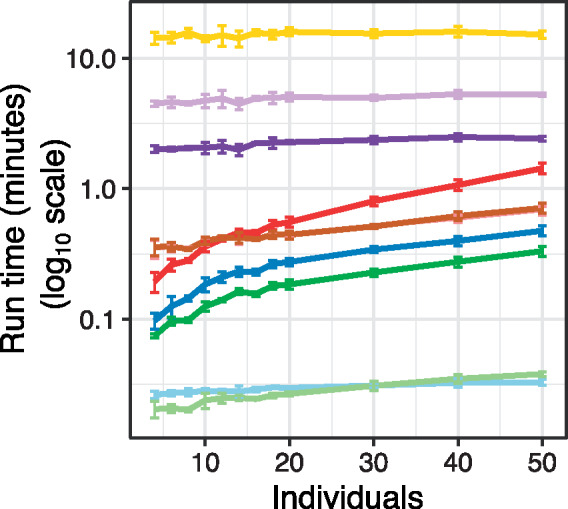
Run time for each method as the number of individuals increases. Times are shown for simulations in Figure 2 with three replicates per individual. Colors are same as for previous figure. Error bars indicate 95% confidence interval. We note that times for dream + FMT.vc and dream + FMT.ws are omitted here because they are post-processing steps based on the results of dream that require <5 additional seconds
3.2 Null simulations using real RNA-seq data
Since simulated counts cannot fully reproduce the biological, technical and random variability of real data, we used counts from 317 RNA-seq samples of induced pluripotent stem cells from 101 individuals (Carcamo-Orive et al., 2017). Subsets of the data were generated using individuals and replicates per individual. A continuous variable to be the focus of the differential expression analysis was simulated for each sample. For this purpose, a normally distributed variable independent of the gene expression data was simulated with 99% of the variance across individuals and 1% of the variance within individuals. (We note that simulating binary values for this variable gives similar results.) For each (N, R) pair five independent simulations were performed and the results were aggregated.
The dream-KR method gave the most accurate control of false-positive rate across all simulations, and dream with default settings performed well with individuals (Supplementary Figs S6, S7). Post-processing with FMT.vc or FMT.ws gave too many small P-values for small N and too few small P-values for larger N. As expected, ignoring this correlation structure with limma for DESeq2 gave inflated false-positive rate in all conditions. The duplicatedCorrelation method and macau2 give increased false-positive rate for small N. Using a single replicate per individual or summing reads across replicates accurately controlled the false-positive rate with sufficient sample size.
Since count magnitude is related to the amount of measurement error, inadequate modeling of the uncertainty can result in a false-positive rate related to count magnitude (Young et al., 2010). While the simulations indicate an increased false-positive rate with increased counts per million for many methods, dream using default settings or KR gave accurate control of false-positive rate across the range of expression magnitudes for N > 5 (Supplementary Fig. S8).
3.3 Analysis of expression profiling datasets with dream gives biological insight
Applying dream to empirical data gives biological insight for three neuropsychiatric diseases with different genetic architectures. To avoid using arbitrary P-value or FDR cutoffs to identify differentially expressed genes, gene set enrichments were evaluated using cameraPR (Ritchie et al., 2015; Wu and Smyth, 2012) to compare the differential expression test statistics from genes in a given gene set to the genome-wide test statistics.
Alzheimer’s disease is a common neurodegenerative disorder with a complex genetic architecture (Lambert et al., 2013)(Fig. 4). In analysis of RNA-seq data from 4 regions of post-mortem brains from 26 individuals (Wang et al., 2018), dream identified known patterns of dysregulation in genes involved in adipogenesis, inflammation and monocyte response associated with Braak stage, a neuropathological metric of disease progression (Fig. 4A, Supplementary Fig. S9). Here, we allow the disease effect to be different in each brain region and then test if the sum of the four coefficients is significantly different from zero using a linear contrast. Applying duplicateCorrelation only recovered a subset of these findings and produced larger false-discovery rates across many biologically relevant gene sets. Notably, the difference between dream and duplicateCorrelation is due to the way that these methods account for expression variation explained by variance across individuals (Fig. 4B). Genes with correlation within individuals, , that is larger than the genome-wide average, , are susceptible to being called as false positive differentially expressed genes by duplicateCorrelation. Conversely if , then dream will tend to give a more significant P-value than duplicateCorrelation. For example, consider TUBB2B where compared to the genome-wide . Here, duplicateCorrelation under-corrects for the correlation structure and gives a P-value of 1.3e-10 while dream uses a gene-specific correlation to give P-value of only 7.7e-4 (Fig. 4C). Finally, we note that performing a joint F-test of these coefficients with four degrees of freedom gives similar results (Supplementary Fig. S10).
Fig. 4.

Application to transcriptome data from Alzheimer’s disease. (A) Gene set enrichment FDR for genes associated with Braak stage. Results are shown for dream and duplicateCorrelation. Lines with broad and narrow dashes indicate 10% and 5% FDR cutoff, respectively. (B) Comparison of P-values from applying dream and duplicateCorrelation to Braak stage. Each point is a gene, and is colored by the fraction of expression variation explained by variance across individuals. Black solid line indicates a slope of 1. Dashed line indicates the best fit line for the 20% of genes with the highest (red) and lowest (blue) expression variation explained by variance across individuals. (C) Expression of TUBB2B stratified by individual and colored by Braak stage so that each box represents the expression in the multiple samples from a given individual. Bar plot of variance decomposition shows that 68.4% of variance is explained by expression variance across individuals. Since this value is much larger than the genome-wide mean, duplicateCorrelation under-corrects for the repeated measures
Childhood onset schizophrenia is a severe neurodevelopment disorder, but the genetic cause is complex with patients having a higher rate of schizophrenia-associated copy number variants, as well as higher schizophrenia polygenic risk scores (Ahn et al., 2016). RNA-seq data was generated from iPSC-derived neurons and neural progenitor cells from 11 patients with childhood onset schizophrenia (Hoffman et al., 2017) and 11 controls with up to 3 lines per donor and cell type. Differential expression analysis was performed in each cell type (Fig. 5). The relationship between results from dream and duplicateCorrelation is again well captured by the correlation across individuals at the gene level (Fig. 5A). Analysis with dream identified gene sets involved in neuronal function at the 5% and 10% FDR levels that were not identified by duplicateCorrelation (Fig. 5B, Supplementary Fig. S11).
Fig. 5.

Application to transcriptome data from childhood onset schizophrenia. (A) Comparison of P-values from applying dream and duplicateCorrelation to disease status in neurons. Each point is a gene, and is colored by the fraction of expression variation explained by variance across individuals. Black solid line indicates a slope of 1. Dashed line indicates the best fit line for the 20% of genes with the highest (red) and lowest (blue) expression variation explained by variance across individuals. (B) Gene set enrichment FDR for genes associated with disease status in iPSC-derived neurons and neural progenitor cells. Results are shown for dream and duplicateCorrelation. Lines with broad and narrow dashes indicate 5% and 10% FDR cutoff, respectively
Timothy syndrome is a monogenic neurodevelopmental disorder caused by variants in the calcium channel CACNA1C. Induced pluripotent and derived cell types were generated from two affected and four unaffected individuals an expression was assayed by microarray (Paşca et al., 2011; Tian et al., 2014). Since up to six lines were generated per donor for each cell type, it is necessary to account for the repeated measures design. Analysis with dream removed many differentially expressed genes identified by duplicateCorrelation where the signal was driven by variation across individual rather than variance across disease status (Supplementary Fig. S12).
3.4 False positives driven by genetic regulation
Since the relationship between results from dream and duplicateCorrelation depend on and , we examined which genes had large values and were thus highly susceptible to being called as a false positive differentially expressed gene by duplicateCorrelation. Since is a metric of the expression variation across individuals, we hypothesized that this variation was driven by genetic regulation of gene expression. To test this, we use large-scale RNA-seq datasets from the post-mortem human brains from the CommonMind Consortium (Fromer et al., 2016) and whole blood from Depression Genes and Networks (Battle et al., 2014) where eQTL analysis had already been performed. Transcriptome imputation was performed by training an elastic net predictor for each gene expression trait using only cis variants (Gamazon et al., 2015; Huckins et al., 2019). For each gene, the fraction of expression variation explainable by cis-regulatory variants was termed ‘eQTL R2’.
Comparing the eQTL R2 of each gene to the P-values from differential expression using dream and duplicateCorrelation revealed a striking trend (Fig. 6, Supplementary Fig. S13). For differential expression analysis with Braak stage from the Alzheimer’s dataset, genes that were more significantly differentially expressed by duplicateCorrelation compared to dream had a much higher expression variation explainable by cis-eQTLs in post-mortem brain (Fig. 6A). This strong trend was also seen in differential expression results for childhood onset schizophrenia in neural progenitor cells (Fig. 6B) and neurons (Fig. 6C).
Fig. 6.

Genes falsely called differentially expressed tend to be under strong genetic regulation. For each gene, the fraction of expression variation explainable by cis-eQTLs is compared to the difference in P-value from duplicateCorrelation and dream differential expression analysis. Due to the large number of genes, a sliding window analysis of 100 genes with an overlap of 20 was used to summarize the results. (A–C) For each window, the average fraction of expression variation explainable by cis-eQTLs (i.e. eQTL R2) in the CommonMind Consortium (Fromer et al., 2016) and average difference in P-values from the two methods are reported when differential expression analysis is performed on (A) Alzheimer’s Braak stage from post-mortem brains, and schizophrenia status from (B) iPSC-derived neural progenitor cells and (C) iPSC-derived forebrain neurons. Spearman rho correlations and P-values are shown along with loess curve. (D) Summary of Spearman rho correlations between eQTL R2 and the difference between P-value from duplicateCorrelation and dream for 12 analyses in 6 datasets. P-values for each correlation are shown on the right in the corresponding color. Results are shown for eQTL R2 from brains from the CommonMind Consortium (Fromer et al., 2016) and whole blood from Depression Genes and Networks (DGN) dataset (Battle et al., 2014). Note that, differential expression analysis compared disease to control individuals in each tissue from each dataset, except for AMP-AD/MSSM where Alzheimer’s Braak stage is a quantitative metric, and Warren et al. (2017) where the variable of interest was the SNP rs12740374
To see how widespread this trend was, we performed 12 differential expression analysis from 6 independent expression datasets. Comparing the differential expression results with the eQTL R2 from brain and whole blood showed correlations that were highly significant in all datasets, but more importantly, that were surprisingly large. While the correlation with eQTL R2 from brain was larger in most cases because we considered many brain and neuronal datasets, the signal from whole blood was still very robust. Moreover, expression datasets from iPSC, iPSC-derived adipocytes and iPSC-derived hepatocytes showed the same trend.
The analysis of these last three cell types from Warren et al. (2017) is notable because the cohort was designed to have an equal number of individuals who were homozygous reference as homozygous alternate at rs12740374, a SNP associated with cardiometabolic disease. Even though the variable used in the differential expression analysis was itself the allelic state at this SNP, the results from the duplicateCorrelation analysis compared to dream were still strongly correlated with eQTL R2. Thus, this trend is independent of the biology of cell type and trait of interest, but is instead driven by genetic regulation of gene expression.
4 Discussion
As study designs for transcriptome profiling experiments becomes more complex (Aguet et al., 2017; Alasoo et al., 2018; Breen et al., 2015; Carcamo-Orive et al., 2017; Franzén et al., 2016; Hoffman et al., 2017; Mariani et al., 2015; Paşca et al., 2011; Schwartzentruber et al., 2018; Van Der Wijst et al., 2018; Wang et al., 2018; Warren et al., 2017; Zhang et al., 2013), proper statistical methods must be used to take full advantage of the power of these new datasets and, more importantly, protect against false-positive findings. The results of our biologically motivated simulation study indicate that analyzing the full repeated measures dataset while properly accounting for the correlation structure gives the best performance for identifying differential expression, compared with methods that omit samples, use individual-level summaries or ignore the correlation structure.
We have demonstrated that dream has superior performance in biologically motivated simulations while retaining control of the false-positive rate. Moreover, dream accurately controls the false-positive rate in null simulations using real RNA-seq data. Furthermore, dream is able to identify biologically meaningful gene set enrichments in two neuropsychiatric disorders with different genetic architectures where the current standard for repeated measures designs in transcriptomics, duplicateCorrelation, cannot.
Relating the performance of dream and duplicateCorrelation to the expression variation across individuals at the gene level gives a first principles framework for understanding the empirical behavior of these methods. Based on this understanding, we observe how genes with expression variation across individuals below the genome-wide mean benefit from increased power using dream. Meanwhile, genes with expression variation across individuals above genome-wide mean benefit from proper control of the false-positive rate compared to duplicateCorrelation.
We further demonstrated how genes under strong genetic regulation are being particularly susceptible to being called as false positives by differential expression analysis with duplicateCorrelation. Since this effect is attributable to strong eQTL’s, these differential expression results can be reproducible across multiple datasets despite being false-positive findings unrelated to the biological trait of interest. Notably, dream uses a gene-specific variance term and so it is not susceptible to these artifactual findings.
While borrowing information across all genes using an empirical Bayes approach can improve the performance of differential expression testing (Smyth, 2004), adapting this approach to linear mixed model is challenging. The fully moderated t-statistic of Yu et al. (2019), applied as a post-processing step after dream, did not improve the area under the precision recall curve and showed an inflated false-positive rate in most simulations. While this approach is intriguing, further work must be done in before it can be applied by analysts.
Since RNA-seq data measure gene expression in terms of counts, it is tempting to model the counts directly with a generalized linear mixed model (GLMM) instead of using a linear mixed model on counts per million with precision weights. Our work is motivated by Law et al. (2014) who demonstrated that modeling the mean and variance using a weighted linear model can give better performing hypothesis tests for small samples sizes compared with generalized linear models that model the full data more accurately but have poorer finite-sample hypothesis tests. In repeated measures designs, the application of a Poisson or negative binomial GLMM is problematic. Producing accurate P-values is challenging enough for linear mixed models (Halekoh and Højsgaard, 2014; Kuznetsova et al., 2017), and adding a Poisson or negative binomial model with a relatively small sample size leads to poor control of the false positive rate (Yu et al., 2020). Moreover, GLMM’s are extremely computationally demanding and are 10–100 times slower than a linear mixed model. We note that while this work was in revision, Yu et al. (2020) proposed a bivariate negative binomial model but it is only applicable to the specific case of a paired design, where each individual is observed once in each of two conditions.
Here, we focus on cross-individual analysis of repeated measures design because of the limitations of existing statistical software for this application, and the concern about false-positive findings raised by recent work (Germain and Testa, 2017; Jostins et al., 2012). Analysis of repeated measures data is a broad field (Laird and Ware, 1982; Pinheiro and Bates, 2000) that includes with-individual and combined cross- and within-individual tests. Existing statistical methods for RNA-seq data perform well on those applications (Law et al., 2014; Love et al., 2014; Pimentel et al., 2017; Ritchie et al., 2015; Robinson et al., 2010; Tarazona et al., 2015).
Since dream is built on top of the limma (Ritchie et al., 2015) and variancePartition (Hoffman and Schadt, 2016) workflow, it can easily accommodate expression quantifications from multiple software packages including featureCounts (Liao et al., 2014), kallisto (Bray et al., 2016), salmon (Patro et al., 2017) and RSEM (Li and Dewey, 2011), among others. Moreover, dream works seamlessly for differential analysis of ATAC-seq or histone modification ChIP-seq data. Finally, with scaleable single-cell RNA-seq on the horizon, future studies will need to perform differential expression analysis with thousands of cells (i.e. repeated measures) from each individual (Van Der Wijst et al., 2018). The power, type I error control, simple R interface, speed and flexibility of dream enables analysis of transcriptome and functional genomics data with repeated measures designs.
Supplementary Material
Acknowledgements
The authors thank Laura Huckins for providing the eQTL R2 values, and Kiran Girdhar, Roman Kosoy, Jaroslav Bendl, Noam Beckmann and Kelsey Montgomery for feedback on the software.
Funding
This work was supported by NIMH [U01MH116442, R01MH109677, R01MH109897, R01MH110921], NIA [R01AG050986] and Veterans Affairs merit [BX002395 to P.R.]. G.E.H is partially supported by a NARSAD Young Investigator Award 26313 from the Brain and Behavior Research Foundation. This work was supported in part through the computational resources and staff expertise provided by Scientific Computing at the Icahn School of Medicine at Mount Sinai.
Conflict of Interest: none declared.
References
- Aguet F. et al. (2017) Genetic effects on gene expression across human tissues. Nature, 550, 204–213. [DOI] [PMC free article] [PubMed] [Google Scholar]
- Ahn K. et al. (2016) Common polygenic variation and risk for childhood-onset schizophrenia. Mol. Psychiatry, 21, 94–96. [DOI] [PubMed] [Google Scholar]
- Alasoo K. et al. ; HIPSCI Consortium. (2018) Shared genetic effects on chromatin and gene expression indicate a role for enhancer priming in immune response. Nat. Genet., 50, 424–428. [DOI] [PMC free article] [PubMed] [Google Scholar]
- Bates,et D. al. (2015) Fitting linear mixed-effects models using lme4.J. Stat. Softw., 67, 1–48. [Google Scholar]
- Battle A. et al. (2014) Characterizing the genetic basis of transcriptome diversity through RNA-sequencing of 922 individuals. Genome Res., 24, 14–24. [DOI] [PMC free article] [PubMed] [Google Scholar]
- Blainey P. et al. (2014) Points of significance: replication. Nat. Methods, 11, 879–880. [DOI] [PubMed] [Google Scholar]
- Bray N.L. et al. (2016) Near-optimal probabilistic RNA-seq quantification. Nat. Biotechnol., 34, 525–527. [DOI] [PubMed] [Google Scholar]
- Breen M.S. et al. (2015) Gene networks specific for innate immunity define post-traumatic stress disorder. Mol. Psychiatry, 20, 1538–1545. [DOI] [PMC free article] [PubMed] [Google Scholar]
- Bryois J. et al. (2017) Time-dependent genetic effects on gene expression implicate aging processes. Genome Res., 27, 545–552. [DOI] [PMC free article] [PubMed] [Google Scholar]
- Butler D.G. et al. (2018) ASReml-R Reference Manual Version 4. VSN International Ltd, Hemel Hempstead, HP1 1ES, UK.
- Carcamo-Orive I. et al. (2017) Analysis of transcriptional variability in a large human iPSC library reveals genetic and non-genetic determinants of heterogeneity. Cell Stem Cell, 20, 518–532.e9. [DOI] [PMC free article] [PubMed] [Google Scholar]
- Chowdhury H.A. et al. (2018) Differential expression analysis of RNA-seq reads: overview, taxonomy and tools. IEEE/ACM Trans. Comput. Biol. Bioinf., 17, 1–1. [DOI] [PubMed] [Google Scholar]
- Costa-Silva J. et al. (2017) RNA-Seq differential expression analysis: an extended review and a software tool. PLoS ONE, 12, e0190152. [DOI] [PMC free article] [PubMed] [Google Scholar]
- Franzén O. et al. (2016) Cardiometabolic risk loci share downstream cis- and trans-gene regulation across tissues and diseases. Science, 353, 827–830. [DOI] [PMC free article] [PubMed] [Google Scholar]
- Fromer M. et al. (2016) Gene expression elucidates functional impact of polygenic risk for schizophrenia. Nat. Neurosci., 19, 1442–1453. [DOI] [PMC free article] [PubMed] [Google Scholar]
- Gamazon E.R. et al. ; GTEx Consortium. (2015) A gene-based association method for mapping traits using reference transcriptome data. Nat. Genet., 47, 1091–1098. [DOI] [PMC free article] [PubMed] [Google Scholar]
- Germain P.L., Testa G. (2017) Taming human genetic variability: transcriptomic meta-analysis guides the experimental design and interpretation of iPSC-based disease modeling. Stem Cell Rep., 8, 1784–1796. [DOI] [PMC free article] [PubMed] [Google Scholar]
- Giesbrecht F.G., Burns J.C. (1985) Two-stage analysis based on a mixed model: large-sample asymptotic theory and small-sample simulation results. Biometrics, 41, 477. [Google Scholar]
- Girdhar K. et al. (2018) Cell-specific histone modification maps in the human frontal lobe link schizophrenia risk to the neuronal epigenome. Nat. Neurosci., 21, 1126–1136. [DOI] [PMC free article] [PubMed] [Google Scholar]
- Halekoh U., Højsgaard S. (2014) A Kenward-Roger approximation and parametric bootstrap methods for tests in linear mixed models – the R Package pbkrtest. J. Stat. Softw., 59, 3–4. [Google Scholar]
- Hoffman G.E. (2013) Correcting for population structure and kinship using the linear mixed model: theory and extensions. PLoS ONE, 8, e75707. [DOI] [PMC free article] [PubMed] [Google Scholar]
- Hoffman G.E., Schadt E.E. (2016) variancePartition: interpreting drivers of variation in complex gene expression studies. BMC Bioinformatics, 17, 483. [DOI] [PMC free article] [PubMed] [Google Scholar]
- Hoffman G.E. et al. (2017) Transcriptional signatures of schizophrenia in hiPSC-derived NPCs and neurons are concordant with post-mortem adult brains. Nat. Commun., 8, 2225. [DOI] [PMC free article] [PubMed] [Google Scholar]
- Hoffman G.E. et al. (2019) New considerations for hiPSC-based models of neuropsychiatric disorders. Mol. Psychiatry, 24, 49–66. [DOI] [PMC free article] [PubMed] [Google Scholar]
- Huckins L.M. et al. ; CommonMind Consortium. (2019) Gene expression imputation across multiple brain regions provides insights into schizophrenia risk. Nat. Genet., 51, 659–674. [DOI] [PMC free article] [PubMed] [Google Scholar]
- Johnson W.E. et al. (2007) Adjusting batch effects in microarray expression data using empirical Bayes methods. Biostatistics, 8, 118–127. [DOI] [PubMed] [Google Scholar]
- Jostins L. et al. (2012) Misuse of hierarchical linear models overstates the significance of a reported association between OXTR and prosociality. Proc. Natl. Acad. Sci. USA, 109, E1048–E1048. [DOI] [PMC free article] [PubMed] [Google Scholar]
- Kenward M.G., Roger J.H. (1997) Small sample inference for fixed effects from restricted maximum likelihood. Biometrics, 53, 983–997. [PubMed] [Google Scholar]
- Kuznetsova A. et al. (2017) lmerTest package: tests in linear mixed effects models. J. Stat. Softw., 82. [Google Scholar]
- Laird N.M., Ware J.H. (1982) Random-effects models for longitudinal data. Biometrics, 38, 963. [PubMed] [Google Scholar]
- Lambert J.C. et al. ; European Alzheimer's Disease Initiative (EADI). (2013) Meta-analysis of 74,046 individuals identifies 11 new susceptibility loci for Alzheimer’s disease. Nat. Genet., 45, 1452–1458. [DOI] [PMC free article] [PubMed] [Google Scholar]
- Law C.W. et al. (2014) Voom: precision weights unlock linear model analysis tools for RNA-seq read counts. Genome Biol., 15, R29. [DOI] [PMC free article] [PubMed] [Google Scholar]
- Leek J.T., Storey J.D. (2007) Capturing heterogeneity in gene expression studies by surrogate variable analysis. PLoS Genet., 3, e161. [DOI] [PMC free article] [PubMed] [Google Scholar]
- Li B., Dewey C.N. (2011) RSEM: accurate transcript quantification from RNA-Seq data with or without a reference genome. BMC Bioinformatics, 12, 323. [DOI] [PMC free article] [PubMed] [Google Scholar]
- Liao Y. et al. (2014) featureCounts: an efficient general purpose program for assigning sequence reads to genomic features. Bioinformatics, 30, 923–930. [DOI] [PubMed] [Google Scholar]
- Love M.I. et al. (2014) Moderated estimation of fold change and dispersion for RNA-seq data with DESeq2. Genome Biol., 15, 550. [DOI] [PMC free article] [PubMed] [Google Scholar]
- Mariani J. et al. (2015) FOXG1-dependent dysregulation of GABA/glutamate neuron differentiation in autism spectrum disorders. Cell, 162, 375–390. [DOI] [PMC free article] [PubMed] [Google Scholar]
- Morgan M. et al. (2019) BiocParallel: Bioconductor facilities for parallel evaluation.
- Ooi H., Weston S. (2019) iterators: Provides Iterator Construct. R package version 1.0.12https://CRAN.R-project.org/package=iterators. (1 January 2020, date last accessed)
- Paşca S.P. et al. (2011) Using iPSC-derived neurons to uncover cellular phenotypes associated with Timothy syndrome. Nat. Med., 17, 1657–1662. [DOI] [PMC free article] [PubMed] [Google Scholar]
- Patro R. et al. (2017) Salmon provides fast and bias-aware quantification of transcript expression. Nat. Methods, 14, 417–419. [DOI] [PMC free article] [PubMed] [Google Scholar]
- Pimentel H. et al. (2017) Differential analysis of RNA-seq incorporating quantification uncertainty. Nat. Methods, 14, 687–690. [DOI] [PubMed] [Google Scholar]
- Pinheiro J., Bates D. (2000) Mixed-Effects Models in S and S-Plus. Springer, New York. [Google Scholar]
- Rencher A., Schaalje G. (2008) Linear Models in Statistics. John Wiley & Sons. Hoboken, New Jersey. [Google Scholar]
- Ritchie M.E. et al. (2015) limma powers differential expression analyses for RNA-sequencing and microarray studies. Nucleic Acids Res., 43, e47–e47. [DOI] [PMC free article] [PubMed] [Google Scholar]
- Robinson M.D. et al. (2010) edgeR: a Bioconductor package for differential expression analysis of digital gene expression data. Bioinformatics, 26, 139–140. [DOI] [PMC free article] [PubMed] [Google Scholar]
- Schwartzentruber J. et al. ; HIPSCI Consortium. (2018) Molecular and functional variation in iPSC-derived sensory neurons. Nat. Genet., 50, 54–61. [DOI] [PMC free article] [PubMed] [Google Scholar]
- Smyth G.K. (2004) Linear models and empirical bayes methods for assessing differential expression in microarray experiments. Stat. Appl. Genet. Mol. Biol., 3, 1–25. [DOI] [PubMed] [Google Scholar]
- Smyth G.K. et al. (2005) Use of within-array replicate spots for assessing differential expression in microarray experiments. Bioinformatics, 21, 2067–2075. [DOI] [PubMed] [Google Scholar]
- Stegle O. et al. (2010) A Bayesian framework to account for complex non-genetic factors in gene expression levels greatly increases power in eQTL studies. PLoS Comput. Biol., 6, e1000770. [DOI] [PMC free article] [PubMed] [Google Scholar]
- Straube J. et al. ; PROOF Centre of Excellence Team. (2015) A linear mixed model spline framework for analysing time course ‘Omics’ data. PLoS One, 10, e0134540. [DOI] [PMC free article] [PubMed] [Google Scholar]
- Sun S. et al. (2017) Differential expression analysis for RNAseq using Poisson mixed models. Nucleic Acids Res., 45, e106–e106. [DOI] [PMC free article] [PubMed] [Google Scholar]
- Tarazona S. et al. (2015) Data quality aware analysis of differential expression in RNA-seq with NOISeq R/Bioc package. Nucleic Acids Res., 43, gkv711. [DOI] [PMC free article] [PubMed] [Google Scholar]
- Tian Y. et al. (2014) Alteration in basal and depolarization induced transcriptional network in iPSC derived neurons from Timothy syndrome. Genome Med., 6, 1–16. [DOI] [PMC free article] [PubMed] [Google Scholar]
- Trabzuni D., Thomson P.C. (2014) Analysis of gene expression data using a linear mixed model/finite mixture model approach: application to regional differences in the human brain. Bioinformatics, 30, 1555–1561. [DOI] [PubMed] [Google Scholar]
- Van Der Wijst M.G. et al. ; LifeLines Cohort Study. (2018) Single-cell RNA sequencing identifies celltype-specific cis-eQTLs and co-expression QTLs. Nature Genetics, 50, 493–497. [DOI] [PMC free article] [PubMed] [Google Scholar]
- Wang M. et al. (2018) The Mount Sinai cohort of large-scale genomic, transcriptomic and proteomic data in Alzheimer’s disease. Sci. Data, 5, 180185. [DOI] [PMC free article] [PubMed] [Google Scholar]
- Warren C.R. et al. (2017) Induced pluripotent stem cell differentiation enables functional validation of GWAS variants in metabolic disease. Cell Stem Cell, 20, 547–557.e7. [DOI] [PubMed] [Google Scholar]
- Wu D., Smyth G.K. (2012) Camera: a competitive gene set test accounting for inter-gene correlation. Nucleic Acids Res., 40, e133–e133. [DOI] [PMC free article] [PubMed] [Google Scholar]
- Young M.D. et al. (2010) Gene ontology analysis for RNA-seq: accounting for selection bias. Genome Biol., 11, R14. [DOI] [PMC free article] [PubMed] [Google Scholar]
- Yu L. et al. (2017) Power analysis for RNA-Seq differential expression studies. BMC Bioinformatics, 18, 234. [DOI] [PMC free article] [PubMed] [Google Scholar]
- Yu L. et al. (2019) Fully moderated t-statistic in linear modeling of mixed effects for differential expression analysis. BMC Bioinformatics, 20, 1–9. [DOI] [PMC free article] [PubMed] [Google Scholar]
- Yu L. et al. (2020) Power analysis for RNA-Seq differential expression studies using generalized linear mixed effects models. BMC Bioinformatics, 21, 198. [DOI] [PMC free article] [PubMed] [Google Scholar]
- Zhang B. et al. (2013) Integrated systems approach identifies genetic nodes and networks in late-onset Alzheimer’s disease. Cell, 153, 707–720. [DOI] [PMC free article] [PubMed] [Google Scholar]
Associated Data
This section collects any data citations, data availability statements, or supplementary materials included in this article.