Space-time modeling of child mortality at the Admin-2 level in a low and middle income countries context

Abstract

The Sustainable Development Goals call for a total reduction of preventable child mortality before 2030. Further, the goals state the desirability to have subnational mortality estimates. Estimates at this level are required for health interventions at the subnational level. In a low and middle income countries context, the data on mortality typically consist of household surveys, which are carried out with a stratified, cluster design, and census microsamples. Most household surveys collect full birth history (FBH) data on birth and death dates of a mother’s children, but censuses collect summary birth history (SBH) data which consist only of the number of children born and the number that died. In previous work, direct (survey-weighted) estimates with associated variances were derived from FBH data and smoothed in space and time. Unfortunately, the FBH data from household surveys are usually not sufficiently abundant to obtain yearly estimates at the Admin-2 level (at which interventions are often made). In this paper we describe four extensions to previous work: (i) combining SBH data with FBH data, (ii) modeling on a yearly scale, to combine data on a yearly scale with data at coarser time scales, (iii) adjusting direct estimates in Admin-2 areas where we do not observe any deaths due to small sample sizes, (iv) acknowledge differences in data sources by modeling potential bias arising from the various data sources. The methods are illustrated using household survey and census data from Kenya and Malawi, to produce mortality estimates from 1980 to the time of the most recent survey, and predictions to 2020.

1 |. INTRODUCTION

The under-five mortality rate (U5MR) is an important indicator of overall mortality levels and health in a population. The United Nations (UN) Sustainable Development Goals (SDGs) introduce targets of child mortality reduction for countries.¹ Specifically, SDG 3.2 states, “By 2030, end preventable deaths of newborns and children under 5 years of age, with all countries aiming to reduce neonatal mortality to at least as low as 12 per 1,000 live births and under-5 mortality to at least as low as 25 per 1,000 live births.” The ability to make estimates at a finer administrative level than the national level allows for identification of administrative areas that are relatively slow or fast in achieving their reduction goals. This is useful for governments and organizations trying to efficiently allocate resources and implement interventions. However, many low and middle income countries (LMIC) lack vital registration, so U5MR and other demographic measures must be estimated from census and survey data. The two main data types collected for estimating U5MR are full birth history (FBH) data, where a surveyed mother provides birth and death dates for all her children, and summary birth history (SBH) data, where a mother provides the number of children she has had and the number who have died. FBH data are preferable as they provide information about the age at death of the child and the period in which they were alive. Common sources of FBH data are complex household surveys such as the Demographic and Health Surveys² (DHS) and UNICEF’s Multiple Indicator Cluster Surveys³ (MICS). Censuses and some older MICS provide only SBH data.

Currently, the United Nations Inter-agency group for Child Mortality Estimation (UN IGME) use the Bayesian B-spline bias reduction model for estimation of child mortality.⁴ However, this method was developed for national estimation and is not designed to deal with within-country variability. The model cannot incorporate surveys that are not carried out at the national level, which is referred to as Admin-0. Countries are further divided into finer administrative divisions, with the first subnational division being Admin-1, and the next coarsest division being Admin-2. Mercer et al⁵ developed a discrete space-time smoothing method to produce areal estimates that account for the complex survey design from FBH data.⁵ This method has been applied to 35 countries at the spatial resolution of the Admin-1 area, in work supported by UN IGME.⁶ However this method only uses DHS FBH data, and does not incorporate MICS FBH data or any SBH data.

We extend these methods to incorporate MICS surveys (both FBH and SBH data) and census data. Moreover, we apply this method to make estimates at a finer administrative level. We illustrate for the 47 counties of Kenya and the 28 districts of Malawi. Though Kenya redefined their Admin-1 level to be 47 counties, it was originally defined to be eight regions. Figure 1 shows the Admin-1 regions by color with the counties or districts of each country outlined with white borders. Most household surveys in Kenya were stratified at the eight region level, not the 47 counties. In Malawi, most surveys were stratified at the level of three regions. From here on we will refer to the 47 counties and the 28 districts of Kenya and Malawi, respectively, as Admin-2 areas.

FIGURE 1.

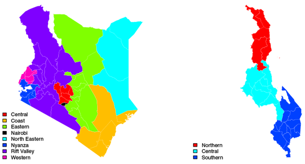
Administrative areas in Kenya (left) and Malawi (right). Colors show the eight Admin-1 areas of Kenya and the three Admin-1 areas of Malawi. The white borders outline the 47 Admin-2 areas of Kenya and the 28 Admin-2 areas of Malawi

2 |. DATA

To construct estimates of U5MR for Admin-2 areas over the period 1980 to 2014 for Kenya and 1980 to 2015 for Malawi, we make use of DHS survey data, MICS survey data and census data. Table 1 breaks down the data sources by type for each country. The FBH data come from either DHS surveys or MICS surveys, which have a stratified two-stage cluster design. Sampling frames are constructed from the most recent census, and consist of collections of households, labeled as enumeration areas (EAs) or clusters. Each of these clusters is classified as either urban or rural, as defined by each country (and these definitions can change over time, as new censuses are performed). Depending on the total number of clusters to be sampled, the strata consist of some administrative level (usually Admin-1) crossed with urban/rural. After this stratification, two-stage cluster sampling is performed selecting first EAs within strata and then households within EAs.^7–13 All women aged 15 to 49 who slept in a selected household the night before are eligible to be interviewed. In all DHS, and recent MICS, mothers are asked for the birth and death dates of all of their children in addition to many other questions. In certain older MICS and in censuses, only SBH data are collected. Full census data does not typically contain subnational geographic information, so we use 10% census samples with geographical information, as published by IPUMS-International.¹⁴ As Table 1 shows, in time periods where IPUMS census samples are available, they comprise an overwhelming proportion of births. Although they do not provide birth and death dates, which drastically reduces the effective amount of information.

TABLE 1.

List of all data sources and types for Kenya and Malawi. Columns 6-12 show the percentage of births each data source contributes to each five-year period

					Percentage births by period
Country	Source	Type	Year	Coverage	80–84	85-89	90-94	95-99	00-04	05-09	10-14
Kenya	DHS	FBH	2003	Nationala	0.5	36.5	0.7	21.1	0.4	0.0	0.0
			2008	National	0.2	21.1	0.5	17.1	0.4	16.3	0.0
			2014	National	0.0	26.9	1.0	42.2	1.2	62.0	78.3
	MICS	SBH	2000	Nationala	0.0	0.0	2.1	3.8	0.0	0.0	0.0
		FBH	2011	1 Admin-1	0.0	12.2	0.3	11.0	0.3	14.4	12.9
			2013	3 Admin-2	0.0	3.3	0.1	4.8	0.1	7.3	8.9
	IPUMS	SBH	1989	National	99.3	0.0	0.0	0.0	0.0	0.0	0.0
			1999	National	0.0	0.0	95.3	0.0	0.0	0.0	0.0
			2009	National	0.0	0.0	0.0	0.0	97.7	0.0	0.0
Malawi	DHS	FBH	2000	National	1.1	25.8	1.9	17.1	1.1	0.0	0.0
			2004	National	0.6	15.8	1.3	13.0	1.7	0.0	0.0
			2010	National	0.4	17.1	1.6	18.0	2.8	27.5	23.1
			2015	National	0.0	5.5	0.8	11.7	2.1	23.1	38.3
	MICS	FBH	2006	National	0.9	26.9	2.4	25.9	3.8	23.5	0.0
			2014	National	0.0	8.8	1.1	14.3	2.4	25.9	38.6
	IPUMS	SBH	1987	National	96.8	0.0	0.0	0.0	0.0	0.0	0.0
			1998	National	0.0	0.0	91.0	0.0	0.0	0.0	0.0
			2008	National	0.0	0.0	0.0	0.0	86.1	0.0	0.0

^aThis survey was carried out nationally, but does not have observations in all Admin-2 areas.

3 |. METHODS

Even when considering both household survey and census data, the amount of information is sparse in some cells defined by Admin-2 areas and years. We are in a classic small area estimation (SAE) context and, in general, when one analyzes survey data with a complex design one may follow design-based or model-based approaches. The former leans on traditional survey sampling techniques based on weighted estimates while the latter models the outcome (a count in our case) directly, and attempts to include terms in the model to account for the design. In either case, the sparsity of data across time and space leads to the necessity of using spatiotemporal smoothing models to borrow information.

The approach we take for smoothing is an extension of the famous Fay-Herriot¹⁵ model in which, in each time period and area, the observed data are summarized via a weighted estimate and its associated variance. These estimates are then modeled within a hierarchical framework, which we describe in this section. We refer to the overall method as smoothed direct since it takes the direct estimates (SAE terminology for estimates based on response data only from the area/time period for which estimates are required) and then smooths them across space and time. Among SAE models, an important distinction is between area-level models, such as the Fay-Herriot model, and unit-level models.¹⁶ We adopt area-level models in this paper, though in other work¹⁷ we use unit-level models, with the units corresponding to the sampled clusters in the FBH data. Currently, it is more difficult to use unit-level models when FBH and SBH data are combined.

The information in the FBH data allow the fitting of a discrete survival model, in order to estimate the U5MR. However, sparsity of data means that the data often require aggregating over multiple years, in order to obtain point and variance estimates. Specialized methods are required to exploit the limited information in the SBH data, but to use the smoothed direct method, all that is required is a point estimate and variance, and here we utilize the Brass method¹⁸ which provides an estimate (and SE) of U5MR in a particular year. In Section 3.1 we will review the method that we have previously used for making smoothed Admin-1 estimates of U5MR from DHS FBH data.^5,6 Section 3.2 then provides a review of the Brass method that we will use to analyze SBH data. In Section 3.3 we describe the latent temporal model that allows combination of 1-year and 5-year estimates. Next, Section 3.4 outlines the adjustment required for areas with small sample sizes.

3.1 |. Review of smoothed direct estimation

FBH data are collected via household surveys with stratified, multistage cluster sampling designs. To estimate the U5MR in a particular area and time, we fit a discrete hazards model. Using a weighted likelihood we account for the sampling scheme in our analysis. The birth dates and age at death are collected to the nearest month, or imputed where needed. Within the first 5 years of life, the hazard function varies greatly. In particular, deaths in the first month of life (neonatal deaths) were estimated to account for 47% of all under five deaths worldwide, in 2018.¹⁹ Due to the rapidly changing hazard function over ages 0 to 60 months, we follow the majority of previous approaches and adopt a discrete hazards model, on a monthly age scale.^6,20–23

To this end, we begin by expanding a child’s reported birth date and death date into months, where the response in each month is whether the child died or not. Using traditional demographic notation, we let

$${}_n{q}_x=\mathrm{Pr}(\mathrm{death\; before\; age}x+n|\mathrm{survival\; until\; age}x),$$

where x and n are in months. Thus, the probability of death before a child’s fifth birthday (60th month of life), is denoted ₆₀q₀. Following previous work,^5,6 we do not have a distinct discrete hazard for each of the 60 months, but rather we assume that the hazard is constant within each of six age-bands indexed by a = 1, 2, … ,6, and corresponding to months in the intervals [0, 1), [1, 12), [12, 24), [24, 36), [36, 48), [48, 60). This allows the model the flexibility to be able to make estimates for other important demographic measures such as the neonatal mortality rate, ₁q₀, and the infant mortality rate, ₁₁q₁. Note that, to be consistent with the literature we are referring to rates (including the U5MR) but we are actually modeling probabilities of death. It turns out that, in spite of the dependent observations on each child, the hazards can be estimated using a binomial likelihood with a logistic regression model.²⁴ Specifically, if we consider areas i = 1, … , n, time periods t = 1, … , T and data source s = 1 … , S, we have,

$$\mathrm{logit}({}_1{q}_{x,its})={\beta }_{a[x],its,}$$ (1)

where a[x] is a function that maps monthly age x to one of our six age bands a = 1, … ,6 and ₁q_x,its is the probability of death within 1 month given survival to age x for a child in area i and time t from data source s. To account for the complex design by which the data are collected, a pseudolikelihood method²⁵ is used to estimate the coefficients in (1). The method uses the survey weights provided by the DHS, which account for each child’s probability of being sampled and adjust for nonresponse, to weight each observation’s contribution to the score function that is used to estimate the hazards. This approach yields design-consistent estimates of the monthly hazard for each age band along with the estimated 6 × 6 variance-covariance of the estimates, ${\widehat{\Sigma }}_{its}$ using a sandwich estimator.²⁵ The model is fitted in R using the survey package.²⁶

We model the logit of the weighted estimate of the U5MR. From the estimates ${\widehat{\beta }}_{a[x],its}$, one can derive an estimate of ₆₀q_0,its,

$${}_{60}{\widehat{q}}_{0,its}=1-\prod _a{(1-{}_1{\widehat{q}}_{a[x],its})}^{n[a]},$$

where n[a] = 1, 11, 12, 12, 12, 12 for a = 1, 2, 3, 4, 5, 6, corresponding to the number of months in each of the six previously defined age intervals. The key idea in the Fay-Herriott approach is to take as observed data the weighted estimate (or some function of it) and then smooth. We let

$$y_{its}=\mathrm{logit}({}_{60}{\widehat{q}}_{0,its}).$$

The design-based variance of the estimator, ${\widehat{V}}_{its}$, can be obtained using the delta method and based on ${\widehat{\Sigma }}_{its}$, details are available in the supplementary materials of Mercer et al.⁵ Our hierarchical smoothing model begins with a likelihood which is taken as the asymptotic distribution of the estimator,

$$y_{its}|{\eta }_{its}\sim \text{N}({\eta }_{its},{\widehat{V}}_{its}).$$ (2)

We then decompose the logit of the true (unobserved) probability as,

$${\eta }_{its}=\mu +{\alpha }_t+{\gamma }_t+{\theta }_i+{\varphi }_i+{\delta }_{it}+v_s,$$ (3)

where μ is the overall mean, and the remainder of the terms smooth to either locally (dependent terms) or globally (independent terms) in space, time, or both. The terms ${\nu }_s\sim {}_{\mathrm{IID}}\text{N}\left(0,{\kappa }_{\nu }^{-1}\right)$, where IID is short hand for independent and identically distributed, estimate the bias of estimates from data source s, relative to μ. Together, γ_t and α_t comprise the temporal components of the model. Random “shocks” in time are modeled with ${\alpha }_t\sim {}_{\mathrm{IID}}\text{N}\left(0,{\kappa }_{\alpha }^{-1}\right)$. The smooth temporal trend is modeled by assigning γ_t, a random walk of order 2 (RW2). This model is defined by placing a prior on second differences,

$$\pi (\mathit{\gamma }|{\kappa }_{\gamma })\propto {\kappa }_{\gamma }^{(T-2)/2}\exp \left[-\frac{{\kappa }_{\gamma }}{2}\sum _{t=1}^{T-2}{({\gamma }_t-2{\gamma }_{t+1}+{\gamma }_{t+2})}^2\right]={\kappa }_{\gamma }^{(T-2)/2}\exp \left[-\frac{{\kappa }_{\gamma }}{2}{\mathit{\gamma }}^{\text{T}}{\mathbf{Q}}_{\gamma }\mathit{\gamma }\right],$$

where Q_γ specifies the second order dependency between time points and has rank T – 2, so that the prior is improper.²⁷ Following Besag, York and Mollié²⁸ (BYM), ${\varphi }_i\sim {}_{\mathrm{IID}}\text{N}(0,{\kappa }_{\varphi }^{-1})$, and θ_i is an intrinsic conditional autoregressive (ICAR) spatial random effect. The improper prior for θ_i encourages the borrowing of information from area i’s neighbors, which we define as those areas that share a common boundary,

$${\theta }_i|{\theta }_j,j\sim i,{\kappa }_{\theta }\sim \text{N}\left(\frac{1}{n_i}\sum _{j\sim i}{\theta }_j,\frac{1}{n_i{\kappa }_{\theta }}\right),$$

where j~i indexes the neighbors of area i and n_i are the number of such neighbors. The joint “distribution” is compactly written as

$$\pi (\mathit{\theta }|{\kappa }_{\theta })\propto {\kappa }_{\theta }^{(n-1)/2}\exp \left[-\frac{{\kappa }_{\theta }}{2}{\mathit{\theta }}^{\text{T}}{\mathbf{Q}}_{\theta }\mathit{\theta }\right],$$

where Q_θ encodes the neighbors. Finally, the space-time interaction, δ_it, is a Type IV interaction as defined by Knorr-Held.²⁹ This model accounts for contributions to the fit beyond the main effects by assuming the interactions have temporal and spatial structure. Specifically, the precision matrix is the kronecker product of the precision matrices of a RW2 and an ICAR, that is, Q_δ = Q_γ ⊗ Q_θ. We can write the joint “distribution” as,

$$\pi (\mathit{\delta }|{\kappa }_{\delta })\propto {\kappa }_{\delta }^{(n-1)(T-2)/2}\exp \left[-\frac{{\kappa }_{\delta }}{2}{\mathit{\delta }}^{\text{T}}{\mathbf{Q}}_{\delta }\mathit{\delta }\right].$$

This form is improper, since the matrix Q_δ has rank (n − 1)(T − 2). The final stage of the model is to specify priors on the intercept μ and the precisions κ_ν, κ_α, κ_γ, κ_θ, κ_ϕ, κ_δ. We use a normal prior with a large variance on the intercept, and penalized complexity priors on the precisions.³⁰

Specifically, PC priors penalize deviations from a null (fixed effects model). The priors are applied independently for ${\alpha }_t,{\gamma }_t,{\theta }_i^{\star }+{\varphi }_i^{\star }$ and δ_it. We adopt the BYM2 prior of Riebler et al,³¹ which places a joint PC prior on the structured spatial term, ${\theta }_i^{\star }$, and the unstructured spatial term, ${\varphi }_i^{\star }$. The prior on the spatial terms has two parameters, one which represents the proportion of the marginal variance, r_BYM, which is attributed to the ICAR term instead of the IID term and one which represents the marginal precision, κ_BYM, of the weighted sum of θ_i and ϕ_i. In the resulting linear predictor,

$${\theta }_i^{\star }+{\varphi }_i^{\star }={\kappa }_{\mathrm{BYM}}^{-1/2}\left[\sqrt{r_{\mathrm{BYM}}}{\theta }_i+\sqrt{1-r_{\mathrm{BYM}}}{\varphi }_i\right].$$

The model is fit via integrated nested Laplace approximation (INLA) using the R–INLA package,^32,33 which is very fast. After fitting the model, one obtains smoothed direct estimates and credible intervals via the posterior distribution for

$${}_{60}{q}_{0,its}=\mathrm{expit}(\mu +{\alpha }_t+{\gamma }_t+{\theta }_i+{\varphi }_i+{\delta }_{it}),$$

where we note that the study specific random effects ν_s terms are not included. The complete distributions are available, but we can summarize using, for example, the 5%, 50% and 95% quantiles.

3.2 |. Brass method

Censuses and some household surveys such as MICS provide SBH data: the age of the mother, the number of children ever born and the number of children ever died. We would like to include such data in analyses, but to use the method described in the previous section we require a point estimate, along with a standard error. A number of different methods have been described to analyze summary birth history data.^18,34–38 We describe and use the Brass method as it is the most commonly used method to analyze SBH data,^39,40 and has the most straightforward implementation. None of the other methods have an available implementation in the R programming environment. The Brass method is available in the SUMMER R package.⁴¹ The original method used the proportion of children ever died to children ever born in 5-year age groups of mothers to make an estimate of ₆₀q₀, the U5MR.¹⁸ Specifically, mothers ages are broken down into 5-year bands, 15 – 19, … ,45 – 49. The proportion of children who have died to mothers in age group a, d_a, is first calculated. This proportion is a function of the underlying probabilities of giving birth at different ages and the child mortalities by age of the population over the relevant time period. Brass equated these proportions of dead children to different mortalities depending on the associated age group. For example (see p228 of Preston et al⁴⁰), the proportion dead born to the 15 to 19 group corresponds to death within the first year of life, the 20 to 24 group to death in the first 2 years of life, and the 30 to 34 age group corresponds to death in the first 5 years (the U5MR). For the age groups that do not directly equate to U5MR (ie, all but the 30- to 34-year age group), a life table can be leveraged to convert to U5MR. Extensions have been made to account for parity of women by age groups in the sample and to attach a reference date of the estimate, a year in time prior to the census or survey.^42,43

More formally, suppose d_a is the probability of death in mother’s age a. This proportion approximates death before age x for some age x that depends on a. This basic relationship will change as a function of the reproductive histories of the women who supplied the data. Details on these histories are unavailable, and instead information on the parities in the relevant population are used in an empirical model that adjusts the mortality estimate. Specifically, for each age group, the following adjustment is used,

$${}_x{q}_0=d_a\left(b_{1a}+b_{2a}\frac{P_1}{P_2}+b_{3a}\frac{P_2}{P_3}\right),$$

where P₁, P₂, P₃ are average parities of mothers in age groups 15 to 19, 20 to 24 and 25 to 29, respectively, that provide some empirical estimates of birth timing. The coefficients b_1a, b_2a, b_3a were estimated via simulation using model life tables for fertility and mortality schedules.^42,44 Different coefficients are used in different settings, and we use the Coale and Demeny⁴⁵ (C-D) North life table coefficients in our analysis, which is the version that is relevant for Kenya and Malawi. These coefficients are available in table 47 of Hill et al.³⁹

The final step is to assign the estimate to a relevant period in the past, and another set of simulated coefficients, c_1a, c_2a, c_3a, are used in conjunction with the parity ratios to estimate a reference date,⁴³

$$c_{1a}+c_{2a}\frac{P_1}{P_2}+c_{3a}\frac{P_2}{P_3}.$$

As already discussed, the age group 30 to 34 directly produces an estimate of ₆₀q₀. Additionally, there is bias associated with SBH data from younger mothers, as they have a higher proportion of first births and first births have higher mortality rates.⁴⁶ For these reasons we use U5MR estimates from women aged 30–34 only.

Our smoothing model requires a point estimate and a variance estimate, but traditional Brass methods and variants do not provide uncertainty estimates. We use a jackknife to estimate ${\widehat{V}}_{its}$ for SBH data.²⁰ For the MICS surveys that provide SBH data, we must acknowledge the complex design, and we use a stratified cluster jackknife that removes clusters within strata. Let $y^{\left(hc\right)}=\mathrm{logit}({}_{60}\widehat{q}{}_{0,its}^{\left(hc\right)})$ be the estimate computed via the Brass method when the data from cluster c in strata h are removed for h = 1, … , H strata, with $c=1,\dots ,n_{its}^{(h)}$ clusters in area i, at time t in strata h for study s. The estimate of the logit of U5MR for strata h, for i, t, s, is,

$$y_{its}^{(h)}=\frac{1}{n_{its}^{(h)}}\sum _{c=1}^{n_{its}^{(h)}}{y}_{its}^{(hc)},$$

where $y_{its}^{(hc)}$ is the Brass estimate obtained when cluster c in strata h is removed. The stratified-cluster jackknife variance is,

$${\widehat{V}}_{its}=\sum _{h=1}^H\frac{n_{its}^{(h)}-1}{n_{its}^{(h)}}\sum _{c=1}^{n_{its}^{(h)}}{(y_{its}^{(hc)}-y_{its}^{(h)})}^2.$$

As each cluster-wise deletion must result in an estimate $y_{its}^{(hc)}$, we cannot calculate a measure of uncertainty for area, time, study combinations in which there are less than two clusters in each strata. Moreover, if deleting a cluster c within a strata h results in the observed proportion of deaths being zero, then $y_{its}^{(hc)}$ is undefined and we cannot compute the jackknife estimate of the variance for that area, time, study combination.

For the census samples we use a jackknife that removes women, as there are no design complications. There are, however, a large number of women in any given census and so we delete groups of women.²⁰ First, we select the size of groups to delete as d = 30. Then, for each census we calculate the number of groups as n_d = N/d (in practice we round), where N is the number of women in the IPUMS census sample. Let $y_{its}^{\left(k\right)}=\mathrm{logit}({}_{60}\widehat{q}{}_{0,its}^{\left(k\right)})$ denote the estimate computed via the Brass method when data from women in group k are removed. Then,

$${\widehat{V}}_{its}=\frac{n_d-1}{n_d}\sum _{k=1}^{n_d}{(y_{its}^{\left(k\right)}-y_{its})}^2,$$

where $y_{its}=\frac{1}{n_d}{\sum }_{k=1}^{n_d}{y}_{its}^{\left(k\right)}$

3.3 |. Latent temporal modeling

Both the FBH and SBH data produce a data pair [$\mathrm{logit}\left({}_{60}\widehat{q}{}_{0,its}\right),{\widehat{V}}_{its}$], that is, a point estimate and a variance, upon which a normal likelihood can be based. For the FBH data t refers to a five-year period, with t = 1980 to 1984, …, 2010 to 2014. For the SBH data, t refers to a single year (the reference year) between 1980 and 2014. To incorporate both 1-year and 5-year estimates in the direct smoothing model⁵ we specify all time-related random effects on the yearly scale, which means that we have to aggregate over 5-year periods for the FBH data. Recall the model defined by (2) and (3) includes a RW2, IID effects for each period and a Type-IV interaction term for all area and time period combinations. We reformulate the model for each of these effects.

We still include a RW2 term, γ_t, but the random walk is defined on the yearly scale and effects for periods are averages of the yearly effects within that period. Let t = 1, … , n_T index 1-year time points, t^⋆ = 1, … , n_T^⋆ index 5-year periods. We then collect together the smoothing random effects on the 1-yearly and 5-yearly scales as $\mathit{\gamma }={\left[{\mathit{\gamma }}_{\text{T}}^{\text{T}}{\mathit{\gamma }}_{{\text{T}}^{\star }}^{\text{T}}\right]}^{\text{T}}$ where γ_Tis a vector of length n_T and γ_T⋆ is a vector of length n_T^⋆. We define

$${\mathit{\gamma }}_{\text{T}\star }=\mathbf{A}{\mathit{\gamma }}_{\text{T}},$$ (4)

where A is an n_T^* × n_T matrix that averages each consecutive set of n_T/n_T^⋆ points. The coarsened parameters γ_T⋆ are a deterministic function of the yearly versions γ_T but both are needed to define the model, for the FBH and SBH data, respectively. In our case, n_T = 35 and n_T^⋆ = 7, so that γ_T^⋆ is a 7 × 1 vector of five-year averages. The RW2(κ_γ) prior on γ_T can be written

$$\pi ({\mathit{\gamma }}_{\text{T}}|{\kappa }_{\gamma })\propto {\kappa }_{\gamma }^{(n_{\text{T}}-2)/2}\exp \left[-\frac{{\kappa }_{\gamma }}{2}{\mathit{\gamma }}_{\text{T}}^{\text{T}}{\mathbf{Q}}_{\gamma }{\mathit{\gamma }}_{\text{T}}\right],$$

where κ_γ Q_γ is the precision matrix of the random walk. We practically implement the relationship (4) in INLA via a soft constraint in which we assume ${\mathit{\gamma }}_{{\text{T}}^{\star }}|{\mathit{\gamma }}_{\text{T}}\sim \text{N}(\mathbf{A}{\mathit{\gamma }}_{\text{T}},{\tau }_{\gamma }^{-1}{I}_{n_{{\text{T}}^{\star }}}^{-1})$, where I_nT^⋆ is the identity matrix and τ_γ = 10⁶. Written out in full,

$$\pi ({\mathit{\gamma }}_{{\text{T}}^{\star }}|{\mathit{\gamma }}_{\text{T}})\propto {\tau }_{\gamma }^{n_{{\text{T}}^{\star }}/2}\exp \left[-\frac{{\tau }_{\gamma }}{2}{({\mathit{\gamma }}_{{\text{T}}^{\star }}-\mathbf{A}\mathit{\gamma }\text{T})}^{\text{T}}{\mathbf{I}}_{n_{{\text{T}}^{\star }}}({\mathit{\gamma }}_{{\text{T}}^{\star }}-\mathbf{A}{\mathit{\gamma }}_{\text{T}})\right].$$ (5)

Then, the joint prior on γ can be expressed as,

$$\pi (\mathit{\gamma })=\pi ({\mathit{\gamma }}_{\text{T}})\pi ({\mathit{\gamma }}_{\text{T}\star }|{\mathit{\gamma }}_t)\propto \exp \left[-\frac{1}{2}{\mathit{\gamma }}^{\text{T}}{\mathbf{Q}}_{\gamma }^{†}\mathit{\gamma }\right],$$

where

$${\mathbf{Q}}_{\gamma }^{†}=\left[\begin{array}{cc}{\kappa }_{\gamma }{\mathbf{Q}}_{\gamma }+{\tau }_{\gamma }{\mathbf{A}}^{\text{T}}\mathbf{A}& -{\tau }_{\gamma }{\mathbf{A}}^{\text{T}}\\ -{\tau }_{\gamma }\mathbf{A}& {\tau }_{\gamma }{\mathbf{I}}_{n_{{\text{T}}^{\star }}}\end{array}\right].$$

We can define the IID model similarly, where $\mathit{\alpha }={[\begin{array}{cc}{\mathit{\alpha }}_{n_{\text{T}}}^{\text{T}}& {\mathit{\alpha }}_{n_{\text{T}}{}^{\star }}^{\text{T}}\end{array}]}^{\text{T}}$ is the stacked vector of yearly IID effects and period IID effects and

$$\pi ({\mathit{\alpha }}_{n_{\text{T}}})={(2\pi )}^{-n_{n_{\text{T}}}/2}{\kappa }_{\alpha }^{n_{n_{\text{T}}}/2}\exp \left[-\frac{{\kappa }_{\mathit{\alpha }}}{2}{\mathit{\alpha }}_{n_{\text{T}}}^{\text{T}}{\mathbf{I}}_{n_{\text{T}}}{\mathit{\alpha }}_{n_{\text{T}}}\right].$$

Then, π(α_T^⋆ | α_T) is defined analogously to (5), and

$$\pi (\mathit{\alpha })=\pi ({\mathit{\alpha }}_{\text{T}})\pi ({\mathit{\alpha }}_{{\text{T}}^{\star }}|{\mathit{\alpha }}_{\text{T}})\propto \exp \left[-\frac{1}{2}{\mathit{\alpha }}^{\text{T}}{\mathbf{Q}}_{\alpha }^{†}\mathit{\alpha }\right],$$

where

$${\mathbf{Q}}_{\alpha }^{†}=\left[\begin{array}{cc}{\kappa }_{\alpha }{\mathbf{I}}_{n_{\text{T}}}+{\tau }_{\alpha }{\mathbf{A}}^{\text{T}}\mathbf{A}& -{\tau }_{\alpha }{\mathbf{A}}^{\text{T}}\\ -{\tau }_{\alpha }\mathbf{A}& {\tau }_{\alpha }{\mathbf{I}}_{n_{{\text{T}}^{\star }}}\end{array}\right].$$

We again define a space-time interaction model using a Type IV interaction as described by Knorr-Held.²⁹ To specify the prior for all space-time interactions, first define $\mathit{\delta }={[\begin{array}{cc}{\mathit{\delta }}_{\text{T}}^{\text{T}}& {\mathit{\delta }}_{{\text{T}}^{\star }}^{\text{T}}\end{array}]}^{\text{T}}$ where δ_T is the (n × n_T) × 1 vector of yearly interactions, and δ_T^⋆ is the (n × n_T^⋆) × 1 vector of interactions defined with respect to periods, and n is the number of areas. Then,

$$\pi ({\mathit{\delta }}_{\text{T}})\propto \exp \left[-\frac{\kappa \delta }{2}{\mathit{\delta }}_{\text{T}}^{\text{T}}{\mathbf{Q}}_{\delta }{\mathit{\delta }}_{\text{T}}\right],$$

where the dependency structure is defined as Q_δ = Q_γ ⊗ Q_θ and Q_γ and Q_θ specify the dependency structures of the RW2 and ICAR models, respectively. Then δ_T^⋆ = Bδ_T, where B is an (n × n_T^⋆) × (n × n_T) matrix that consists of n copies of A on the diagonal and zeroes elsewhere. Then,

$$\pi (\mathit{\delta })=\pi ({\mathit{\delta }}_{\text{T}})\pi ({\mathit{\delta }}_{{\text{T}}^{\star }}|{\mathit{\delta }}_{\text{T}})\propto \exp \left[-\frac{1}{2}{\mathit{\delta }}^{\text{T}}{\mathbf{Q}}_{\delta }^{†}\mathit{\delta }\right],$$

where

$${\mathbf{Q}}_{\delta }^{†}=\left[\begin{array}{cc}{\kappa }_{\delta }{\mathbf{Q}}_{\delta }+{\tau }_{\delta }{\mathbf{B}}^{\text{T}}\mathbf{B}& -{\tau }_{\delta }{\mathbf{B}}^{\text{T}}\\ -{\tau }_{\delta }\mathbf{B}& {\tau }_{\delta }{\mathbf{I}}_{{n\times n}_{{\text{T}}^{\star }}}\end{array}\right].$$

These specifications of the time effects allow us to smooth in time and incorporate data on both yearly and period scales. This also allows us to easily make estimates and predictions on both yearly and period scales.

3.4 |. Zero adjustment

Most household surveys are geographically stratified at an administration level higher than Admin-2, thus sample sizes can be small or nonexistent in some Admin-2 areas. If the data are sparse, we may not observe any deaths in such an area, leading to a direct estimate of ${}_{60}{\widehat{q}}_{0,its}=0$. In these cases, and in cases where all the children in a cluster have the same response (all deaths or all nondeaths), the variance estimate is 0. These cases are problematic for our smoothing model as $\mathrm{logit}({}_{60}{\widehat{q}}_{0,its})$ is undefined and we require a (nonzero) design-based variance. In the case of no data in an area and time period, we treat these as missing values, which can be dealt with accordingly within a Bayesian framework. In the aforementioned other cases, we cannot go this route, as they are informative, albeit weakly.

We propose a model-based solution for areas where we have computational issues; we preprocess such data to replace the problematic estimates with a reasonable value. We stress that this should only be carried out for a small proportion of areas and time periods. In a problematic area labeled i, we take the set of its first order neighbors j ~ i, to constitute a larger area. For the problematic areas and its neighbors we fit a betabinomial model that accounts for the complex survey design by including an urban/rural strata fixed effect and a scale parameter that allows for clustering. We let i index areas, h strata, and c clusters within strata. For a time period t and a survey s,

$$Z_{its}^{(hc)}|{{}_{60}q}_{0,its}^{\left(\mathit{hc}\right)}\sim \mathrm{BetaBinomial}(n_{its}^{(hc)},{{}_{60}q}_{0,its}^{\left(\mathit{hc}\right)},d),$$

$$\mathrm{logit}({{}_{60}q}_{0,its}^{\left(\mathit{hc}\right)})=\mu +\beta 1(h=2)+e_i,$$

$$e_i\sim \text{N}(0,{\sigma }_e^2),$$

where $Z_{its}^{(hc)}$ is the number of deaths, $n_{its}^{(hc)}$ is the number of children in cluster c for urban and rural strata, h = 1, 2, and d is an overdispersion parameter. This model can be fitted in R with INLA; we use relatively uninformative priors on β, ${\sigma }_e^2$ and d.

An estimate of the aggregate U5MR in area i, time period t and for source s is,

$${}_{60}{q}_{0,its}=p_{its}\times \mathrm{expit}(\mu +e_i)+(1-p_{its})\times \mathrm{expit}(\mu +\beta +e_i),$$ (6)

where p_its and 1 – p_its are the proportions of births that are urban and rural, respectively. In the DHS sampling manuals, the numbers of clusters in urban and rural strata in the sampling frame is reported by area—usually this is by Admin-1, but it is Admin-2 for some surveys, including the ones we use in Kenya and Malawi.

Within the INLA implementation in R there is a function inla.posterior.marginal, that allows one to draw samples [${\mu }^{\left(j\right)},{\beta }_h^{\left(j\right)},e_i^{\left(j\right)}$] for j = 1, … , J, from the approximate joint posterior distribution. These can be converted to samples ${}_{60}q{}_{0_{its}}^{\left(j\right)}$ using (6) and we use the posterior mean and posterior variance of these samples for y_its and ${\widehat{V}}_{its}$, respectively that we require for the smoothing model. Let $y_{its}^{\left(j\right)}=\mathrm{logit}({}_{60}q{}_{0,its}^{\left(j\right)})$, then

$$y_{its}=\frac{1}{J}\sum _{j=1}^J{y}_{its}^{(j)},$$

and

$${\widehat{V}}_{its}=\frac{1}{J-1}\sum _{j=1}^J{(y_{its}^{(j)}-y_{its})}^2.$$

We show results of the adjustment method for the 2003 Kenya DHS, as it has more areas and time periods that need to be adjusted. Malawi, on the other hand, has only a handful of areas/time periods that need adjustments, so results are relegated to Appendix. Figure 2 shows a side-by-side comparison of estimates of logit U5MR in all areas in Kenya before (Left) and after (Right) adjustment. Note, the estimates on the right-hand side and the corresponding variances used to create the confidence intervals are those later included in the smoothing model. Areas to be adjusted are in red in both panels. We see three types of estimates to be adjusted on the left. Lamu, Embu, Laikipia, Trans-Nzoia, Kajiado and Samburu all have an estimate of ${}_{60}{\widehat{q}}_{0,i,80-84,2003}=0$ and ${\widehat{V}}_{i,80-84,2003}=0$. Isiolo has no estimate, as no clusters in the 2003 DHS were sampled in that area. Lastly, Marsabit and West Pokot have ${}_{60}{\widehat{q}}_{0,i,80-84,2003}\ne 0$ and ${\widehat{V}}_{i,80-84,2003}=0$. In Marsabit there are four sampled households, in West Pokot there are five. In every household either all the children die or all the children survive, which leads to a variance estimate of 0. Figure A1 shows the location and types of adjustments on a map. Our adjusted estimates ${}_{60}{\widehat{q}}_{0,\mathrm{its}}$ are pulled away from 0 and informed by the data in surrounding areas. The average 95% CI width for adjusted areas is 2.01, which is nearly identical to the average width of unadjusted areas, 2.03.

FIGURE 2.

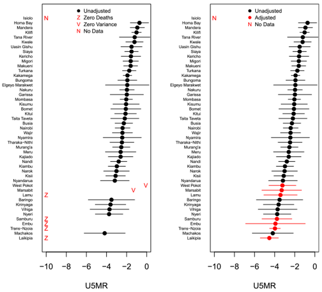
Left: The direct estimates on the logit scale for counties in Kenya from the 2003 DHS for 1980 to 1984. A red Z indicates an area with no observed deaths, whose logit U5MR is undefined. A red V indicates an area where deaths are observed, but estimated variances are zero. A red N indicates an area that contains no sampled clusters. Right: The adjustment comparisons on the logit scale

Figure 3 shows smoothed results on a map for the two ways of treating the observed zeroes for the period 1980 to 1984. Recall the pink areas, Marsabit and West Pokot, in Figure A1. These places had small sample sizes, with nonzero estimates of ${}_{60}{\widehat{q}}_{0,i,80-84,2003}$ and zero estimates of ${\widehat{V}}_{i,80-84,2003}$. In the left column of Figure 3, we see that when we throw out these observations, we get incredibly wide CIs. However, when we use the adjusted method we still estimate relatively high mortality, which we would expect since we observed deaths in this area, but our uncertainty decreases. In areas where we observe no deaths, we estimate smaller U5MRs when we use adjusted estimates instead of simply removing the data from the area. We also see shorter CI widths. Lastly, including the adjusted data allows us to make more precise estimates in Isiolo (outlined in navy) than when we throw out these Admin-2 area’s data. In Isiolo, we have no observations whatsoever from the 2003 DHS. However, the adjusted data from Isiolo’s neighbors that either had no observed deaths or an estimated variance of zero changes both the median estimate and the precision of the estimated U5MR in Isiolo after smoothing.

FIGURE 3.

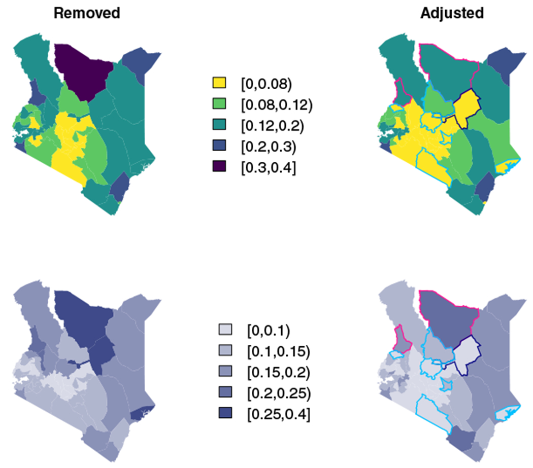
Top: Smoothed estimates for the period 1980 to 1984 when we throw out observed zeroes (Left) or adjust them (Right). Bottom: Width of 95% CI interval estimates for the period 1980 to 1984 when we throw out observed zeroes (Left) or adjust them (Right). Colored boundaries correspond to colors in Figure A1: pink are areas with observed deaths, but a zero variance estimate, light blue are areas with no observed deaths, and the navy outline is an area with no data

We end this section with a review of the literature that is relevant to the zero-adjustment procedure we have described. Some authors^47,48 have chosen to take as likelihood the sampling distribution of the estimator on the original scale (the U5MR in our setting) while smoothing on a different scale, in an approach labeled area-level unmatched sampling and linking models (the linking model is the second stage of the hierarchy, (3) in our case). This approach removes the numerical problems with the estimated probability being 0 or 1, though the asymptotic normal approximation to the sampling distribution is likely to be inaccurate in these cases. In Ha et al (section 3.2),⁴⁷ the design variance is written as the product of the variance of the estimator for a binomial response and the design effect. The former depends on the unknown proportion, and this is estimated using a synthetic estimator that uses data from a larger region, the design effect is also estimated from a larger region. Generalized variance function estimation (chapter 7 of Wolter⁴⁹) provides a general approach to alleviating problems of variance instability.

3.5 |. Space-time smoothing model

In this section we discuss two difficult practical issues. The first is that each data source has its own idiosyncrasies in design and data collection, which leads to a unique set of potential biases—estimates resulting from SBH data in particular may be subject to bias,³⁵ and we do not want them to have undue influence on our smoothed estimates. The second difficulty is that even though the IPUMS data are a 10% sample, the census data can dominate in terms of information available. The previous version of the model in Equations (2) and (3) had a normal likelihood, and a random effect for source type. We remove the latter term for the overall estimates, which is consistent with believing that the study types are exchangeable, and no more or less likely to be susceptible to bias. We now change this specification to have fixed effects associated with the SBH data, to allow for the possibility of bias. The inclusion of these bias correction terms corrects for a data source having consistently low or high estimates and these fixed effects are assumed constant across time and space. The new model is,

$$\mathrm{logit}({}_{60}{\widehat{q}}_{0,its})\sim \text{N}({\eta }_{its},{\widehat{V}}_{its}),$$ (7)

$${\eta }_{its}=\mu +{\beta }_s\mathbf{1}(s\text{ is SBH})+{\alpha }_t+{\gamma }_t+{\theta }_i^{\star }+{\varphi }_i^{\star }+{\delta }_{it},$$ (8)

where individual β_s are fixed bias correction terms for each data source s that provides SBH data. This allows these data sources to contribute to understanding temporal, spatial and spatiotemporal variability, but not the absolute level.

4 |. APPLICATION OF METHODS TO KENYA AND MALAWI MORTALITY DATA

We apply the methods detailed in Section 2 to the data found in Table 1. The Kenya DHS in 2014 and the Malawi DHS in both 2010 and 2015 were stratified at the Admin-2 level crossed with urban/rural, yielding sufficient sample sizes in all areas. However, the other DHS were stratified at the Admin-1 level. Figure 1 shows the difference in granularity of these administrative levels. Using jittered GPS locations of clusters sampled in the DHS stratified at the Admin-1 level, we can assign clusters to the appropriate Admin-2 area. For MICS surveys and IPUMS census samples, we do not have GPS locations, but we have place names. Usually, these place names are at an even finer granularity than Admin-2 (the census) or are no longer in use (older MICS and census). In these cases we query the Google Maps API to get a GPS location for the center associated with the name and then assign it to the appropriate Admin-2 area. Modeling at the subnational level also allows us to incorporate MICS surveys that were carried out with subnational coverage. In Kenya, this includes the 2011 MICS carried out in Nyanza (Admin-1) and three 2013 MICS carried out in Bungoma, Kakamega, and Turkana (Admin-2).

First, we process all data according to their type, using the survey-weighted discrete hazards survival method for the FBH data and the Brass method and jackknife for the SBH data. Then, we apply the adjustment for the areas that have no observed deaths or zero variance estimates. These areas account for 51 of the 987 DHS area, time, survey points (5.2%) in Kenya and just 14 of the 784 points (1.8%) in Malawi. There are no MICS FBH estimates that need adjustment. We next apply an adjustment to account for the generalized HIV/AIDS epidemic. The method developed by Walker et al⁵⁰ produces estimates of the proportion deaths of children born to women who have died due to HIV prior to a survey, HIV_its. The method takes as inputs the number of women of reproductive age, the number of HIV-positive women of reproductive age, the number of births and the HIV incidence in children. We take the latter information from Spectrum,⁵¹ a simulation software used to simulate the course of the HIV/AIDS epidemic in a country and calculates many demographic measures of the population. As survey data come from interviews with women aged 15 to 49, there is nonignorable missingness for mothers who have died from HIV, since the children of HIV-positive women are more likely to have died. To adjust our estimates, we divide by a correction factor

$${{}_{60}\widehat{q}}_{0,its}^{\mathrm{HIV}}=\frac{{{}_{60}\widehat{q}}_{0,its}}{1-{\mathrm{HIV}}_{its}},$$

with adjustments to ${\widehat{V}}_{its}$ being obtained via the delta method.

Once we have converted all of our data sources into [$\mathrm{logit}({{}_{60}\widehat{q}}_{0,its}^{\mathrm{HIV}})$, ${\widehat{V}}_{its}^{\mathrm{HIV}}$] pairs, we smooth these estimates across space and time using the model in (8) from Section 3.5. The posterior estimate of the SBH biases can be seen in Appendix D. To summarize, there is far more bias for the Kenya SBH data than for the Malawi data. To get estimates for an area i and time t, whether t is a year or a period, we take draws from the joint posterior. to compute ₆₀q_0,it. Fitting the model in INLA using 8GB for Malawi took 421 seconds with 28 Admin-2 areas. For Kenya’s 47 Admin-2 areas it took 1072 seconds, which is much longer but still a relatively short amount of time for such a complex Bayesian model.

4.1. Results

In this section we review results from the space-time smoothing model using the normal likelihood, (8). Figure 4 shows the data used in estimation and the smoothed estimates with 95% intervals for years 1980 to 2014 for two areas, Nairobi county in Kenya (Left) and Lilongwe district in Malawi (Right). Point sizes of the FBH and SBH estimates are weighted relative to the median 95% CI for any estimate in that Admin-2 area. Estimates from surveys and censuses with 95% CI widths larger than the median width in that Admin-2 area are shrunk at a ratio of the median width to the point’s CI. Points whose 95% CI widths are below the median width for that county are enlarged at a ratio of the median width to the point’s 95% CI width. Thus, larger points represent more precise estimates with narrower CIs and have a larger influence on the smoothing model than smaller points. In Nairobi, the increased mortality due to the HIV/AIDS epidemic is evident in the period between 1985 and 2005. Though U5MR in Nairobi has declined since the peak of the epidemic, its current U5MR is roughly the same as it was before the epidemic began. The additional information from the SBH estimates gives us a slightly different estimate of the time period of increased U5MR due to the HIV/AIDS crisis. Moreover, the rate at which U5MR has been declining in Nairobi has slowed in recent years. Addition of SBH data gives us shorter CI widths historically, and even slightly shorter PIs for the period 2015 to 2019. For Lilongwe, Figure 4 shows a large decline in child mortality over the period analyzed. The inclusion of SBH data provides us with expected precision gains, but only changes the U5MR trend in Lilongwe before 1990. Compared to Kenya, the Malawi SBH estimates are more consistent with the FBH estimates over time. Thus, in general, we see smaller differences in trends estimated with and without SBH data. Similar results for all Admin-2 areas in Malawi and Kenya can be found in Appendices G to J. National results for both Malawi and Kenya can be found in Appendix F.

FIGURE 4.

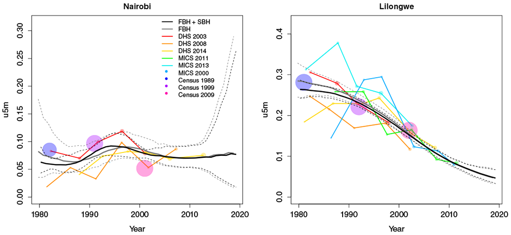
Survey and census estimates overlayed with smoothed estimates and intervals. Estimates connected by lines are direct estimates from either DHS or MICS; single points are Brass estimates from MICS or the census. For the estimates, the size of the point is weighted by the width of 95% CI. Larger points imply a shorter width and more precise estimates. Left: Results for Nairobi county in Kenya. Right: Results for Lilongwe district in Malawi

Figure 5 shows posterior median U5MR estimates in Malawi by district with and without SBH data for the period 2010 to 2014 on the top row. We see two Admin-2 areas in the Southern region (Neno and Mulanje) and one area in the Central region (Mchinji) with consistently high median estimates of U5MR regardless of the inclusion or exclusion of SBH data. Figure 6 shows the same set of results for Kenya. Three areas stand out as having particularly high U5MR relative to other Admin-2 areas: one in Rift Valley province (Turkana) and the other two in Nyanza province (Migori and Homa Bay). While both the minimum and maximum of the U5MR scale in Kenya is lower than in Malawi, the interval widths in Kenya tend to be larger. For both countries, the addition of SBH data leads to more Admin-2 areas with smaller 95% interval widths than estimates using only FBH data. This can be seen in the presence of more lightly shaded areas in the bottom right panels than in the bottom left panels of Figures 5 and 6.

FIGURE 5.

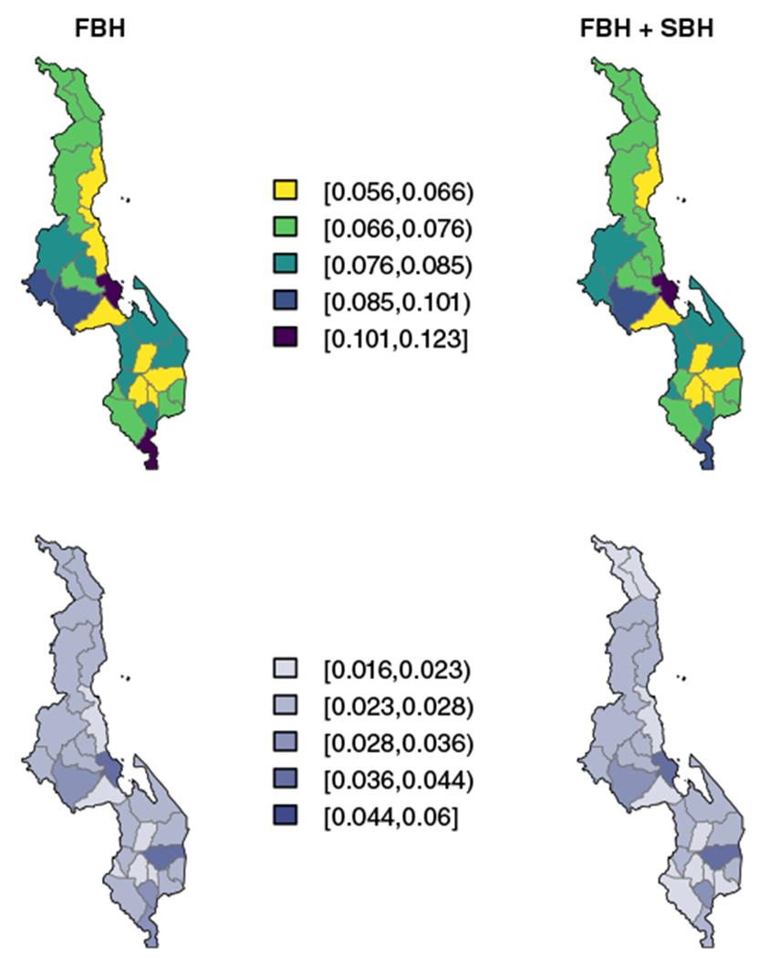
Results for Malawi by area for the period 2010 to 2014. Top: Smoothed estimates by area, with only full birth history (FBH) data (Equation (2)) (Left) and FBH and summary birth history (SBH) data (Right) (8). Bottom: 95% interval widths by area with FBH data only (Left) and FBH and SBH data (Right)

FIGURE 6.

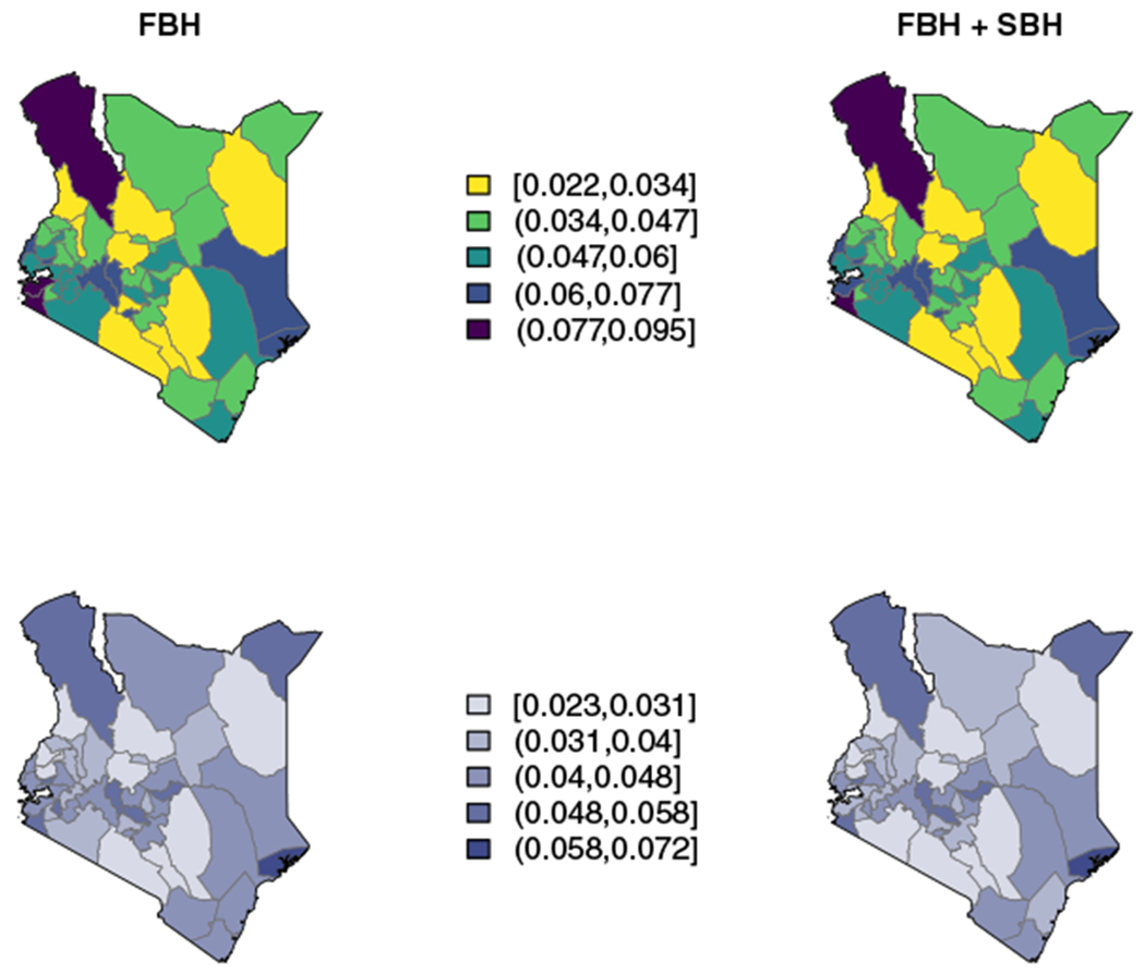
Results for Kenya by area for the period 2010 to 2014. Top: Smoothed estimates by area, with only full birth history (FBH) data (Equation (2)) (Left) and FBH and summary birth history (SBH) data (Right) (8). Bottom: 95% interval widths by area with FBH data only (Left) and FBH and SBH data (Right)

Figure 7 shows district-level estimates in 5-year periods from 1980-1984 to 2010-2014 and projections to 2015 to 2019 using all the data. The huge decline in U5MR over this period is easily seen. The relatively higher mortality of the Central region is also apparent relative to the Northern and Southern regions. Throughout the period of time analyzed, the Southern region appears to have more within region variability across Admin-2 areas than either the Northern or Central regions. Though there is still subnational variability in Malawi today, it is easier seen via the scale used in Figure 5 as all districts have relatively low U5MR compared to earlier periods. Relative subnational variation remains, however.

FIGURE 7.

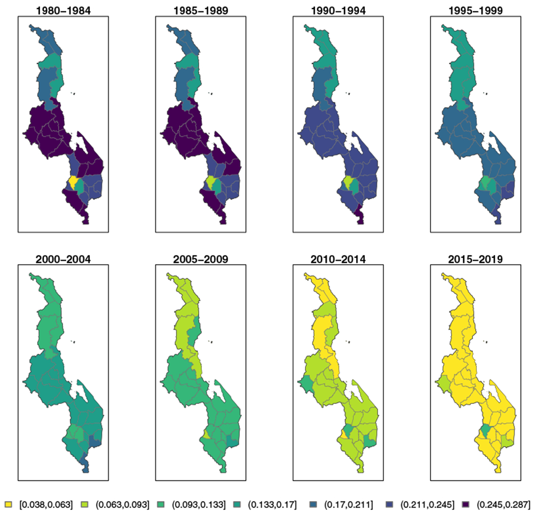
Median under-five mortality rate (U5MR) estimates for 5-year periods in districts in Malawi, using all data sources, from 1980-1984 to 2010-2014, with projections to 2015-2019

In Figure 8 we see a similar pattern of broad U5MR decline across all 47 counties in Kenya between the 1980-1984 and the 2010-2014 periods. However, the impact of the HIV/AIDS epidemic on U5MR in Kenya is apparent in the top row of Figure 8 as many areas underwent a clear rise in child mortality during this period, followed by a decline after the turn of the century. Consistently, counties in the Kenyan region of Nyanza experience higher relative mortality when compared to those in other regions. Though the highest experienced U5MRs in both Kenya and Malawi are similar, the lowest experienced and projected U5MRs in Kenya are a bit lower than in Malawi. Comparing the two figures, it is also evident that the high U5MR in the Nyanza region of Kenya lasted much later than in any region which previously experienced these high U5MRs in Malawi.

FIGURE 8.

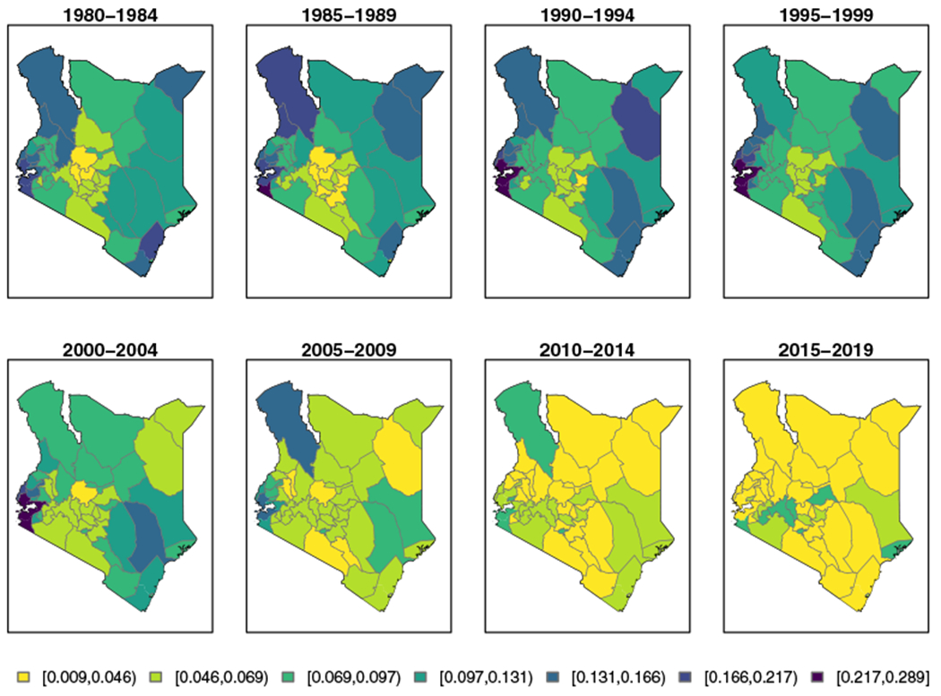
Median under-five mortality rate (U5MR) estimates for 5-year periods in counties in Kenya, using all data sources, from 1980-1984 to 2010-2014, with projections to 2015-2019

4.2 |. Validation

As an exercise in model validation, cycling through all areas and periods from 1990-1994 to 2010-2014, we leave out data from an area i and a time period t, fit our model and then make estimates of ₆₀q_0,it. We assess the performance by computing precision-weighted versions of standard model assessment statistics. Let ${\widehat{y}}_{it}$ be the smoothed median estimate of logit(₆₀q_0,it) and ${\widehat{V}}_{it}$ be its variance when data from area i and period t are omitted. We take

$${\widehat{y}}_{it}=\sum _{s\in F_{it}}{w}_{its}{\widehat{y}}_{its}=\sum _{s\in F_{it}}\frac{{\widehat{V}}_{its}^{-1}}{{\sum }_{s\in F_{it}}{\widehat{V}}_{its}^{-1}}{\widehat{y}}_{its},$$

and

$${\widehat{V}}_{it}=\frac{1}{{\sum }_{s\in F_{it}}{\widehat{V}}_{its}^{-1}},$$

where s ∈ F_it indicates s is an FBH data source for area i and time t, as measures of truth and variance, respectively, for each area and time period. Given that the estimates can have a wide range of precisions, we weight the estimate of the “truth” by its relative precision. For the MSE, then,

$${\mathrm{MSE}}_t=\sum _{i=1}^n{w}_{it}{(y_{it}-{\widehat{y}}_{it})}^2,$$

where n is the total number of areas and $w_{it}=\frac{{\widehat{V}}_{\mathit{it}}^{-1}}{\sum _{t=1}^I{\widehat{V}}_{\mathit{it}}^{-1}}$. Similarly, we can define the mean absolute error (MAE) as

$${\mathrm{MAE}}_t=\sum _{i=1}^n{w}_{it}|y_{it}-{\widehat{y}}_{it}|,$$

and the mean absolute percent error (MAPE) as,

$${\mathrm{MAPE}}_t=\sum _{i=1}^n{w}_{it}\frac{|{}_{60}{q}_{0,it}-{}_{60}{\widehat{q}}_{0,it}|}{{}_{60}{\widehat{q}}_{0,it}}$$

Tables 2 and 3 compare the above validation metrics between a model with only FBH data sources included and a model with both FBH and SBH data sources included. Reference dates for SBH estimates vary across space, but tend to contribute to a single 5-year period. For example, in Malawi, all Brass estimates from the 1987 census have reference dates between years 1980 and 1981, all estimates from the 1998 census lie between years 1991 and 1992, and all estimates from the 2008 census lie between years 2001 and 2002. This means the effect of incorporating SBH data into the model will have different effects in different time periods. As a result, we see that neither model out performs the other in all time periods. In all periods with SBH estimates, Table 2 shows the MSE is smaller for the model with both data types. For Kenya, we see the addition of SBH data decreases the MAE and MAPE for all periods with SBH data (1990-1994, 2000-2004) as well as in most other time periods. Comparing Appendices G to J shows much more between data source variability within Admin-2 area in Kenya than in Malawi. There is more estimated bias in the SBH data sources from Kenya than Malawi (see Figure D1). These factors all contribute to give larger estimates of validation metrics across the board in Kenya as compared to Malawi.

TABLE 2.

Assessment measures for Malawi by period comparing the full birth history (FBH) + summary birth history (SBH) smoothing model (columns 6-9) and the FBH smoothing model (columns 2-5) when leaving out data from each area and period. For each period, “best” values in each metric are bolded

	FBH				FBH + SBH
Year	Bias	MSE	MAE	MAPE	Bias	MSE	MAE	MAPE
1990-1994	0.001	0.030	0.107	0.096	0.003	0.024	0.089	0.078
1995-1999	0.001	0.041	0.108	0.083	−0.005	0.043	0.113	0.086
2000-2004	0.003	0.015	0.087	0.077	0.004	0.009	0.069	0.060
2005-2009	−0.009	0.022	0.122	0.100	−0.013	0.020	0.117	0.103
2010-2014	0.007	0.058	0.190	0.177	0.006	0.055	0.194	0.181
Mean	0.000	0.033	0.121	0.106	−0.001	0.030	0.116	0.102

TABLE 3.

Assessment measures for Kenya by period comparing the full birth history (FBH) + summary birth history (SBH)smoothing model (columns 6-9) and the FBH smoothing model (columns 2-5) when leaving out data from each area and period. For each period, “best” values in each metric are bolded

	FBH				FBH + SBH
Year	Bias	MSE	MAE	MAPE	Bias	MSE	MAE	MAPE
1990-1994	0.091	0.203	0.318	0.311	0.038	0.189	0.288	0.251
1995-1999	0.074	0.119	0.268	0.255	0.101	0.136	0.287	0.279
2000-2004	0.105	0.179	0.304	0.314	0.061	0.152	0.277	0.291
2005-2009	0.120	0.288	0.398	0.480	0.092	0.260	0.373	0.436
2010-2014	0.028	0.393	0.480	0.477	0.055	0.390	0.474	0.477
Mean	0.084	0.236	0.354	0.368	0.069	0.225	0.340	0.347

We perform an additional validation exercise by fitting the model to all data except the most recent DHS stratified at the Admin-2 level. Both the Kenya 2014 DHS and the Malawi 2015 DHS were stratified at a finer geographic level, and there are decent sample sizes in all areas and most time periods going back to 1985 to 1989. In this case, we use the direct estimate from these removed DHS surveys as the “truth” in our validation metrics. We calculate the same metrics as in the first validation exercise. In the scenario where we leave out the 2015 DHS in Malawi, the advantage to using both data sources is much clearer. Table 4 shows that in each of the six time periods assessed in this exercise, the MSE is much lower when we incorporate SBH data. In nearly all time periods the bias is also smaller with the incorporation of SBH data. In Kenya, Table 5 shows less evidence of improvements in estimates, but we do see decreases in MSE and MAPE in at least every time period with SBH data contributions. Moreover, the gains in MSE and MAPE tend to be larger in magnitude than in the cross-validation exercise. This is likely due to the fact that we remove much more data when moving an entire DHS survey (see Table 1) than when leaving out data for a single area and time period.

TABLE 4.

Assessment measures for Malawi by period comparing the full birth history (FBH) + summary birth history (SBH) smoothing model (columns 6-9) and the FBH smoothing model (columns 2-5) when leaving out the Malawi 2015 DHS and treating estimates from this survey as the “truth.” For each period, “best” values in each metric are bolded. (Note: results here exclude the district of Likoma. Removal of the 2015 DHS removes our only FBH data source with usable estimates for Likoma. Methods such as those included in Section 3.4 cannot be used as Likoma is an island, and is quite distinct from areas on the mainland, making a spatial smoothing model inappropriate.)

	FBH				FBH + SBH
Year	Bias	MSE	MAE	MAPE	Bias	MSE	MAE	MAPE
1985-1989	0.014	0.382	0.418	0.447	0.015	0.328	0.388	0.387
1990-1994	−0.310	0.202	0.390	0.273	−0.237	0.124	0.305	0.217
1995-1999	−0.353	0.234	0.431	0.308	−0.177	0.105	0.274	0.210
2000-2004	−0.370	0.237	0.427	0.302	−0.103	0.077	0.224	0.181
2005-2009	−0.447	0.274	0.463	0.320	−0.127	0.065	0.191	0.153
2010-2014	−0.493	0.298	0.493	0.347	−0.165	0.081	0.217	0.174
Mean	−0.327	0.271	0.437	0.333	−0.132	0.130	0.267	0.220

TABLE 5.

Assessment measures for Kenya by period comparing the full birth history (FBH) + summary birth history (SBH) smoothing model (columns 6-9) and the FBH smoothing model (columns 2-5) when leaving out the Kenya 2014 DHS and treating estimates from this survey as the “truth”. For each period, “best” values in each metric are bolded

	FBH				FBH + SBH
Year	Bias	MSE	MAE	MAPE	Bias	MSE	MAE	MAPE
1985-1989	−0.295	0.820	0.668	0.521	−0.334	0.982	0.706	0.488
1990-1994	0.096	0.322	0.437	0.481	−0.005	0.162	0.321	0.275
1995-1999	0.064	0.321	0.412	0.463	−0.017	0.170	0.308	0.255
2000-2004	−0.312	0.379	0.484	0.373	−0.390	0.332	0.462	0.320
2005-2009	−0.541	0.543	0.625	0.425	−0.610	0.581	0.661	0.428
2010-2014	−0.353	0.361	0.453	0.322	−0.343	0.335	0.462	0.341
Mean	−0.224	0.458	0.513	0.431	−0.283	0.426	0.487	0.351

5 |. DISCUSSION

We have extended the previous work of Mercer et al⁵ in several ways to incorporate data at a finer (yearly) time-scale and to make estimates at a finer (Admin-2 level) geographic scale. We have proposed a method for making more stable estimates of U5MR in a small area with small sample sizes by borrowing information from neighboring areas while accounting for the complex survey design. We applied this method to the 47 counties of Kenya and the 28 districts of Malawi. The estimates account for the selection bias that arises from mothers dying prematurely from HIV/AIDS, by estimating a time series of the proportion of missing children of women who have died due to the epidemic in years before the survey. However, the method does not estimate uncertainty in that proportion, which is a source of uncertainty we would like to include in future work.

Alkema et al⁴ include a linear in time bias term in their model. We explored this idea with the Kenya data, but plots (See Appendix C) showed no indication of a systematic bias with time at the subnational level. While the incorporation of SBH data in this new method provide gains in precision, especially in the time periods the SBH data are specifically contributing to, comparing the results and validation exercises between Malawi and Kenya show that the magnitude of improvement depends on how the SBH estimates compare to the FBH estimates for a particular country. The use of SBH data is appealing, but in any one country the appropriateness of inclusion must be carefully determined as there are many sources of potential bias.^35,36

Existing methods for subnational estimation of child mortality in LMIC fall into two main categories: discrete space and continuous space models. They differ in whether the spatial structure of the data is modeled on the administrative area scale (eg, counties, districts) or on the continuous scale using the GPS locations of sampled clusters. Previous estimates have been made for the probability of death before age 5 given survival to age 1, ₆₀q₁₂, on an areal scale, using ecological covariate information.⁵² These estimates only make use of the most recent DHS survey in each country, and, therefore, do not estimate time trends. As already mentioned, Li et al⁶ use a discrete spatial model to obtain estimates over time at the Admin-1 level for 35 African countries (with each country fitted separately). Continuous spatial models have also been used to estimate subnational child mortality.^22,53 Specifically, the stochastic partial differential equations approach⁵⁴ has been combined with an autoregressive temporal model to give estimates the 5 × 5 km scale. In these approaches, SBH and FBH data are used along with covariate surfaces. No adjustment for the HIV/AIDS epidemic is made, and when data on the GPS of the clusters is unavailable but rather the areal polygon within which the cluster lies (which is often the case for SBH data), the deaths are randomly distributed within the polygon according to population density which is ad hoc. The limitations of allocating areal data to unknown locations have been illustrated.⁵⁵ Also, the same space-time model is used for many contiguous countries, and the reasonableness of this assumption has not been addressed. Finally, the stacking procedure that is used for covariate modeling is not statistically legitimate.¹⁷

In this paper we have presented estimates for U5MR, but the discrete hazards model we use allows for estimating other measures of interest such as neonatal mortality and infant mortality. We did not incorporate covariate information yet though in principle we could include area-level variables within the models described in the paper. Initial explorations of such models (in the context of HIV prevalence mapping) is encouraging.⁵⁶

APPENDIX A. ZERO-ADJUSTMENT DETAILS

Figure A1 shows the counties of Kenya that need an adjustment in the period 1980 to 1984 for the 2003 DHS. Colors distinguish the types of problematic areas. Light blue areas have zero observed deaths. Pink areas have observed deaths, but zero variance. The navy area has no sampled clusters in the 2003 survey. We do not make adjustments for this area.

In Figure A2 we see the results of fitting our space-time smoothing model in two settings: dropping the areas and time periods with zero estimates of U5MR or its variance or adjusting those areas and time periods prior to smoothing. The black dots represent survey estimates from areas and time periods that did not need to be adjusted. The red dots represent survey estimates from areas and time periods we need to predict due to small sample sizes. On the left, we remove all observed zeroes from our data, thus there are no red dots in the plot. On the right, we see the results from our adjustment method. These plots show that the adjusted estimates and their smoothed counterparts do not lie outside the cloud of unadjusted estimates and their smoothed counterparts, indicating the adjustment provides reasonable values.

FIGURE A1.

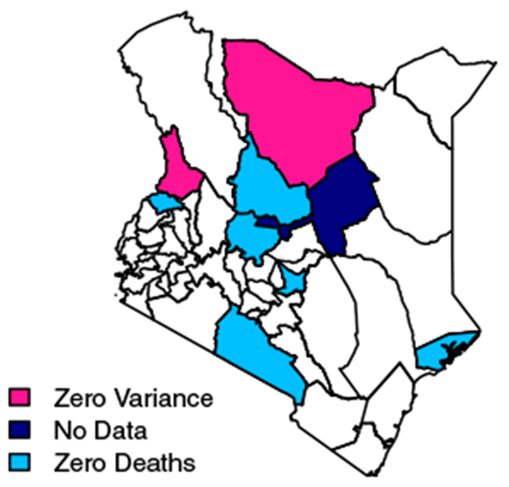
A map showing the areas whose estimates need adjusting from the KDHS 2003 for the period 1980 to 1984

FIGURE A2.

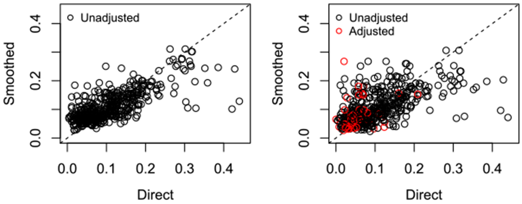
Comparison of direct and smooth estimates when we throw out observed zeroes (Left) or adjust them (Right)

APPENDIX B. HIV BIASES BY SURVEY AND REGION

This section shows figures of HIV adjustments⁵⁰ used for each Admin-1 area and each region in Kenya. While we make estimates of child mortality on the Admin-2 level, we must make the same HIV adjustments for all Admin-2 areas within an Admin-1 area, as that is the finest level for which Spectrum⁵⁷ makes estimates of the necessary inputs. For Malawi, we only have national HIV adjustments. The estimate reported in these plots is (1% children dead born to mothers missing) due to HIV/AIDS plotted against years before the survey. For FBH estimates in 5-year periods the point estimate plotted represents the adjustment for the 5-year period before the survey starting with that year, that is, the point at 20 years before a survey is the adjustment to be used for estimates made for 20 to 24 years before a survey. For SBH estimates, we use adjustments for single years before the survey. We use these adjustments to inflate the point estimates prior to smoothing,

FIGURE B1.

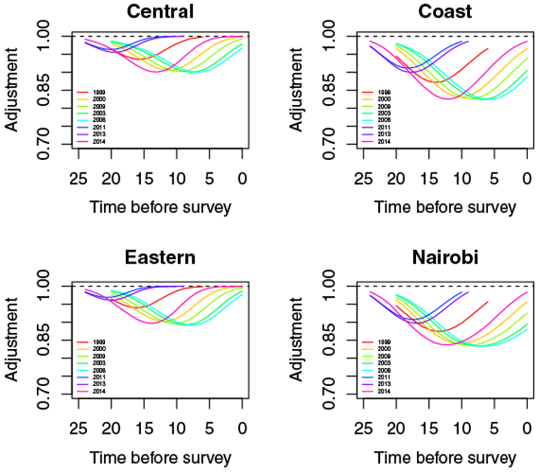
HIV adjustments for Central, Coast, Eastern regions and Nairobi

FIGURE B2.

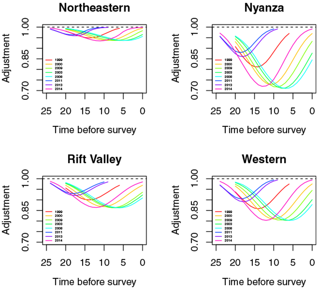
HIV adjustments for Northeastern, Nyanza, Rift Valley, and Western regions

FIGURE B3.

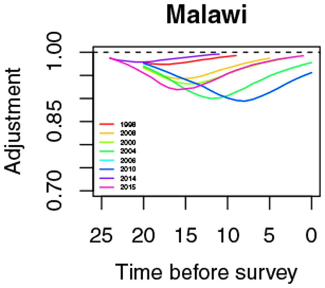
HIV adjustments for Malawi

$${}_{60}{\widehat{q}}_{0\mathrm{HIV}}^{its}=\frac{{}_{60}{\widehat{q}}_0^{its}}{1\%\mathrm{mothers\; missing}}.$$ (B1)

The delta method is used to adjust the variance estimate. One can see that the severity of the epidemic varies widely by Admin-2 area.

APPENDIX C. BIAS IN TIME

FIGURE C1.

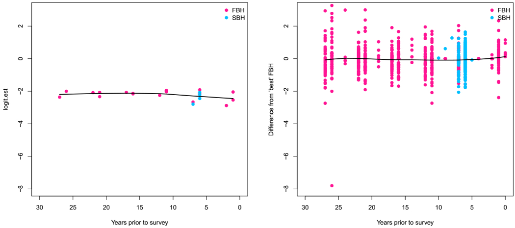
Bias on the logit scale for Kenya for each estimate plotted against the years prior to data collection for which the estimate applies. Left: national estimates. Right: Admin-2 level estimates. Black line is a loess smooth applied to the biases in either panel

APPENDIX D. HYPERPARAMETERS AND MODEL PARAMETERS

TABLE D1.

Proportion of variation as determined by marginal median variances for different random components.

Parameter	Median	Proportion
Kenya	ICAR	0.124	32.57
	IID Area	0.005	1.23
	RW2	0.093	24.38
	IID Time	0.002	0.44
	Interaction	0.158	41.38
Malawi	ICAR	0.017	6.92
	IID Area	0.000	0.20
	RW2	0.212	85.84
	IID Time	0.003	1.03
	Interaction	0.015	6.02

FIGURE D1.

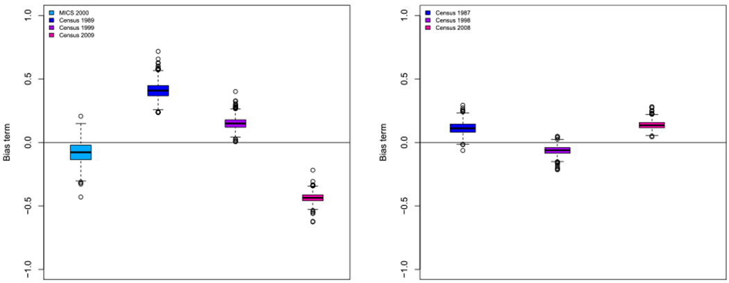
Marginal posterior distribution of the bias term (β_s) for each summary birth history data source in Kenya (Left) and Malawi (Right)

APPENDIX E. PERCENT REDUCTION

Prior to the SDGs, the United Nations’ Millennium Development Goals (MDGs) also called for progress in child mortality. In particular, MDG 4 set a goal of a two-thirds reduction in child mortality between 1990 and 2015. Nationally, we find a median proportion reduction of 62%, with 25th and 75th percentiles of 57% and 65%, respectively. In Figures E1 and E2 we see the subnational distribution of achievement of the MDG 4 goals. We present a conservative (25th percentile), a median, and an optimistic (75th percentile) estimate of the percent reduction by county. Admin-2 areas in white and blue have achieved the MDG by the respective measure in the plot. We find a median of 14 out of 47 counties in Kenya have achieved the MDG; the 25th and 75th percentiles are 7 and 24 counties, respectively. This contradicts strongly the findings of Macharia et al,⁵⁸ who find that no county in Kenya achieved the MDG by 2015. This discrepancy is likely due to the fact that their method does not account for the HIV epidemic in Kenya, and, thus, underestimates mortality going back in time. This leads to a smaller estimated reduction. In Malawi, we find that a median of 21 out of 28 districts have achieved the MDG by 2015. The conservative 25th percentile estimate shows 21 districts achieving the reduction goal, and an optimistic 75th percentile estimate has 22 districts reaching the MDG goal.

FIGURE E1.

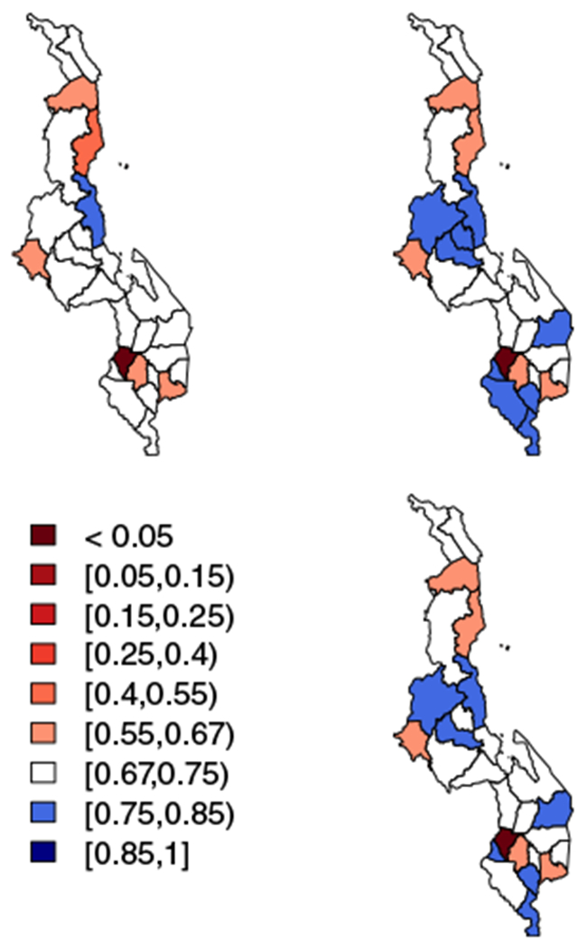
Top left: 25th percentiles of the distribution of reduction in under-five mortality rate from 1990 to 2015 in each district in Malawi. Top right: 75th percentiles of the distribution of reduction in each district. Bottom right: median percentiles of the distribution of reduction in each district. Areas in red have not achieved the Millennium Development Goal by 2015, with the color darkening as the percent reduction gets smaller. All other areas have achieved the goal, with white areas having an estimated percent reduction of 67% to 75% and areas in shades of blue having increasingly higher percent reduction as the blue shade darkens

FIGURE E2.

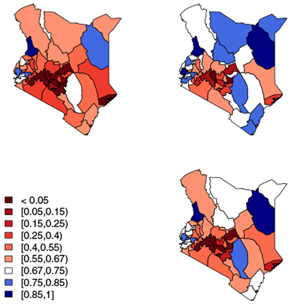
Top left: 25th percentiles of the distribution of reduction in under-five mortality rate from 1990 to 2015 in each county in Kenya. Top right: 75th percentiles of the distribution of reduction in each county. Bottom right: median percentiles of the distribution of reduction in each county. Areas in red have not achieved the Millennium Development Goal by 2015, with the color darkening as the percent reduction gets smaller. All other areas have achieved the goal, with white areas having an estimated percent reduction of 67% to 75% and areas in shades of blue having increasingly higher percent reduction as the blue shade darkens

APPENDIX F. NATIONAL RESULTS

Results of temporal smoothing model below for national direct and Brass estimates. Note: the Kenya MICS 2011 and 2013 provide estimates for only a small number of Admin-2 areas and, thus, are not included in the national analysis for Kenya. Figures F1 and F2 show period and yearly results with corresponding 95% intervals. In grey solid lines and dashed lines, respectively, are UN and IHME estimates for comparison. The national model below does not have any spatial components, but is otherwise analogous to the spatiotemporal model.

$$\begin{gathered} \mathrm{logit}({}_{60}{\widehat{q}}_0^{it})|{\eta }_{ts}\sim N({\eta }_{ts},{\kappa }_s^{-1}\times {\widehat{V}}^{ts}), \\ {\eta }_{ts}=\mu +\sum _s{\beta }_s\mathbf{1}(s\text{is SBH})+{\alpha }_t+{\gamma }_t. \end{gathered}$$ (F1)

FIGURE F1.

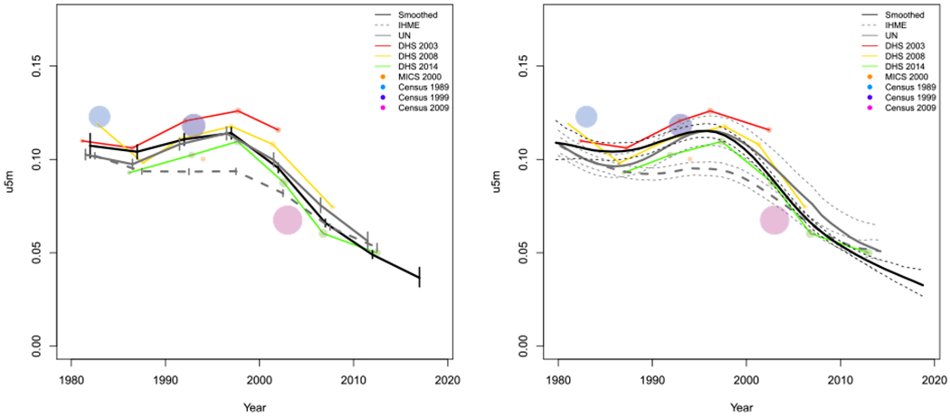
National results for Kenya. Left: Five-year period smoothed results in black with larger data points for estimates with larger precision in color. Right: Yearly smoothed results in black

FIGURE F2.

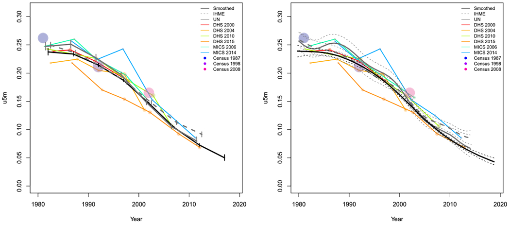
National results for Malawi.Left: Five-year period smoothed results in black with larger data points for estimates with larger precision in color. Right: Yearly smoothed results in black

APPENDIX G.

FIGURE G1.

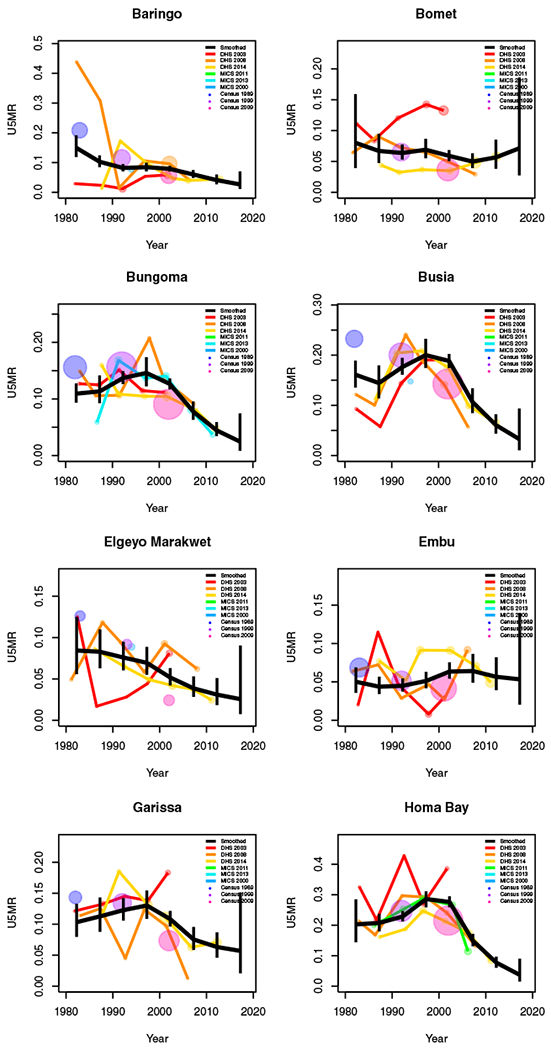
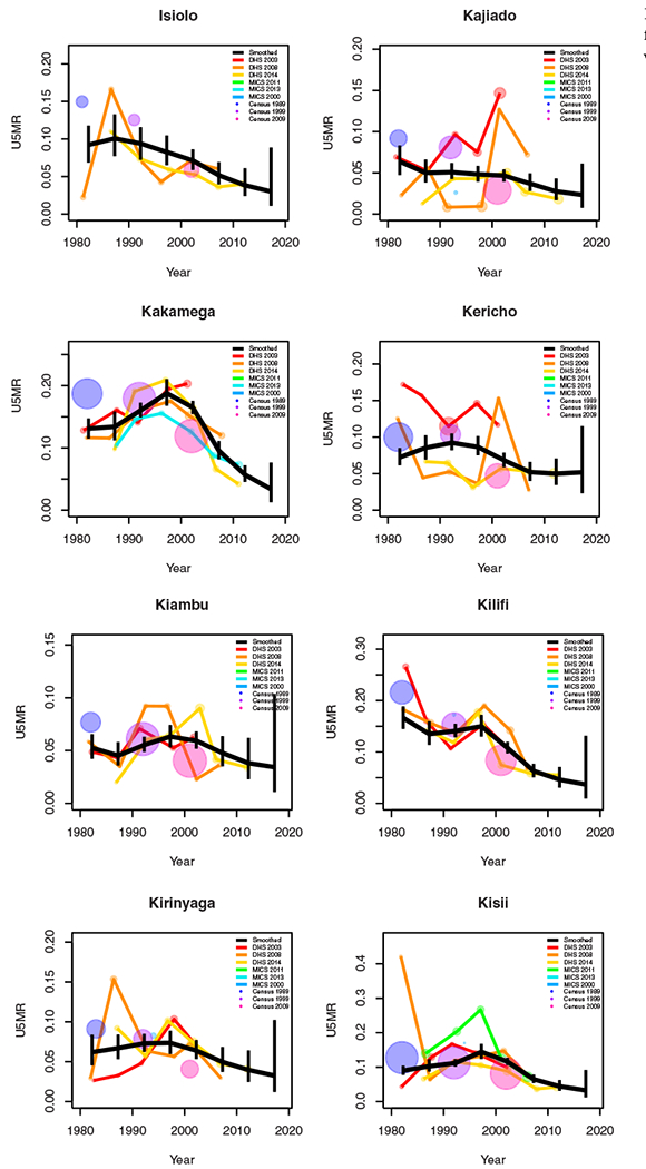
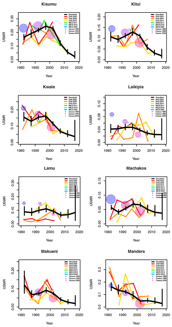
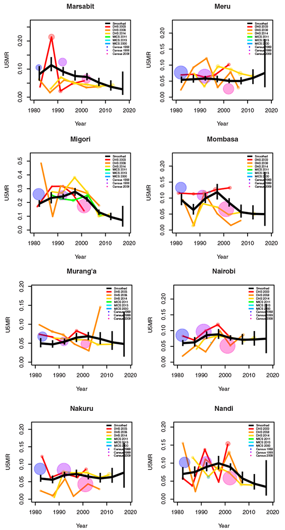
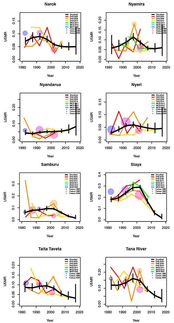
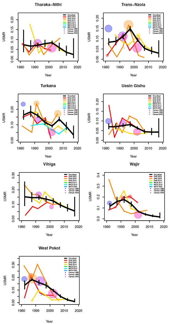
Period results by area: Kenya

APPENDIX H.

FIGURE H1.

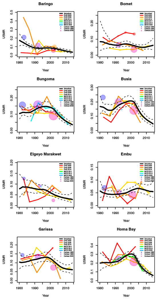
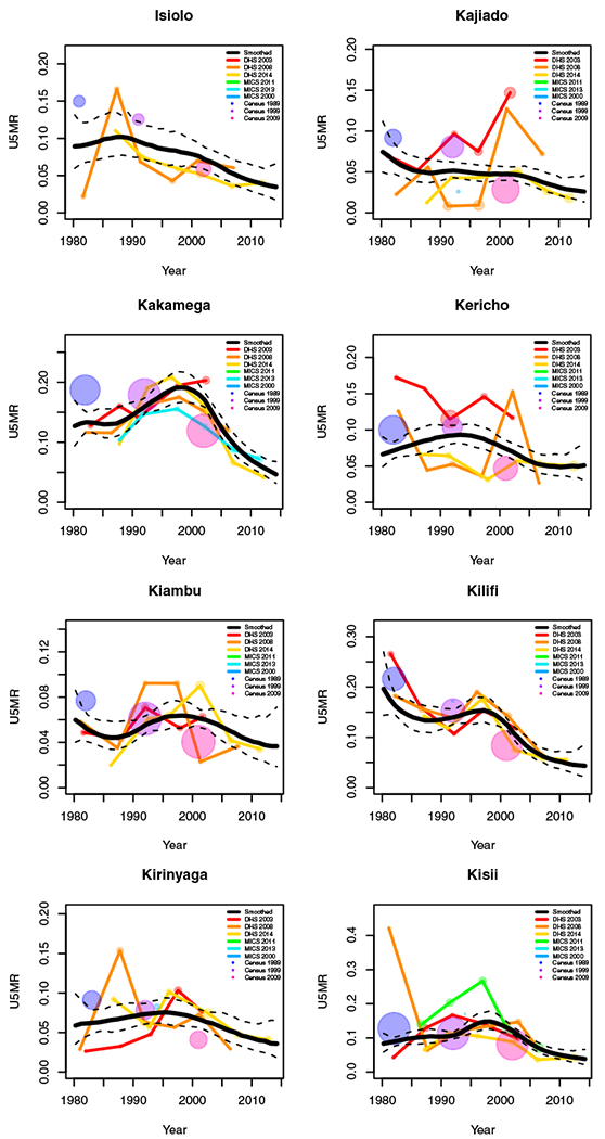
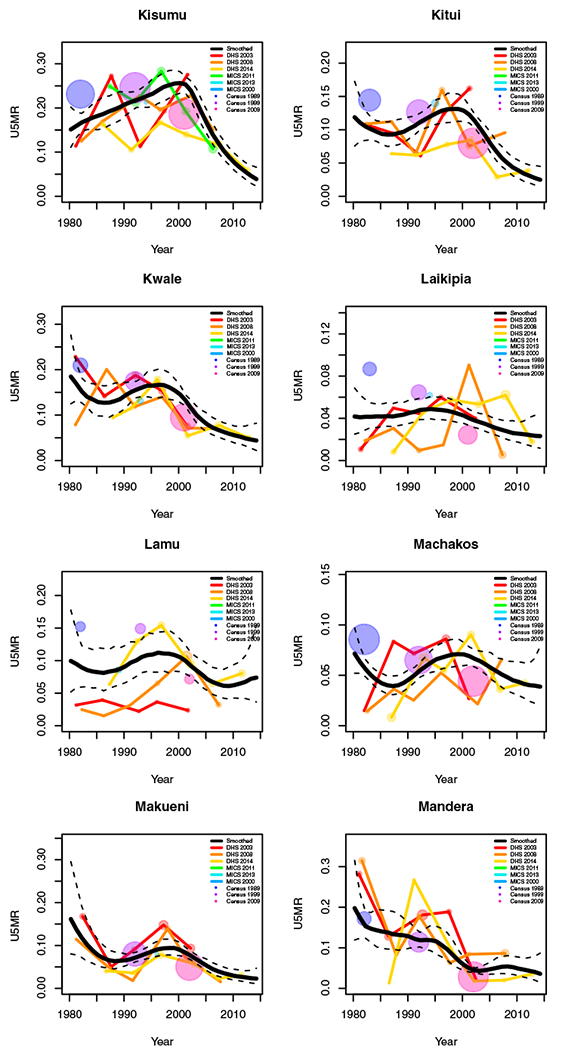
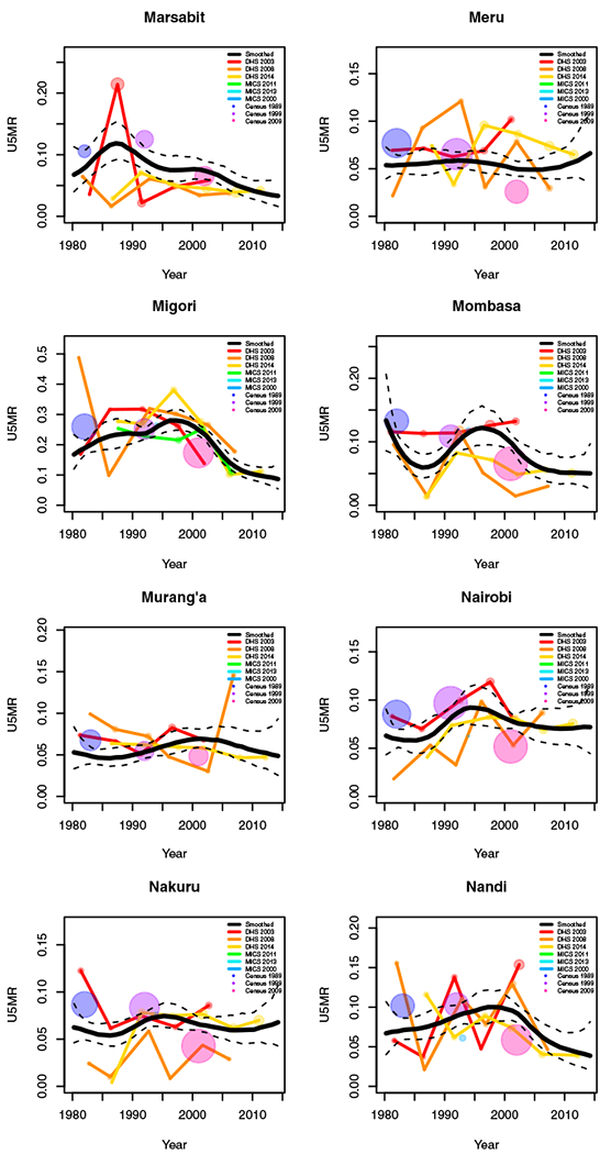
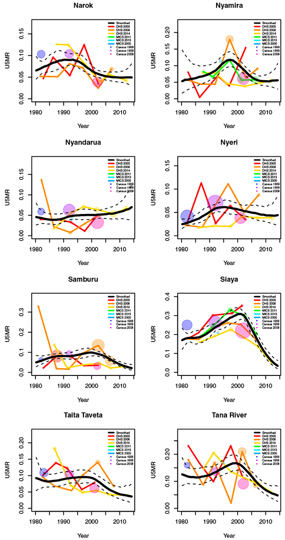
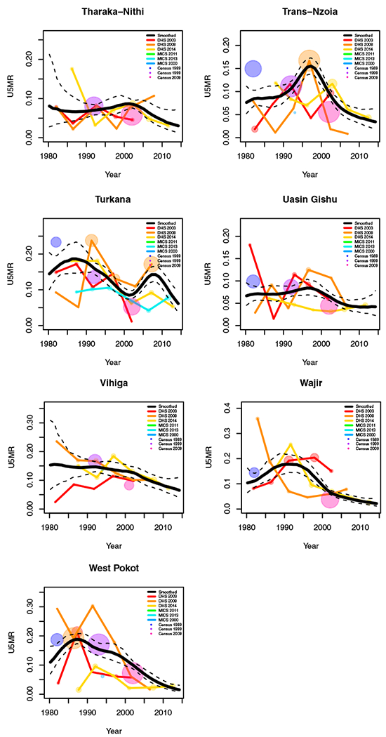
Yearly results by area: Kenya

APPENDIX I.

FIGURE I1.

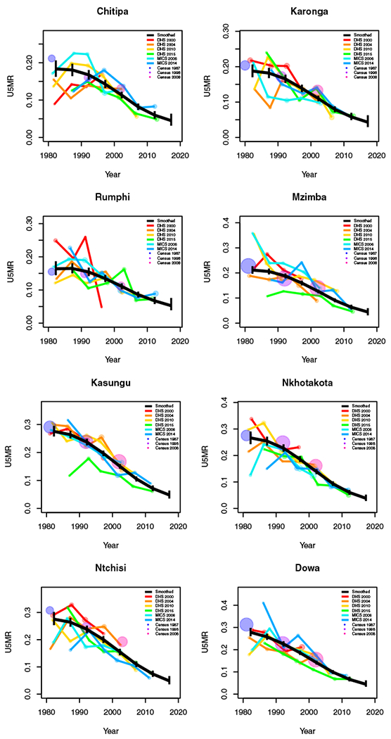
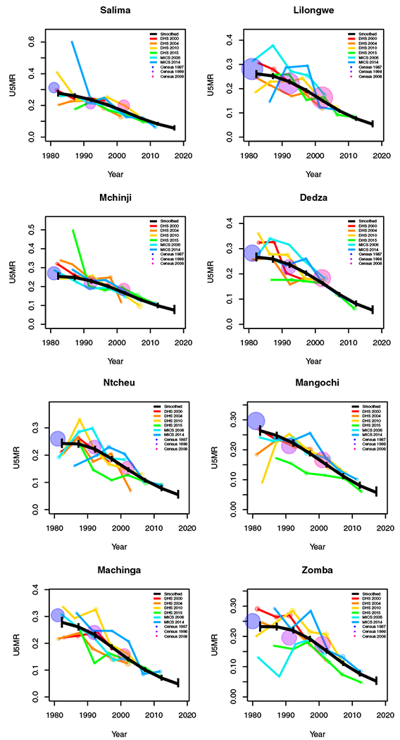
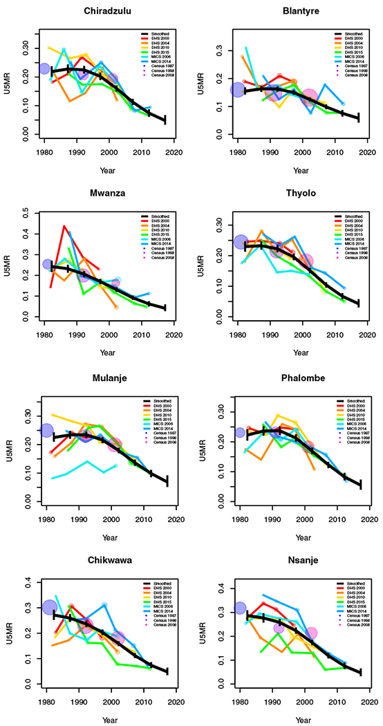
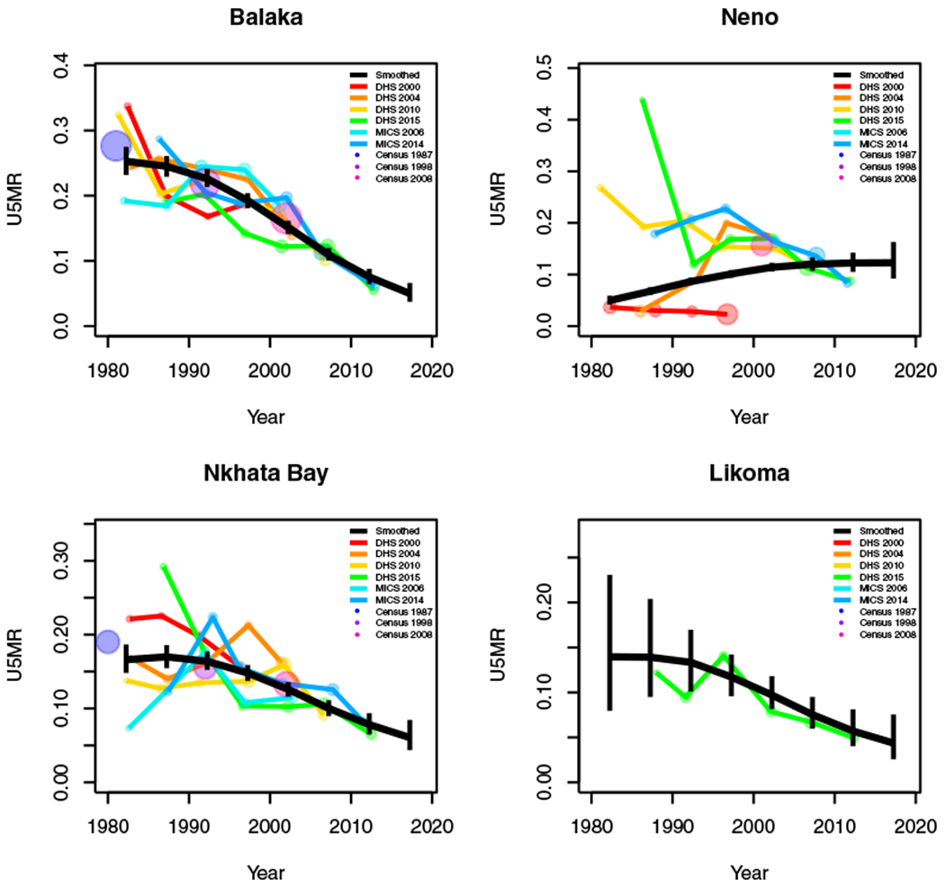
Period results by area: Malawi

APPENDIX J.

FIGURE J1.

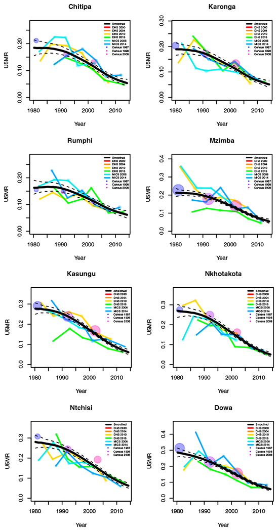
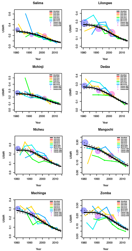
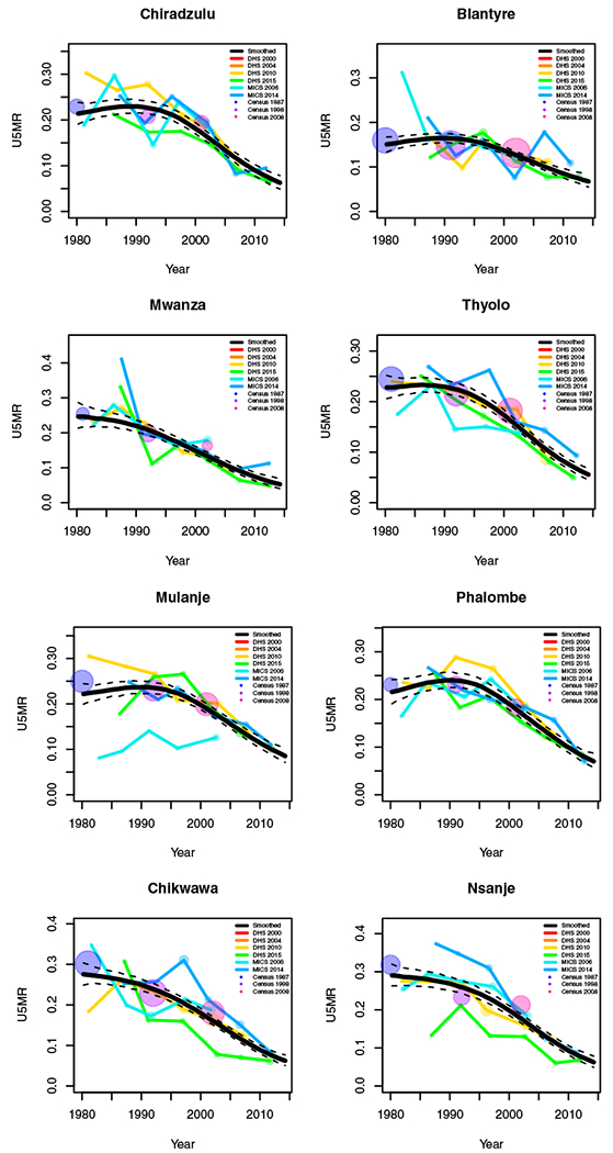
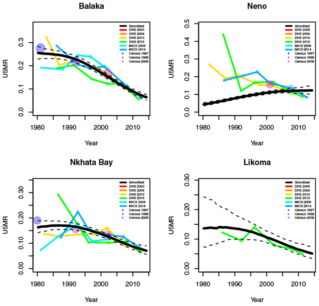
Yearly results by area: Malawi

REFERENCES

- 1.UN General Assembly. report of the open working group of the general assembly on sustainable development goals. General Assembly Document A/69/970, New York, NY; 2014:12. [Google Scholar]
- 2.ICF International. Demographic and health surveys (various) [Datasets]. funded by USAID 2004-2017. [Google Scholar]
- 3.UNICEF - Statistics and monitoring. Multiple indicator cluster surveys (MICS) [Datasets]. https://mics.unicef.org/surveys. [Google Scholar]
- 4.Alkema L, New J. Global estimation of child mortality using a Bayesian B-spline bias-reduction model. Ann Appl Stat. 2014;386:2122–2149. [Google Scholar]
- 5.Mercer L, Wakefield J, Pantazis A, Lutambi A, Masanja H, Clark S. Space–time smoothing of complex survey data: small area estimation for child mortality. Ann Appl Stat. 2015;9:1889–1905. [DOI] [PMC free article] [PubMed] [Google Scholar]
- 6.Li Z, Hsiao Y, Godwin J, Martin B, Wakefield J, Clark S. Changes in the spatial distribution of the under-five mortality rate: small-area analysis of 122 DHS surveys in 262 subregions of 35 countries in Africa. PLoS One. 2019;14:e0210645. [DOI] [PMC free article] [PubMed] [Google Scholar]
- 7.Kenya National Bureau of Statistics and Ministry of Health and National AIDS Control Council and Kenya Medical Research Institute and National Council for Population and Development. Kenya Demographic and Health Survey 2014; 2015.
- 8.Kenya National Bureau of Statistics and National AIDS Control Council and National AIDS/STD Control Programme and Ministry of Public Health and Sanitation, and Kenya Medical Research Institute. Kenya Demographic and Health Survey 2008-2009; 2010.
- 9.Central Bureau of Statistics and Ministry of Health and ORC Macro. Kenya Demographic and Health Survey 2003; 2004.
- 10.National Statistics Office and ICF. Malawi Demographic and Health Survey 2015-2016; 2017.
- 11.National Statistics Office and ICF Macro. Malawi Demographic and Health Survey 2010; 2011.
- 12.National Statistics Office and ORC Macro. Malawi Demographic and Health Survey 2004; 2005.
- 13.National Statistics Office and ORC Macro. Malawi Demographic and Health Survey 2000; 2001.
- 14.Minnesota Population Center. Integrated Public Use Microdata Series, International: Version 7.2 [Datasets]; 2019. 10.18128/D020.V7.2. [DOI] [Google Scholar]
- 15.Fay RE, Herriot RA. Estimates of income for small places: an application of James-Stein procedures to census data. J Am Stat Assoc. 1979;74:269–277. [Google Scholar]
- 16.Battese GE, Harter RM, Fuller WA. An error-components model for prediction of county crop areas using survey and satellite data. J Am Stat Assoc. 1988;83:28–36. [Google Scholar]
- 17.Wakefield J, Fuglstad GA, Riebler A, Godwin J, Wilson K, Clark SJ. Estimating under-five mortality in space and time in a developing world context. Stat Methods Med Res. 2019;28:2614–2634. [DOI] [PMC free article] [PubMed] [Google Scholar]
- 18.Brass W Uses of census or survey data for the estimation of vital rates. United Nations 1964. Paper prepared for the African Seminar on Vital Statistics; December 14-19, 1964. Addis Ababa. [Google Scholar]
- 19.UNICEF Levels and Trends in Child Mortality, Report 2019. Technical Report United Nations Children’s Fund; New York, NY; 2019. [Google Scholar]
- 20.Pedersen J, Liu J. Child mortality estimation: appropriate time periods for child mortality estimates from full birth histories. PLoS Med. 2012;9:e1001289. [DOI] [PMC free article] [PubMed] [Google Scholar]
- 21.Croft TN, Marshall AM, Allen CK. Guide to DHS Statistics: DHS-7. Rockville, Maryland: ICF; 2018. [Google Scholar]
- 22.Burstein R, Henry NJ, Collison ML, et al. Mapping 123 million neonatal, infant and child deaths between 2000 and 2017. Nature. 2019;574:353–358. [DOI] [PMC free article] [PubMed] [Google Scholar]
- 23.Elkasabi M Calculating fertility and childhood mortality rates from survey data using the DHS rates R package. PLoS One. 2019;14:1–22. [DOI] [PMC free article] [PubMed] [Google Scholar]
- 24.Allison P Event History and Survival Analysis. Vol 46. 2nd ed. Beverly Hills, CA: SAGE Publications; 2014. https://books.google.com/books?hl=en&lr=&id=XkACeUEiEsUC&oi=fnd&pg=PA5&dq=allison+event+history+analysis&ots=K5n1exDLIq&sig=AFd-G5R_qg60wN7Btua-yts_UH0#v=onepage&q=allison%20event%20history%20analysis&f=false. [Google Scholar]
- 25.Binder D On the variances of asymptotically normal estimators from complex surveys. Int Stat Rev. 1983;51:279–292. [Google Scholar]
- 26.Lumley T Analysis of complex survey samples. J Stat Softw. 2004;9:1–19. [Google Scholar]
- 27.Rue H, Held L. Gaussian Markov Random Fields: Theory and Applications. Boca Raton, FL: CRC Press; 2005. [Google Scholar]
- 28.Besag J, York J, Mollie A. Bayesian image restoration with two applications in spatial statistics (with discussion). Ann Inst Stat Math. 1991;43:1–59. [Google Scholar]
- 29.Knorr-Held L Bayesian modelling of inseparable space-time variation in disease risk. Stat Med. 2000;19:2555–2567. [DOI] [PubMed] [Google Scholar]
- 30.Simpson D, Rue H, Riebler A, Martins T, Sørbye S. others. Penalising model component complexity: a principled, practical approach to constructing priors. Stat Sci. 2017;32:1–28. [Google Scholar]
- 31.Riebler A, Sørbye SH, Simpson D, Rue H. An intuitive Bayesian spatial model for disease mapping that accounts for scaling. Stat Methods Med Res. 2016;25:1145–1165. [DOI] [PubMed] [Google Scholar]
- 32.Rue H, Martino S, Chopin N. Approximate Bayesian inference for latent Gaussian models by using integrated nested Laplace approximations. J R Stat Soc Ser B. 2009;71:319–392. [Google Scholar]
- 33.Martins T, Simpson D, Lindgren F, Rue H. Bayesian computing with INLA: new features. Comput Stat Data Anal. 2013; 67:68–83. [Google Scholar]
- 34.Rajaratnam JK, Tran LN, Lopez AD, Murray CJ. Measuring under-five mortality: validation of new low-cost methods. PLoS Med. 2010;7:e1000253. [DOI] [PMC free article] [PubMed] [Google Scholar]
- 35.Hill K, Brady E, Zimmerman L, Montana L, Silva R, Amouzou A. Monitoring change in child mortality through household surveys. PLoS One. 2015;10:e0137713. [DOI] [PMC free article] [PubMed] [Google Scholar]
- 36.Brady E, Hill K. Testing survey-based methods for rapid monitoring of child mortality, with implications for summary birth history data. PLoS One. 2017;12:e0176366. [DOI] [PMC free article] [PubMed] [Google Scholar]
- 37.Burstein R, Wang H, Reiner RC Jr, Hay SI. Development and validation of a new method for indirect estimation of neonatal, infant, and child mortality trends using summary birth histories. PLoS Med. 2018;15:e1002687. [DOI] [PMC free article] [PubMed] [Google Scholar]
- 38.Wilson K, Wakefield J. Child mortality estimation incorporating summary birth history data. Biometrics. 2020:1–11. https://onlinelibrary.wiley.com/action/showCitFormats?doi=10.1111%2Fbiom.13383. [DOI] [PubMed] [Google Scholar]
- 39.Hill K, Zlotnik H, Trussell J. Demographic estimation: a manual on indirect techniques. Manual X; 1983. [Google Scholar]
- 40.Preston SH, Heuveline P, Guillot M. Demography: Measuring and Modeling Population Processes. Blackwell Malden, MA: 2000. [Google Scholar]
- 41.Li Z, Martin B, Dong T, et al. Space-time smoothing of demographic and health indicators using the R package SUMMER; 2020. https://arxiv.org/abs/2007.05117. [Google Scholar]
- 42.Hill K, Trussell J. Further developments in indirect mortality estimation. Popul Stud. 1977;31:313–334. [DOI] [PubMed] [Google Scholar]
- 43.Coale A, Trussell J, Annex I. estimating the time to which Brass estimates apply. Popul Bull UN. 1977;10:87–89. [PubMed] [Google Scholar]
- 44.Trussell TJ. A re-estimation of the multiplying factors for the Brass technique for determining childhood survivorship rates. Popul Stud. 1975;29:97–107. [DOI] [PubMed] [Google Scholar]
- 45.Coale A, Demeny P. Regional Model Life Tables and Stable Populations. Princeton, NJ: Princeton University Press; 1966. [Google Scholar]
- 46.Hill K, You D, Inoue M, Oestergaard MZ. Child mortality estimation: accelerated progress in reducing global child mortality, 1990–2010. PLoS Med. 2012;9:1–11. [DOI] [PMC free article] [PubMed] [Google Scholar]
- 47.Ha NS, Lahiri P, Parsons V. Methods and results for small area estimation using smoking data from the 2008 national health interview survey. Stat Med. 2014;33:3932–3945. [DOI] [PubMed] [Google Scholar]
- 48.Sugasawa S, Kubokawa T, Rao J. Small area estimation via unmatched sampling and linking models. Test. 2018;27:407–427. [Google Scholar]
- 49.Wolter K Introduction to Variance Estimation. 2nd ed. Berlin, Germany: Springer Science & Business Media; 2007. [Google Scholar]
- 50.Walker N, Hill K, Zhao F. Child mortality estimation: methods used to adjust for bias due to AIDS in estimating trends in under-five mortality. PLoS Med. 2012;9:1–7. [DOI] [PMC free article] [PubMed] [Google Scholar]
- 51.Stover J, Brown T, Marston M. Updates to the Spectrum/Estimation and Projection Package (EPP) model to estimate HIV trends for adults and children. Sex Transm Infect. 2012;88:1–6. [DOI] [PMC free article] [PubMed] [Google Scholar]
- 52.Pezzulo C, Bird T, Utazi E, et al. Geospatial modeling of child mortality across 27 countries in Sub-Saharan Africa DHS Spatial Analysis Reports No. 13; 2016.
- 53.Golding N, Burstein R, Longbottom J, et al. Mapping under-5 and neonatal mortality in Africa, 2000–15: a baseline analysis for the Sustainable Development Goals. Lancet. 2017;390:2171–2182. [DOI] [PMC free article] [PubMed] [Google Scholar]
- 54.Lindgren F, Rue H, Lindström J. An explicit link between Gaussian fields and Gaussian Markov random fields: the stochastic differential equation approach (with discussion). J Royal Stat Soc Ser B. 2011;73:423–498. [Google Scholar]
- 55.Wilson K, Wakefield J. Pointless spatial modeling. Biostatistics. 2018;21:e17–e22. [DOI] [PMC free article] [PubMed] [Google Scholar]
- 56.Wakefield J, Okonek T, Pedersen J. Small area estimation for disease prevalence mapping. Int Stat Rev. 2020;88(2):398–418. [DOI] [PMC free article] [PubMed] [Google Scholar]
- 57.UNAIDS Quick Start Guide for Spectrum (Downloaded December 2015). UNAIDS; 2014. [Google Scholar]
- 58.Macharia PM, Giorgi E, Thuranira PN, et al. Subnational variation and inequalities in under-five mortality in Kenya since 1965. BMC Publ Health. 2019;19:146. [DOI] [PMC free article] [PubMed] [Google Scholar]