Linking excess mortality to mobility data during the first wave of COVID-19 in England and Wales

Abstract

Non-pharmaceutical interventions have been implemented worldwide to curb the spread of COVID-19. However, the effectiveness of such governmental measures in reducing the mortality burden remains a key question of scientific interest and public debate. In this study, we leverage digital mobility data to assess the effects of reduced human mobility on excess mortality, focusing on regional data in England and Wales between February and August 2020. We estimate a robust association between mobility reductions and lower excess mortality, after adjusting for time trends and regional differences in a mixed-effects regression framework and considering a five-week lag between the two measures. We predict that, in the absence of mobility reductions, the number of excess deaths could have more than doubled in England and Wales during this period, especially in the London area. The study is one of the first attempts to quantify the effects of mobility reductions on excess mortality during the COVID-19 pandemic.

Highlights

• •We link digital trace data to excess mortality during the first wave of COVID-19.
• •A relationship between reduced mobility and lower mortality emerges after five weeks.
• •Governmental measures may have prevented almost 95,000 deaths in England and Wales.

1. Introduction

After the first cases of COVID-19 were identified in Wuhan City, China, in December 2019, the outbreak rapidly spread globally reaching pandemic proportions. As of January 31, 2021, over 100 million cases of infections and 2.2 million deaths have been reported worldwide (World Health Organization, 2021), although these values are likely underestimated due to cross-country differences in disease monitoring and reporting, asymptomatic cases, medically unattended cases, and deaths indirectly related to COVID-19 (Havers et al., 2020; Pullano et al., 2021).

Local and national governments across the globe implemented various non-pharmaceutical interventions (NPIs) aimed at reducing human mobility and close contacts in the population and, consequently, the probability of transmission of the SARS-CoV-2 virus. These measures include travel bans, cancellations of public gatherings, social distancing, school closures, recommendations to work from home and stay at home, and nationwide lockdowns (Brauner et al., 2020; Hale et al., 2020). In Europe, such interventions were introduced in the first half of 2020, with considerable cross-country differences in terms of strictness, timing and duration. Most of these measures were then lifted during the summer as the number of new infections and deaths declined, but also to alleviate their long-term socioeconomic costs on society and citizens. A second wave of infections and deaths prompted the re-introduction of NPIs after the summer, again with different strategies across Europe (Kupferschmidt, 2020).

A growing body of literature has documented the link between the introduction of NPIs and the reduction of the SARS-CoV-2 virus’ transmission (Brauner et al., 2020; Davies et al., 2020; Dehning et al., 2020; Flaxman et al., 2020; Hsiang et al., 2020) and the human cost - in terms of infections and deaths - of letting the virus spread unchecked (Buss et al., 2021). However, it still remains unclear how to measure the effectiveness of such interventions in alleviating the mortality burden of COVID-19. Estimating the impact of NPIs on mortality reductions is critical for policy makers to make informed decisions, in the context of both current and future pandemics.

In this article, we study the relationship between human mobility and excess mortality at the sub-national level in England and Wales during the first wave of the COVID-19 pandemic, specifically from February 15 to August 14, 2020. Note that at the time of writing (February 2021), the second wave of infections and deaths is still unfolding in the UK and the inclusion of these data could lead to misleading findings. Approximately 51,500 COVID-19 deaths were registered during this period of time (Office for National Statistics, 2020b), which includes almost one month before any NPIs were put in place. The British government applied various mobility restrictions strategies between March 12 and 24, 2020, including encouragement of social distancing, closure of schools, ban of public events, and total lockdown (Cameron-Blake et al., 2020; Flaxman et al., 2020). The goal of this paper is to estimate the impact of these governmental decisions, and consequent reduction in human movements, on excess all-cause mortality.

Human mobility plays a key role in the spread of infectious diseases (Riley, 2007; Tatem et al., 2006; Wilson, 1995). In our contemporary societies, where millions of people travel and commute every day within and across cities and regions, infectious diseases have the opportunity to spread more rapidly, and on a larger scale, than ever before. Population movement can in fact increase the disease prevalence by introducing new pathogens into susceptible populations, or by increasing social contacts between susceptible and infected individuals (Wesolowski et al., 2016). Timely, accurate, and comparative data on human mobility are therefore critical for informing public health interventions, but generally not available or easily accessible, and the ongoing COVID-19 pandemic has once again amplified this long-standing issue. Recent work has highlighted the potential benefits of harnessing geo-located smartphone data to inform policy makers (Oliver et al., 2020) and to assess the impact of mobility restrictions on social distancing in near real-time (Badr et al., 2020; Davies et al., 2020; Pepe et al., 2020; Schlosser et al., 2020).

In this study, we exploit a publicly available human mobility dataset, the Google COVID-19 Mobility Reports (GCMR) (Google LLC, 2021). The GCMR reports changes in mobility of Google Maps users across different categories (e.g. supermarkets and pharmacies, workplaces, residential areas) with respect to the start of 2020. This dataset has been leveraged to monitor national mobility in the United Kingdom following the implementation of NPIs (Drake et al., 2020), and it has been employed (alongside social contacts data) to estimate the effect of tiered restrictions in England and the lockdown in Wales implemented in October 2020 (Davies et al., 2020).

We model the association between the reduction in human mobility and the excess all-cause mortality during the first wave of the COVID-19 pandemic. Given the high uncertainty surrounding the number of infections and deaths, we choose to estimate excess mortality, which indicates the number of deaths above what would be expected in a non-crisis period. This measure overcomes potential issues of incorrect death classification and registration, and is largely considered the best indicator of the pandemic's impact on mortality (Kontis et al., 2020; National Academies of Sciences, Engineering, and Medicine, 2020). Given that changes in mobility are not immediately reflected in changes in mortality, we analyse different time lags between the two measures to calibrate the length of the expected delay in the effect of mobility restrictions on mortality. We expect reduction in mobility to first decrease the number of close social contacts in the population, leading to fewer new infections and, eventually, fewer deaths.

2. Material and methods

2.1. Data

We employ two data sources in our study: the UK Office for National Statistics (ONS) for mortality and population data, and the Google COVID-19 Community Mobility Reports (GCMR) for mobility data.

The ONS reports the weekly number of deaths registered in England and Wales, broken down by age group, sex and region of usual residence (Office for National Statistics, 2021). In the ONS classification, weekly data do not refer to calendar weeks, but to rolling 7-day periods, from Saturday to Friday, and we keep this notation throughout the article. For our purposes, we retrieve the weekly number of deaths by region for the years 2015–2020. We consider a total of ten regions based on the NUTS-1 (Nomenclature of Territorial Units for Statistics) subdivision, namely Wales plus nine regions in England (North East, North West, Yorkshire and The Humber, East Midlands, West Midlands, East, London, South East and South West). We focus our analysis on the first wave of the COVID-19 pandemic, hence we use data until week 2020–33 (i.e. until August 14, 2020). We obtain data on total population in each region for the years 2015–2019 from the ONS (Office for National Statistics, 2020a).

The GCMR reports daily mobility data in six categories of location: residential, workplaces, supermarket and pharmacy (grocery), transit, retail, and parks (Google LLC, 2021). Data are provided as percentage variations in number of visits or time spent in each category, relative to a pre-COVID-19 baseline period, defined from January 3 to February 6, 2020. The baseline period is defined by Google and cannot be modified. The data account for weekly seasonality of movement by estimating a set of seven baseline weekdays using the median value for each particular weekday during the 5-week baseline period. Daily relative change is estimated as the percentage change with respect to the corresponding baseline weekday for any given report date. To protect users’ privacy, absolute mobility values are not available.

We obtain mobility data for each category of the GCMR for 108 sub-national regions (the GCMR's sub_region_1 variable), covering a geographic area inhabited by 99% of the population of England and Wales, from February 15 (the first available date in the dataset) to August 14, 2020. We aggregate the GCMR data by week (from Saturday to Friday, for consistency with mortality data) and region (taking the weighted average across all counties belonging to a given region, with weights equal to their population sizes) to make it comparable to the mortality data.

Relying on a fixed baseline period ignores yearly seasonality of movement, which may be affected by weather patterns, national holidays, vacation periods, etc. Important bank holidays, extreme weather events, or other major events during the 5-week long baseline period can affect the estimates of future relative changes in visits to grocery stores. We have no access to the raw mobility data used to produce the GCMR, but we find no evidence of any major events in England or Wales that could have systematically biased the Google mobility data during the baseline period. Furthermore, the baseline week is based on the median value, which would be largely unaffected by short-lived temporary fluctuations in absolute mobility values. Finally, the baseline period is not affected by restrictions on movement, which where first introduced on March 12, 2020.

2.2. Computing excess mortality

Weekly mortality data generally show strong seasonal behavior. As such, we opt for a modulation model that accounts for seasonal patterns using week-specific coefficients for the death counts.

For a given region, let $\mathit{D}=\left(d_{w,t}\right)$ denote a matrix containing the registered number of deaths in week $w=1,\dots ,53$ and year $t=2015,\dots ,2020$, i.e., weekly registered deaths from week 2015–01 to week 2020–33. In alternative to the conventional Poisson distribution, we assume that the $d_{w,t}$ are realisations of a random variable $D_{w,t}$ that follows a Negative Binomial distribution. We thus allow for the overdispersion typically displayed in mortality data, i.e., the variance associated with the process is expected to be larger than what would be implied by the expected value in a Poisson model. One of the main sources of overdispersion in the data is likely the unobserved heterogeneity stemming from the varying strength of the seasonal pattern, which is related to the yearly variation of influenza epidemics (Rau, 2007).

Let ${\mu }_{w,t}=\mathbb{E}\left(D_{w,t}\right)$ denote the expected value of the Negative Binomial process. We model the expected number of deaths using a Generalized Additive Model (GAM) with logarithmic link, exposures as offset, and time-specific covariates:

$$\text{ln}\left({\mu }_{w,t}\right)=\text{ln}\left(e_{w,t}\right)+f\left(x_{w,t}\right)+{\alpha }_0+{\alpha }_w,$$ (1)

where $e_{w,t}$ denotes the exposure to the risk of death, the function $f(\cdot )$ is a smooth function over the time-points $x_{w,t}=1,\dots ,m$, where m denotes the total number of observations, ${\alpha }_0$ is an intercept and ${\alpha }_w$ are week-specific coefficients. To ensure identifiability of the ${\alpha }_w$ coefficients, the first week is taken as the reference group (i.e. ${\alpha }_1=1$). Exposures over weeks and years are obtained by linear interpolation of mid-year populations in years $t=2015,\dots ,2019$. For the year 2020, the mid-year population is still not available at the time of writing, therefore we keep constant the 2019 mid-year population given the impact of the COVID-19 pandemic on fertility, mortality and migration.

Whereas the coefficients ${\alpha }_w$ capture the typical pattern of mortality in registered week w (including seasonal behavior of weekly mortality data, periodic bank holidays effects, etc.), the smooth time component aims to describe long-term mortality trends. Given that mortality data are recorded by registration rather than occurrence, such a specification provides a better description of the data than including trigonometric functions for the seasonal pattern of deaths. Estimation of the model described in Equation (1) is performed in R (R Development Core Team, 2020) using the mgcv package (Wood, 2019, pp. 8–31).

For each region independently, we model data for the pre-pandemic period (from week 2015–01 to week 2020–06, corresponding to a total of $m=267$ observations) and predict the expected number of deaths ${\hat{d}}_w$ for the COVID-19 period (from week 2020–07 to week 2020–33). We use week 2020–06 as last estimated week before prediction for consistency with the Google mobility data, for which the baseline period runs from week 2020–02 to week 2020–06. Consequently, the effect of the pandemic is not captured by the time trend of the model, and ${\hat{d}}_{w,2020}$ for the predicted weeks could be interpreted as the number of deaths that would have occurred in 2020 in the absence of the COVID-19 pandemic.

This approach allows us to readily evaluate the excess number of deaths ${\hat{\delta }}_w$ for the weeks 07–33 in 2020 as the difference between the observed and the expected ones, i.e. ${\hat{\delta }}_w=d_w-{\hat{d}}_w$. In order to account for regional differences in population, we then compute the excess mortality rate, or per capita excess mortality, $y_w={\hat{\delta }}_w/e_w$, dividing excess deaths by the (extrapolated) region-specific exposures in week w of 2020.

In addition to fitting the GAM, we perform a sensitivity analysis on the computation of the excess mortality rate. In particular, we derive another estimate of $y_w$ by computing, for each week, the expected number of deaths as the average of the observed deaths between 2015 and 2019 (see Appendix B).

2.3. Combining google categories into a single index

For each region analysed in the paper, we aim to extract the most relevant signals from the different categories of the GCMR by merging them into a combined “Google mobility index”. Ideally, all three dimensions of the GCMR (Google categories, regions and time) should be considered simultaneously. This rules out region-independent principal component analysis (PCA) of the mobility data over time. A solution is instead given by a multilinear principal component analysis (MPCA) (Lu et al., 2008). In both approaches, the goal is to retain as much as possible the variation present in the original data set. However, whereas standard PCA reduces the dimensionality of a two-dimensional data set, MPCA allows to extract features of a multidimensional object such as the GCMR.

To do so, we construct a tensor object (a multidimensional array) containing the three types of data, and we extract the first component of the MPCA for the dimensions time and region. We thus obtain the combined Google index for each region over time retaining most of the information regarding the mobility during the period analysed. In R, this can be achieved by using the rTensor package (Li et al., 2018).

2.4. Modelling the relationship between excess mortality and mobility

Given the estimated excess mortality rate for each week and region, we intend to assess whether an association with the change in mobility exists, and its magnitude. The spread of COVID-19 mainly occurs through contacts between infectious and susceptible individuals (Zhang et al., 2020). Hence, a reduction in mobility should lead to a reduction in social contacts, then in the infection spread and, ultimately, in the COVID-related mortality. However, this process requires time, as we would expect the reduction in physical mobility observed today to possibly have an impact on the infection spread and the related mortality in the coming weeks. This calls for the introduction of a time lag of x weeks in the mobility data, which corresponds to the amount of time necessary for the change in mobility to have an impact on mortality. In other words, we analyse the relationship between excess mortality and changes in human mobility that occurred x weeks before. We do not choose the value of x a priori, but rather we determine its most plausible value from the regression analysis of our data (see Section 3.2).

Moreover, we work with rates that vary over weeks and for different regions. While the mortality trend will be assumed to remain constant in space, we need to account for the regional heterogeneity in excess mortality and response to mobility changes, given that data within each region are likely correlated. This setting calls for a mixed-effects modelling approach, since we aim to know whether an association between excess mortality and human mobility over time still exists, after controlling for the variation across regions.

Let $y_{r,w}$ denote the excess mortality rate for a given region r in week w. We model $y_{r,w}$ as follows:

$$y_{r,w}={\beta }_0+u_r+\left({\gamma }_0+{\gamma }_r\right)g_{r,w-x}+\sum _{s=1}^n{\beta }_s{B}_s\left(w\right)+{\epsilon }_{r,w},$$ (2)

where ${\beta }_0$ is the common intercept and $u_r$ are the region-specific random intercepts, added to capture average regional differences; ${\gamma }_0$ is the common mobility coefficient, which can be interpreted as the average change in per capita excess mortality for a unit change in the mobility indicator (with respect to the baseline period), and ${\gamma }_r$ are the region-specific random slopes that modify the effect of mobility change for region r during the (lagged) week $w-x$, i.e., $g_{r,w-x}$. Random intercepts $u_r$ and random slopes ${\gamma }_r$ are normally distributed with mean zero and variance ${\sigma }_u^2$ and ${\sigma }_{\gamma }^2$, respectively, with their dependence captured by the covariance term ${\sigma }_{u,\gamma }$, which allows the computation of a model-based correlation coefficient. Evidence for ${\sigma }_u^2$ and ${\sigma }_{\gamma }^2$ being greater than zero implies the existence of regional differences in the baseline levels of mortality and heterogeneity in the responses to mobility changes, respectively. The baseline mortality time trend is modelled in a flexible way using a non-parametric approach based on B-spline bases $B_s$, with ${\beta }_s$ denoting the associated coefficients. Finally, ${\epsilon }_{r,w}$ is the vector of the residuals, distributed as ${\epsilon }_{r,w}~N\left(0,{\sigma }^2\right)$ and assumed to be independent of the random effects $u_r$ and ${\gamma }_r$.

To account for uncertainty in the estimates, related to both the computation of excess mortality and the mixed-effects regression in our estimates, we employ a bootstrap approach to derive 95% pointwise confidence intervals for the model results. Specifically, we generate 1000 simulated death counts from the deviance residuals of the GAM; for each simulation, we compute the regression in Equation (2) and derive fitted excess mortality rates. We fit the model in R using the lme4 package (Bates et al., 2015), and we compute B-spline bases using the splines package (R Development Core Team, 2020).

Finally, all data and source codes necessary for the reproducibility of our results are available at the following repository: https://osf.io/4pfb7/.

3. Results

3.1. Time series of google mobility and excess mortality rate

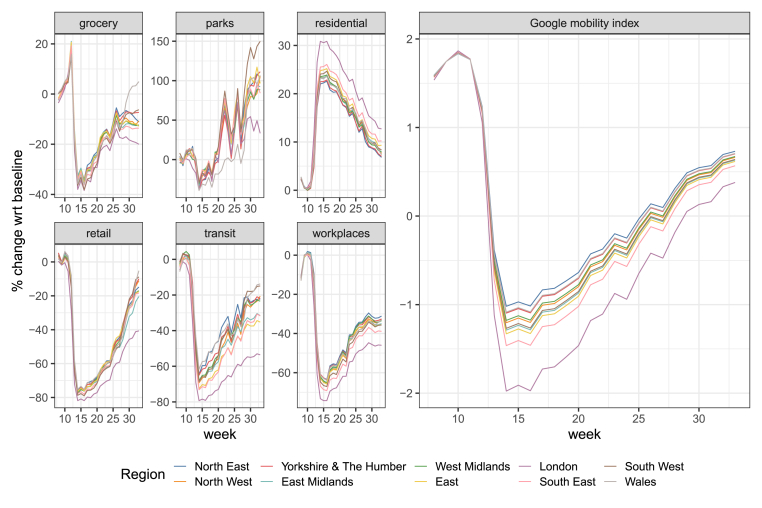
We start by computing the combined “Google mobility index” at the regional level in England and Wales during weeks 8–33 of 2020. Fig. 1 shows the six categories of the GCMR – supermarket and pharmacy (grocery), parks, residential, retail, transit, and workplaces – and the Google mobility index for each region. Strong mobility reductions from week 11 onwards – corresponding to the introduction of the NPIs – are clearly visible for the grocery, retail, transit and workplaces categories, as well as from the increase in time spent at residential locations.

Fig. 1.

Six categories of the GCMR and their combination into the Google mobility index in England and Wales by region during weeks 8–33 of 2020. Source: Authors' own elaboration based on data from Google LLC (2021).

In order to derive the combined indicator, we employ multilinear principal component analysis (MPCA) on five categories of the GCMR. We do not include the parks category in the MPCA for several reasons: (i) its pattern is different and more volatile than those of other categories, (ii) the category is subject to a higher proportion of missing data (see Fig. A.9 in Appendix A), and (iii) its inclusion decreases the amount of explained Frobenius norm (a measure comparable to the overall variance of the mobility data). The right panel of Fig. 1 shows that the Google index captures most of the peculiarities found in the GCMR. For example, mobility in the region of London decreased considerably more than in the other nine regions, and this is well captured by the Google index. The explained Frobenius norm of the MPCA amounts to 86.6%.

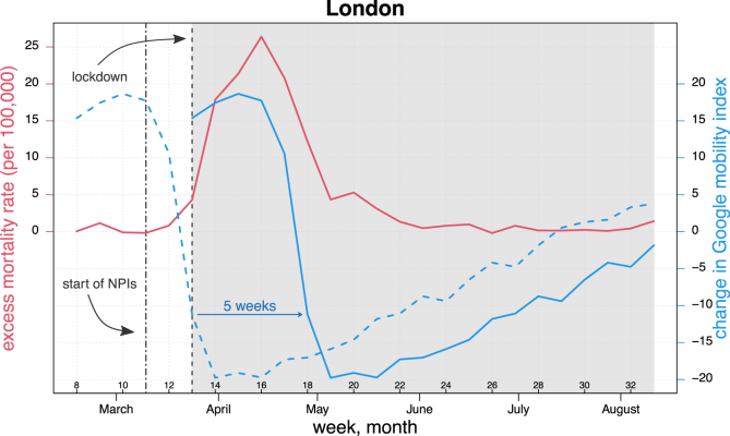
Next, we compute the excess mortality rate at the regional level during the same period of time. Fig. 2 shows the time series of the Google mobility index and the excess mortality rate in the region of London, plus: (i) a forward lag of five weeks for the mobility data, (ii) the time period that we will analyse in our regression framework (weeks 13–33, highlighted in the grey shaded area), and (iii) the start of NPIs on March 12 (week 11) and the enforcement of the lockdown on March 24 (week 13).

Fig. 2.

Time series of excess mortality rate per 100,000 individuals (red line) and change in Google mobility index at week t (dashed blue line) and with a five-week forward shift (solid blue line) in the region of London during weeks 8–33 of 2020. Solid lines in the grey shaded area correspond to values analysed as described in the “Statistical analysis” section. Vertical lines indicate the start of NPIs on March 12 (week 11) and the lockdown ordered on March 24 (week 13), respectively. The Google index was multiplied by 10 for illustration purposes. Source: Authors' own elaboration based on data from Office for National Statistics (2021, 2020a) and Google LLC (2021). (For interpretation of the references to colour in this figure legend, the reader is referred to the Web version of this article.)

The figure shows the drastic and sustained mobility reduction since week 11, resulting from the various NPIs implemented between March 12 and 24, 2020. The graph also exhibits the dynamics of the excess mortality rate, which fluctuated at levels close to zero until the middle of March, when it sharply increased reaching a maximum value of about 25 in the middle of April (week 16) and then started to decrease, returning to null values at the beginning of June. Finally, the five-week forward shift of the mobility data highlights the correspondence between the decrease in (forward) mobility and the reduction in excess mortality starting from week 17 onwards.

We provide a series of additional graphs related to these two variables in Appendix A. Specifically, the estimation of the excess mortality rate using the GAM is exemplified for two regions in Fig. A.1. Moreover, Figure A.2, Figure A.3 report the same information shown in Fig. 2 for the other nine regions under study.

3.2. Statistical analysis

We investigate the relationship between excess mortality and mobility using a mixed-effects regression approach. To account for the delay between the two phenomena, we analyse excess mortality with respect to mobility changes that occurred five weeks in the past. We found this lag to be the shortest one displaying a positive relationship between mortality and mobility (see Table A.1 as well as Fig. A.4 and A.5 in Appendix A). We perform sensitivity analysis on the lag selection, and find that our results do not change for lags of 6 or 7 weeks (see Table A.1 in Appendix A).

We find a strong and significant association between mobility reduction and excess mortality after five weeks, after controlling in the regression model for the pandemic time trend and for regional differences. Table 1 reports the results of the mixed-effects regression models, considering the combined Google index and the six categories of the GCMR independently. The models include a smooth function of time (using 5 B-splines), as well as random intercepts and random slopes for each region. We standardise the mobility data to aid the interpretation and comparison of the estimated coefficients from the various models.

Table 1.

Estimated coefficients and 95% confidence intervals from the linear mixed-effects regression between excess mortality rate (per 100,000 individuals) and changes in mobility occurred five weeks before, measured separately for each model with the combined Google index and the six categories of the GCMR: grocery, workplaces, residential, transit, retail and parks. For the parks category, we considered only random intercepts since the model with both random intercepts and slopes did not converge. Estimation is performed using restricted maximum likelihood. Source: Authors’ own elaboration based on data from Office for National Statistics (2021, 2020a) and Google LLC (2021).

	Dependent variable: excess mortality rate (per 100,000)
	Linear mixed-effects regression
	Google index	grocery	workplaces	residential	transit	retail	parks
Fixed effects
Mobility changes 5 weeks before	3.77	2.57	3.12	−3.54	2.94	3.65	0.70
(95% CI)	(2.71, 4.83)	(1.78, 3.36)	(2.03, 4.22)	(-4.63, −2.45)	(1.86, 4.01)	(2.47, 4.84)	(-0.15, 1.54)
Random effects (variance)
Region (intercept)	2.67	1.82	2.31	3.11	3.46	2.47	1.45
Mobility (slope)	0.67	0.84	0.87	0.63	0.74	1.21	–
Residual	3.38	3.29	3.59	3.59	3.82	3.51	5.66
Observations	210	210	210	210	210	210	210
Groups	10	10	10	10	10	10	10
Log-Likelihood	−438.36	−435.49	−444.62	−443.98	−450.55	−442.56	−481.39
AIC	898.72	892.97	911.24	909.96	923.1	907.11	980.77
BIC	935.54	929.79	948.06	946.78	959.92	943.93	1010.9

We estimate that a reduction of one standard deviation in the combined Google mobility index is associated with a reduction of 3.77 in the excess mortality rate per 100,000 individuals five weeks later. This is a strong effect, given that the Google index changed by almost 4 standard deviations across all regions following the introduction of the NPIs (see Fig. 1). Moreover, five out of six categories of mobility indicators reported by Google display a similar robust relationship with excess mortality, while the parks category is the only one which does not display a significant association. This could be related to the different dynamic and greater volatility of the parks mobility time series with respect to the other ones.

These results are robust to a series of sensitivity analysis, which are reported in Appendix B. The estimated coefficients are robust to a change in the computation of the excess mortality rate. The historical-based approach to estimate excess mortality is shown and compared to the GAM in Figs. B.1 and B.2, while Table B.1 reports the models’ results using this different computation of the excess mortality rate. Similarly, the number of B-splines employed to describe the time trend of the epidemic does not change the estimated mobility coefficients by a great extent. As a matter of fact, our choice of 5 B-splines produces the most conservative estimate of the effect of mobility on excess mortality (see Table B.2). Finally, the exclusion of the region of London from the analysis does not influence the magnitude and significance of the estimated coefficients (see Table B.3).

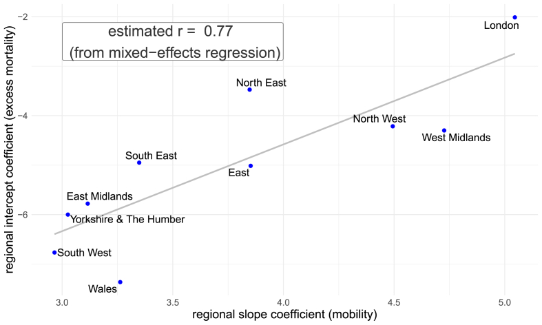
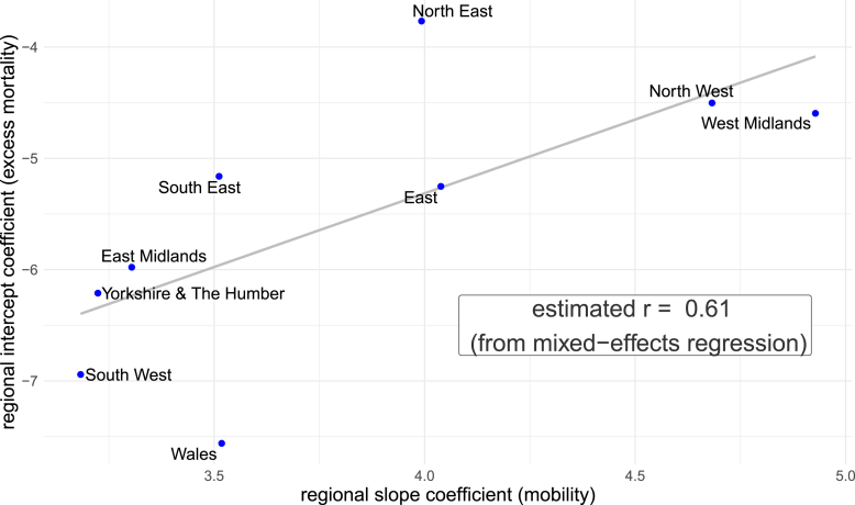
It is important to analyse cross-sectional differences across regions in terms of both excess mortality and response to mobility reductions. The regression model can account for such variations by means of region-specific random intercepts (corresponding to different levels of excess mortality) and random slopes (corresponding to different responses to mobility changes). Focusing on the model with the combined Google index (here and in the remainder of the section), Fig. 3 shows that the intercept and the slope have a positive correlation of 0.77 across the regions, so that those with larger intercepts (i.e. higher excess mortality levels) also have larger slopes (i.e. larger effects of mobility reductions on mortality). The model therefore provides evidence on the degree of regional success of the NPIs, which appear to have had a stronger impact on reducing excess mortality in the regions of London, North West and West Midlands. Differences in the NPIs outcomes may be related to the characteristics of the population (such as population age structure, density, and degree of susceptible individuals) as well as to the extent of behavioural change that occurred within the population.

Fig. 3.

Estimated region-specific intercepts and mobility slopes, as well as their estimated correlation r from the mixed-effects regression in England and Wales by region during weeks 13–33 of 2020. Source: Authors' own elaboration based on data from Office for National Statistics (2021, 2020a) and Google LLC (2021).

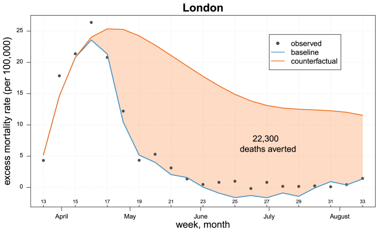
Finally, the estimated model allows us to estimate the number of deaths averted by mobility reductions. This is achieved by simulating a counterfactual worst-case scenario in which mobility is assumed not to have dropped with the introduction of the NPIs but rather to have remained constant at the levels observed before their implementation. The estimated excess mortality rate in the counterfactual scenario is derived from evaluating the mixed-effects regression model under the scenario of no mobility reductions. A graphical illustration of this assumption for the region of London is shown in Fig. A.6 in Appendix A. Table 2 reports the results of this analysis, as well as the estimates of observed excess mortality during the period analysed. The fit of the model and the counterfactual analysis for the region of London are shown in Fig. 4, and the graphs for the remaining nine regions are shown in Fig. A.7of Appendix A. The baseline scenario estimated from the regression model closely follows the observed pattern of the excess mortality rate, which displays a positive reversed U-shape in the weeks 13–20 followed by weeks with values close to zero; the counterfactual analysis displays a similar shape of the excess mortality rate over time, with a considerably slower decrease of the rate resulting from the assumed mobility scenario. The figure shows that the gap between the baseline and counterfactual scenarios widens from week 18: mobility started to strongly decrease in week 13 following the enforcement of the lockdown (see Fig. 2), resulting in a greater difference between observed and assumed (forward) mobility patterns - and thus excess mortality rate. We estimate that about 62,200 excess deaths occurred in England and Wales during the weeks 13–33 of 2020, and that an additional 94,200 excess deaths (95% confidence intervals 86,000–102,100) would have occurred if mobility had not reduced. These absolute estimates display expected significant regional variations, ranging from a minimum of 3600 excess deaths averted in North East to a maximum of 22,300 excess deaths averted in London.

Table 2.

Population size, estimated number of excess deaths, and estimated number of deaths averted by the mobility reductions (counterfactual analysis) with 95% confidence intervals by region in England and Wales during weeks 13–33 of 2020. Estimates have been rounded to the nearest hundredth to avoid giving a false sense of precision in the presence of uncertainty (as in Kontis et al., 2020); as such, figures for the Total row may differ from the sum of the regions. Source: Authors’ own elaboration based on data from Office for National Statistics (2021, 2020a) and Google LLC (2021).

Region	Population (2019)	Estimated excess deaths	Deaths averted (counterfactual)	95% CI
North East	2,669,941	4100	3600	(3300;	4000)
North West	7,341,196	9000	12,700	(11,600;	13,600)
Yorkshire and The Humber	5,502,967	5100	6200	(5600;	7000)
East Midlands	4,835,928	4400	5900	(5300;	6600)
West Midlands	5,934,037	7200	10,700	(9800;	11,500)
East	6,236,072	6300	9600	(8700;	10,400)
London	8,961,989	11,000	22,300	(21,200;	23,300)
South East	9,180,135	9300	12,900	(11,700;	14,100)
South West	5,624,696	3800	6500	(5700;	7300)
Wales	3,152,879	1900	3800	(3300;	4300)
Total	59,439,840	62,200	94,200	(86,000;	102,100)

Fig. 4.

Observed and estimated excess mortality rate (per 100,000 individuals) from the mixed-effects model in the baseline and counterfactual scenarios for the region of London during weeks 13–33 of 2020. Source: Authors' own elaboration based on data from Office for National Statistics (2021, 2020a) and Google LLC (2021).

4. Discussion

Local and national governments around the world have implemented a variety of policies aimed at reducing social contacts to curb the transmission of and deaths from COVID-19. We investigated the relationship between excess mortality and changes in human mobility to assess the effectiveness of non-pharmaceutical interventions. Specifically, we leveraged digital data derived from the Google COVID-19 Community Mobility Reports (Google LLC, 2021) to explore the association between mobility and excess mortality at the regional level in England and Wales.

We found a strong positive relationship between the mobility of Google Maps users and population-level excess mortality, which is considered to be the best indicator of the impact of the pandemic on mortality (National Academies of Sciences, Engineering, and Medicine, 2020). Our analysis determined that a time lag of at least five weeks is needed to reveal a positive association between mobility and mortality, while smaller lags display a negative relationship. A five-week time period is consistent with preliminary estimates of the disease duration from infection to death, with the incubation period (i.e., from infection to symptom onset) that can last up to two weeks (11.5 days with a 95% CI of 8.2–15.6 days (Lauer et al., 2020)), and the course of disease (i.e., from symptom onset to death) that can last up to three weeks (17.8 days with a 95% CI of 16.9–19.2 days (Verity et al., 2020)). This is also consistent with an US-based study, where mobility reductions assessed via mobile phone data were found to anticipate the exponential decay of COVID-deaths by a median of 3–4 weeks (Kogan et al., 2021). Finally, the period of time between infection and death is also related to the individual-level Susceptible-Exposed-Infectious-Recovered (SEIR) compartmental models that have been proposed to describe the spread of COVID-19 (Lin et al., 2020).

Furthermore, our findings are aligned with the existing evidence that mobility restrictions and stay-at-home measures are effective NPIs in the context of a global pandemic (Brauner et al., 2020; Davies et al., 2020; Dehning et al., 2020; Del Fava et al., 2020; Flaxman et al., 2020; Lai et al., 2020). The government's handling of the COVID-19 pandemic in England and Wales has been heavily criticised, particularly given the delayed introduction of NPIs as compared to other countries in Europe (Hale et al., 2020). Nevertheless, the residents of England and Wales appeared to have followed the government guidelines to stay at home when they were issued, as evidenced by: (i) the drastic reduction in mobility of Google Maps users after mid-March, (ii) the large reduction in the daily number of face-to-face contacts per person after the introduction of the physical distancing guidelines (Del Fava et al., 2020; Jarvis et al., 2020), and (iii) the large adoption of social distancing measures and reduction in mobility following the implementation of NPIs as reported through online surveys (Perrotta et al., 2021).

We estimate that about 62,200 excess deaths occurred in England and Wales during weeks 13–33 of 2020 with respect to what was expected from previous years, in line with other findings (Aburto et al., 2021; Office for National Statistics, 2020b). Furthermore, we estimate that an additional 94,200 excess deaths were averted by the reduced mobility following the introduction of the NPIs. The number of lives that could have been saved if earlier and stricter measures had been put in place is unknown, but our results suggest that the potential number of excess deaths could have been much higher in the absence of these interventions. Our results underscore the successful role of NPIs in reducing excess all-cause mortality in the period analysed, mediated by the decrease in mobility. Note that the introduction of governmental measures may have directly or indirectly increased mortality for some specific causes - such as deaths from domestic violence or from limited access to health care. Data on causes of deaths (still not available at the time of writing) will provide insights and comparisons on the effects of NPIs on cause-specific mortality. However, the net effect of the governmental measures on overall mortality appears to have been highly positive.

A limitation of our analysis is that, given the almost simultaneous introduction of different NPIs in March 2020 and the resulting reduction in mobility, we cannot disentangle the individual contribution of each intervention to the change in mobility and mortality. Moreover, the relationship between mobility data and excess mortality is necessarily based on location-based measures, and as such it may be prone to ecological fallacy. Nonetheless, our methodology allows us to isolate and estimate the effect of mobility reductions on excess mortality controlling for (i) the time trend of the epidemic and (ii) all other unobserved region-specific factors, which are allowed for through the random-effect specification of the model.

In our work, we exploit the potential of digital-trace data to estimate human mobility and explain excess mortality, but we are also aware of the shortcomings related to this data source. These are in particular due to the lack of detail concerning the collection and processing of the mobility data. One limitation is that Google does not share absolute numbers in their reports, but only relative changes with respect to the beginning of 2020. Back-engineering the underlying absolute measurements does not seem possible or desirable, given privacy concerns in sparsely populated areas. Moreover, no information is provided on the population composition of Google Maps users, such as age-group or sex breakdowns, thus limiting our ability to assess the representativeness of the data. This lack of detail makes the data less informative than it could possibly be, if all raw measures were made available together with the description of the algorithms used to produce them.

Nonetheless, we believe that the Google mobility data provide a first and valuable approximation to the changes in human mobility occurred during the COVID-19 pandemic. Such data are necessarily affected by biases related to population sampling, which depends on the market share of the operator providing the data and the different usage across socio-demographic groups. However, we are reassured by existing evidence on Internet penetration rates and Google Maps coverage in the UK, and by the high consistency in mobility estimates provided by Google. England and Wales have in fact one of the highest rates of Internet penetration in the world and one of the lowest degrees of gender inequality in Internet access (Garcia et al., 2018). Furthermore, around three quarters of mobile phones worldwide use an Android operating system, on which Google Maps is installed by default (StatCounter, 2020), and survey results indicate that approximately 60% of Android users in the UK have Google Location History reporting enabled (Ruktanonchai et al., 2018). In addition, existing evidence shows very high levels of consistency in mobility estimates obtained from Google and from call detail records (Ruktanonchai et al., 2020). Finally, we are reassured by the similar general patterns of the Google mobility data as compared to other digital sources, such as Apple and Facebook (which only report data for England and Wales as a whole and not at the sub-national level, see Fig. A.8 in Appendix A). Thus, we are confident that this data source approximates well the overall mobility trends at the regional level.

Our study provides evidence on the positive impact of NPIs to mitigate the mortality burden of COVID-19. We conclude by encouraging private companies such as Google to continue sharing data to foster academic research in areas of public interest. Further improvements include more transparency about the data-generating process and the sharing of raw data, keeping as a priority the privacy of users. An increasing number of studies are showing the great potential of digital data for public health research (Coppersmith et al., 2018; Eichstaedt et al., 2018; Oliver et al., 2020; Reece & Danforth, 2017), and the current COVID-19 pandemic further highlights the need for an open conversation on how these data can be used ethically to help save lives.

Ethical statement

The study is based on publicly available data, and as such it did not require ethical approval.

References to the data archives are provided in the manuscript. Moreover, all data and source codes necessary for the reproducibility of our results were stored in the following repository: https://osf.io/4pfb7/.

CRediT author statement

Ugofilippo Basellini: Conceptualization, Methodology, Software, Formal analysis, Data curation, Writing - original draft, Writing - review & editing, Visualization; Diego Alburez-Gutierrez: Methodology, Software, Validation, Writing - original draft, Writing - review & editing; Emanuele Del Fava: Methodology, Validation, Writing - original draft, Writing - review & editing; Daniela Perrotta: Writing - original draft, Writing - review & editing; Marco Bonetti: Methodology, Writing - original draft, Writing - review & editing; Carlo G. Camarda: Methodology, Validation, Writing - original draft, Writing - review & editing; Emilio Zagheni: Conceptualization, Methodology, Writing - original draft, Writing - review & editing.

Declaration of competing interest

The authors declare no competing interests.

Appendix A. Additional Results

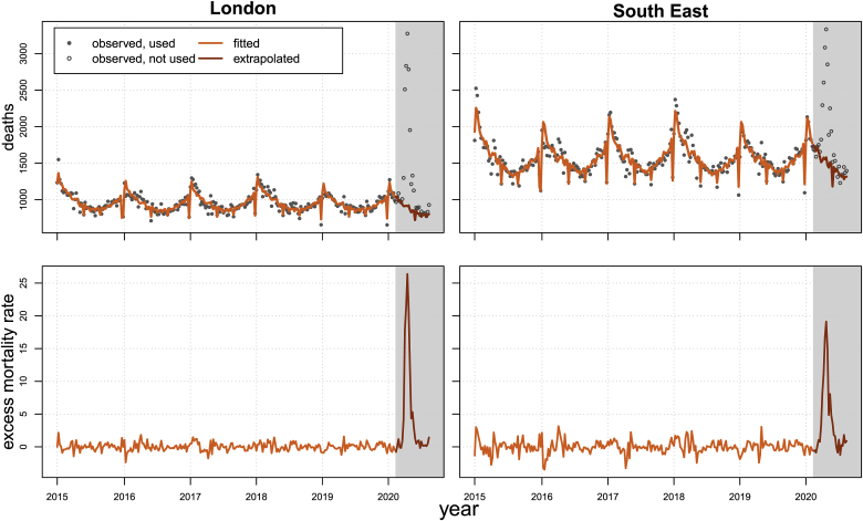
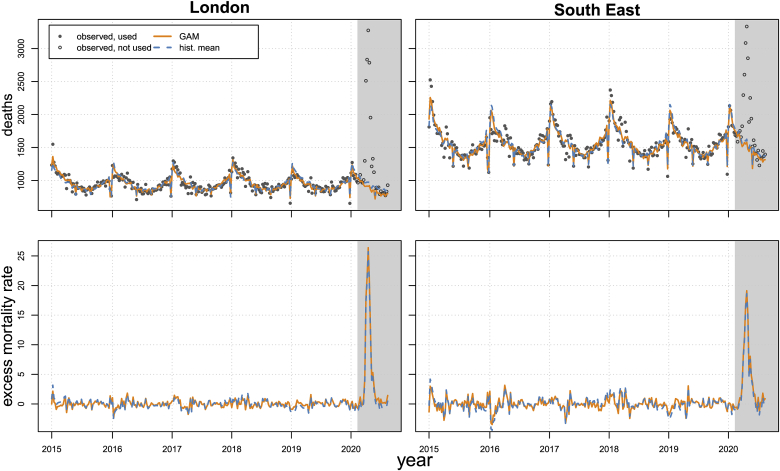
In this Appendix, we report additional results of our analysis. We start by presenting the results of computing the excess mortality rate using the GAM. Fig. A1 shows the results of this approach for two specific regions, London and South East. The grey shaded areas in the panels correspond to the first wave of the COVID-19 pandemic analysed in the paper, and for which corresponding death counts are not employed in the estimation of the GAM. The figure shows that the fitted model captures well the seasonal pattern of the mortality data, as well as the peculiarities of the registration of deaths in some specific weeks (i.e. the lower number of registered deaths during holidays, such as bank holidays and the last week of the year). The lower panels display the excess mortality rate for the two regions: despite being characterised by different absolute numbers of deaths, the regional excess rates have similar values due to different population sizes. Finally, the spike in number of deaths and excess mortality resulting from the COVID-19 pandemic is clearly visible in the period analysed (grey shaded area).

Figure A.1.

Observed (dots) and fitted (lines) weekly number of deaths (upper panels) and excess mortality rate (per 100,000 individuals, lower panels) in the regions of London and South East for the years 2015–2020. The grey shaded area corresponds to the COVID-19 period analysed in the paper. Source: Authors' own elaboration based on data from Office for National Statistics (2021, 2020a).

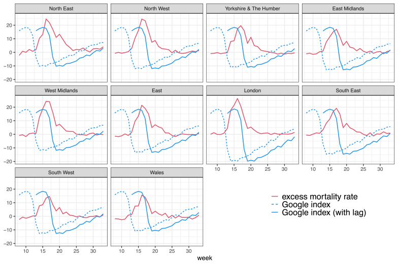
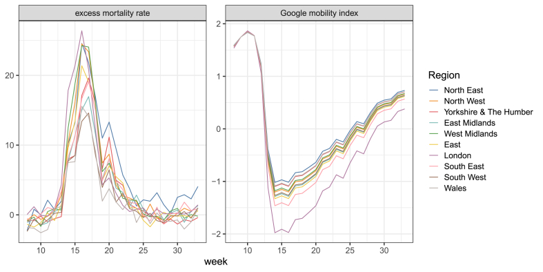
Next, we present the graphs corresponding to Fig. 2 for all the regions analysed in our study. Fig. A.2 shows the time series of the excess mortality rate (per 100,000 individuals) and the change in the Google mobility index for the ten regions of England and Wales during the weeks 8–33 of 2020. In addition, Fig. A.3 shows the time series of the two variables for each of the ten regions side-by-side. Common patterns and regional variations clearly appear from the figure.

Figure A.2.

Time series of excess mortality rate per 100,000 individuals (red lines) and change in Google mobility index in week t (dashed blue lines) and with a five-week forward shift (solid blue lines) in England and Wales by region during weeks 8–33 of 2020. The Google index was multiplied by 10 for illustration purposes. Source: Authors' own elaboration based on data from Office for National Statistics (2021, 2020a) and Google LLC (2021).

Figure A.3.

Time series of excess mortality rate per 100,000 individuals and change in Google mobility index in England and Wales by region during weeks 8–33 of 2020. Source: Authors' own elaboration based on data from Office for National Statistics (2021, 2020a) and Google LLC (2021).

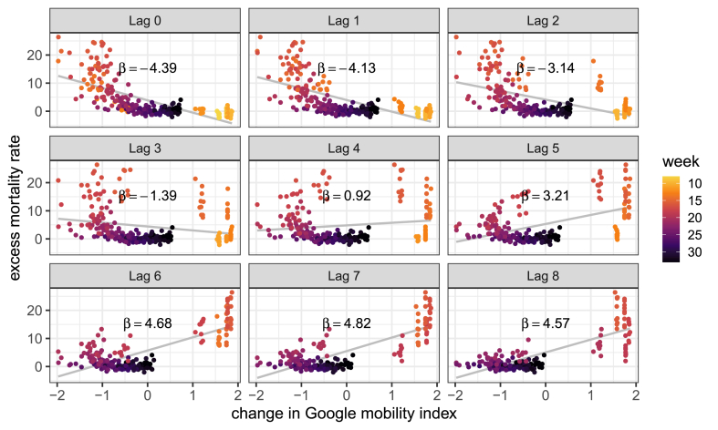
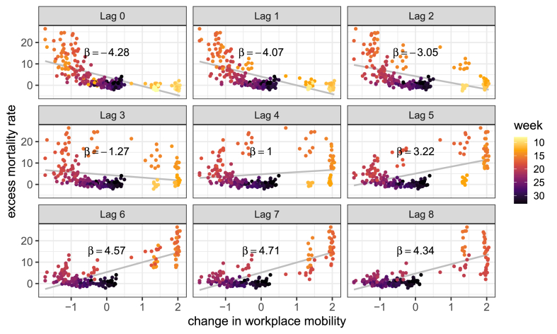
Furthermore, we analyse the relationship between the excess mortality rate and changes in mobility, considering a wide range of possible lags for the latter variable. Figure A.4, Figure A.5 clearly show that the relationship between excess mortality and mobility varies according to the length of time lags. When we consider none or short time lags (between one and three weeks), the relationship between the two variables is negative, i.e., a decrease in mobility is associated with a (future) higher excess mortality. However, for longer time lags (greater or equal to five weeks), we can observe a positive relationship between the two variables, i.e., a decrease in mobility is associated with a (future) lower excess mortality. This holds true for the combined Google mobility index as well as for four categories of the GCMR: grocery, retial, transit and workplaces. For the residential category, the relationship is reversed because time spent at home increased following the implementation of the NPIs (see Fig. 1, main text); for the parks category, the relationship is negative for all lags of time.

Figure A.4.

Linear relationship (with slope equal to β) between excess mortality rate (per 100,000 individuals) and change in the Google mobility index in ten regions of England and Wales during weeks 8–33 of 2020, considering different lags of time for mobility data. Source: Authors' own elaboration based on data from Office for National Statistics (2021, 2020a) and Google LLC (2021).

Figure A.5.

Linear relationship (with slope equal to β) between excess mortality rate (per 100,000 individuals) and (scaled) change in workplace mobility in ten regions of England and Wales during weeks 8–33 of 2020, considering different time lags for mobility data. Source: Authors' own elaboration based on data from Office for National Statistics (2021, 2020a) and Google LLC (2021).

Next, we analyse the role played by different time lags in the relationship between excess mortality and mobility within our regression approach. Table A.1 shows the mixed-effects regression models between excess mortality rate and changes in the Google mobility index occurred 3, 4, 5, 6 and 7 weeks prior. The relationship between excess mortality and mobility changes according to the time lag considered: for shorter time lags (3 and 4 weeks), the two variables have a negative or null association. For time lags of 5 or more weeks, the relationship becomes positive and significant at the 95% confidence level, and the magnitude of the estimated coefficient reduces as the lag increases.

Table A.1.

Estimated coefficients and 95% confidence intervals of linear mixed-effects regression between excess mortality rate (per 100,000 individuals) and changes in Google mobility index occurred x weeks before, using five choices of time lags between the two time series. Note: AIC and BIC values should not be compared here due to different number of observations, and they have been reported for completeness only. Source: Authors' own elaboration based on data from Office for National Statistics (2021, 2020a) and Google LLC (2021).

	Dependent variable: excess mortality rate (per 100,000)
	Linear mixed-effects regression
	3-week lag	4-week lag	5-week lag	6-week lag	7-week lag
Fixed effects
Mobility changes x weeks before	−6.47	−1.27	3.77	2.74	1.26
(95% CI)	(-7.84, −5.10)	(-2.65, 0.12)	(2.71, 4.83)	(1.53, 3.96)	(0.32, 2.21)
Random effects (variance)
Region (intercept)	1.96	1.45	2.67	2.44	1.48
Mobility (slope)	1.06	0.67	0.67	0.96	–
Residual	7.33	7.65	3.38	3.85	7.62
Observations	230	220	210	200	190
Groups	10	10	10	10	10
Log-Likelihood	−560.87	−540.14	−438.36	−428.90	−462.86
AIC	1143.73	1102.27	898.72	879.80	941.71
BIC	1181.55	1139.60	935.54	916.09	967.69

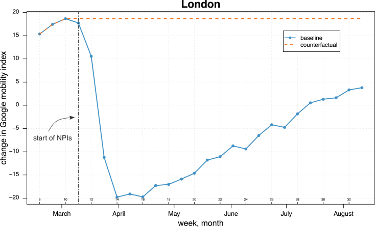
Fig. A.6 shows the underlying mobility assumption of the counterfactual analysis for the region of London. In particular, we assume that mobility did not reduce with the introduction of the NPIs, but that it remained constant at the levels observed before their implementation, i.e. mobility did not change after week 10.

Figure A.6.

Changes in the Google mobility index in the baseline and counterfactual scenarios for the region of London during weeks 8–33 of 2020. Source: Authors' own elaboration based on data from Google LLC (2021).

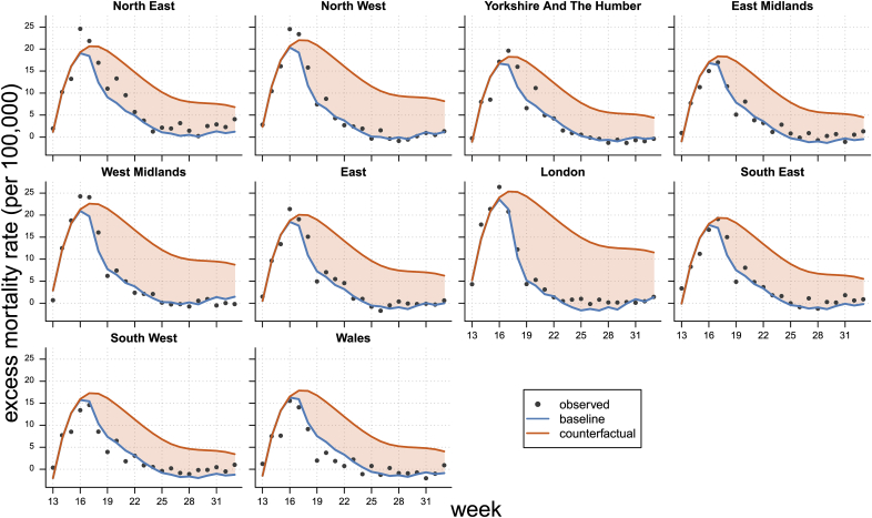
Fig. A.7 shows, for each region analysed, the fit of the estimated mixed-effects regression model as well as the counterfactual analysis which assumes that mobility did not reduce after the introduction of the NPIs.

Figure A.7.

Observed and estimated excess mortality rate (per 100,000 individuals) from the mixed-effects model in the baseline and counterfactual scenarios for the ten regions in England and Wales during weeks 13–33 of 2020. Source: Authors' own elaboration based on data from Office for National Statistics (2021, 2020a) and Google LLC (2021).

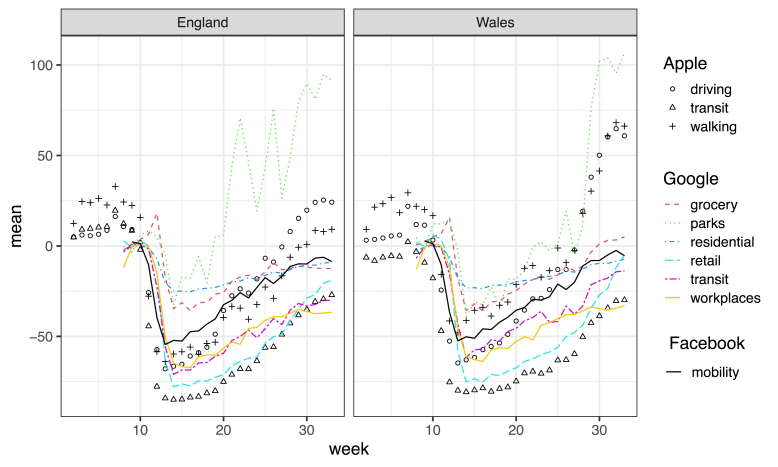
Fig. A.8 compares the GCMR with the mobility data provided by Apple (2020) and Facebook (2020). For the latter two, only country-level data are available for England and Wales (i.e. not at the sub-national level). The figure shows that the six Google categories of mobility indicators are aligned with those of other providers, hence capturing the general mobility patterns throughout England and Wales.

Figure A.8.

Comparison of mobility indicators provided by Apple (categories driving, transit and walking), Facebook (category mobility) and Google (categories residential, workplaces, grocery, transit, retail and parks) for England and Wales in weeks 1–33 of 2020. Note: the sign of the residential category of Google is reversed for illustrative purposes. Source: Authors' own elaboration based on data from Apple (2020), Google LLC (2021) and Facebook (2020).

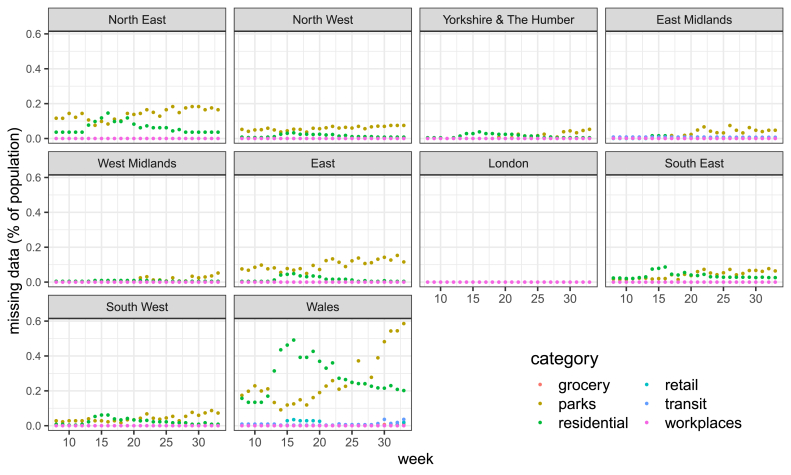
Finally, Fig. A.9 shows the share of the missing data, computed as percentage of the regional population, for the six categories of the Google mobility data by region and week. For most weeks, regions and categories, missing data are relatively low. Only the parks and residential categories, particularly in the Welsh territory, are characterised by some degree of missing data.

Figure A.9.

Share of missing population in the GCMR by region, week and category (residential, workplaces, grocery, transit, retail and parks) for ten regions in England and Wales in weeks 8–33 of 2020. Source: Authors' own elaboration based on data from Google LLC (2021).

Apeendix B. Sensitivity Analysis

In this Appendix, we perform a sensitivity analysis of the results shown in the paper.

B.1 Different estimation of excess mortality

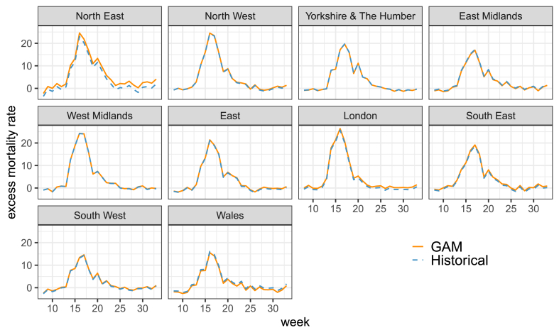
The results shown in our paper are robust to the computation of expected deaths ${\hat{d}}_t$ derived from the GAM. Specifically, we re-run all our analysis using a different estimate of the excess mortality rate. Instead of using the ${\hat{d}}_t$ predicted from the GAM, we computed ${\hat{d}}_t$ for each week in 2020 as the average number of deaths observed in the corresponding weeks between the years 2015–2019. Fig. B.1 shows the estimated numbers of expected deaths and excess mortality rate using the GAM and the historical weekly means of the observed death counts. The excess mortality rates estimated with the two approaches are very similar. In both cases, the decreasing time trend estimated by the GAM predicts a lower number of deaths in the period under study (grey area) as compared to the historical average, resulting in slightly higher excess mortality. Fig. B.2 shows the excess mortality rate obtained with the two approaches for all ten regions of England and Wales during the period analysed.

Figure B.1.

Observed (dots) and fitted (lines) weekly number of deaths (upper panels) and excess mortality rate (per 100,000 individuals, lower panels) using two different approaches (GAM in orange, weekly historical mean in blue) in the regions of London and South East for the years 2015–2020. Source: Authors' own elaboration based on data from Office for National Statistics (2021, 2020a).

Figure B.2.

Excess mortality rate (per 100,000 individuals) computed with two different approaches (GAM in orange, weekly historical mean in blue) in the ten regions of England and Wales during the weeks 8–33 of 2020. Source: Authors' own elaboration based on data from Office for National Statistics (2021, 2020a).

Furthermore, Table B.1 reports the corresponding results of the mixed-effect regression models obtained from using this different computation of the excess mortality rate. Given that the estimates of the excess mortality rates are very similar to those of the GAM, it is not surprising that the results do not change by a great extent when using this alternative computation of excess mortality.

Table B.1.

Estimated coefficients and 95% confidence intervals of linear mixed-effects regression between excess mortality rate (per 100,000 individuals) and changes in mobility occurred five weeks before, measured separately for each model with the combined Google index and the six categories of the GCMR: grocery, workplaces, residential, transit, retail and parks. Note: the excess mortality rate (per 100,000 individuals) is computed from the historical average of weekly deaths instead of the GAM employed in Table 1. Source: Authors' own elaboration based on data from Office for National Statistics (2021, 2020a) and Google LLC (2021).

	Dependent variable: excess mortality rate (per 100,000)
	Linear mixed-effects regression
	Google index	grocery	workplaces	residential	Transit	Retail	parks
Fixed effects
Mobility changes 5 weeks before	3.55	2.57	3.01	−3.24	2.63	3.65	0.63
(95% CI)	(2.54, 4.56)	(1.94, 3.19)	(1.98, 4.03)	(-4.25, −2.23)	(1.64, 3.62)	(2.48, 4.81)	(-0.21, 1.46)
Random effects (variance)
Region (intercept)	1.49	0.50	1.17	1.85	2.11	1.35	0.53
Mobility (slope)	0.66	–	0.85	0.61	0.73	1.22	–
Residual	3.43	4.35	3.64	3.65	3.89	3.55	5.71
Observations	210	210	210	210	210	210	210
Groups	10	10	10	10	10	10	10
Log-Likelihood	−435.42	−452.05	−440.32	−441.53	−448.42	−438.21	−478.91
AIC	892.84	922.09	902.64	905.05	918.85	898.42	975.82
BIC	929.66	952.22	939.46	941.87	955.67	935.23	1005.95

B.2 Other sensitivity analyses

The results shown in our paper are further robust with respect to the number of B-splines employed to describe the time trend of the epidemic. Table B.2 shows the mixed-effects regression models between excess mortality rate and changes in the Google mobility index occurred 5 weeks prior for five different choice of B-spline bases. From the table, it emerges that the estimated mobility coefficient does not change to a great extent, taking values between 3.75 and 5.77 according to different number of bases. Moreover, the estimated coefficient is always statistically significant at the 95% confidence level.

Table B.2.

Estimated coefficients and 95% confidence intervals of linear mixed-effects regression between excess mortality rate (per 100,000 individuals) and changes in Google mobility index occurred five weeks before, using five different choices of B-spline bases for describing the time series of the epidemic. Source: Authors' own elaboration based on data from Office for National Statistics (2021, 2020a) and Google LLC (2021).

	Dependent variable: excess mortality rate (per 100,000)
	Linear mixed-effects regression
	3 B-splines	4 B-splines	5 B-splines	6 B-splines	7 B-splines
Fixed effects
Mobility changes 5 weeks before	5.80	4.24	3.77	5.48	4.81
(95% CI)	(5.05, 6.55)	(3.49, 4.99)	(2.71, 4.83)	(4.38, 6.58)	(3.79, 5.82)
Random effects (variance)
Region (intercept)	3.19	2.81	2.67	3.20	2.99
Mobility (slope)	0.49	0.65	0.67	0.61	0.64
Residual	5.18	3.20	3.38	3.01	2.95
Observations	210	210	210	210	210
Groups	10	10	10	10	10
Log-Likelihood	−481.97	−434.91	−438.36	−427.2	−423.63
AIC	981.94	889.82	898.72	878.4	873.27
BIC	1012.07	923.29	935.54	918.56	916.78

Finally, our results are also robust to the exclusion of the region of London from the analysis. Analysing Fig. A3, London appears as an outlier compared to the other regions since its level of excess mortality and mobility decreased considerably more than in other regions. For this reason, we re-run all our analysis excluding London from the observations employed in our study. Table B.3 shows that the estimated mobility coefficients vary marginally with respect to those estimated in the presence of London, remaining significant at the 95% confidence level. Finally, Fig. B.3 shows that the positive correlation between random slopes and random intercepts in the mixed-effects model reduces only slightly when excluding London from the analysis.

Table B.3.

Estimated coefficients and 95% confidence intervals of linear mixed-effects regression between excess mortality rate (per 100,000 individuals) and changes in mobility occurred five weeks before, measured separately for each model with the combined Google index and the six categories of the GCMR: grocery, workplaces, residential, transit, retail and parks. Note: the region of London was removed from the analysis. Source: Authors' own elaboration based on data from Office for National Statistics (2021, 2020a) and Google LLC (2021).

	Dependent variable: excess mortality rate (per 100,000)
	Linear mixed-effects regression
	Google index	grocery	workplaces	residential	Transit	retail	parks
Fixed effects
Mobility changes 5 weeks before	3.82	2.66	3.07	−3.69	3.10	3.53	0.83
(95% CI)	(2.65, 4.99)	(1.92, 3.39)	(1.91, 4.22)	(-4.94, −2.45)	(1.94, 4.27)	(2.37, 4.68)	(-0.01, 1.67)
Random effects (variance)
Region (intercept)	1.66	1.46	1.48	1.51	1.79	1.70	1.55
Mobility (slope)	0.52	0.51	0.52	0.48	0.38	0.56	–
Residual	3.56	3.11	3.82	3.79	3.94	3.64	4.97
Observations	189	189	189	189	189	189	189
Groups	9	9	9	9	9	9	9
Log-Likelihood	−396.24	−384.79	−402.24	−400.56	−404.75	−398.25	−420.92
AIC	814.48	791.57	826.48	823.12	831.5	818.51	859.83
BIC	850.14	827.23	862.14	858.78	867.16	854.17	889.01

Fig. B.3.

Estimated region-specific intercepts and mobility coefficients, as well as their estimated correlation r from the mixed-effects regression in nine regions of England and Wales (excluding London) during weeks 13–33 of 2020. Source: Authors' own elaboration based on data from Office for National Statistics (2021, 2020a) and Google LLC (2021).

References

- Aburto J.M., Kashyap R., Schöley J., Angus C., Ermisch J., Mills M.C., Dowd J.B. Estimating the burden of the COVID-19 pandemic on mortality, life expectancy and lifespan inequality in england and Wales: A population-level analysis. Journal of Epidemiology & Community Health. 2021 doi: 10.1136/jech-2020-215505. [DOI] [PMC free article] [PubMed] [Google Scholar]
- Apple COVID-19 - mobility trends reports. 2020. https://covid19.apple.com/mobility Available at:
- Badr H.S., Du H., Marshall M., Dong E., Squire M.M., Gardner L.M. Association between mobility patterns and COVID-19 transmission in the USA: A mathematical modelling study. The Lancet Infectious Diseases. 2020;20(11):1247–1254. doi: 10.1016/S1473-3099(20)30553-3. [DOI] [PMC free article] [PubMed] [Google Scholar]
- Bates D., Mächler M., Bolker B., Walker S. Fitting linear mixed-effects models using lme4. Journal of Statistical Software. 2015;67(1):1–48. [Google Scholar]
- Brauner J.M., Mindermann S., Sharma M., Johnston D., Salvatier J., Gavenčiak T.…Kulveit J. Inferring the effectiveness of government interventions against COVID-19. Science. 2020;371(6531) doi: 10.1126/science.abd9338. [DOI] [PMC free article] [PubMed] [Google Scholar]
- Buss L.F., Prete C.A., Abrahim C.M.M., Mendrone A., Salomon T., de Almeida-Neto C., França R.F.O., Belotti M.C., Carvalho M.P.S.S., Costa A.G., Crispim M.A.E., Ferreira S.C., Fraiji N.A., Gurzenda S., Whittaker C., Kamaura L.T., Takecian P.L., da Silva Peixoto P., Oikawa M.K.…Sabino E.C. Three-quarters attack rate of SARS-CoV-2 in the Brazilian Amazon during a largely unmitigated epidemic. Science. 2021;371(6526):288–292. doi: 10.1126/science.abe9728. [DOI] [PMC free article] [PubMed] [Google Scholar]
- Cameron-Blake E., Tatlow H., Wood A., Hale T., Kira B., Petherick A., Phillips T. 2020. Variation in the response to COVID-19 across the four nations of the United Kingdom.https://www.bsg.ox.ac.uk/research/publications/variation-response-covid-19-across-four-nations-united-kingdom Blavatnik School of Government Working Paper. October 26, 2020. Available at: [Google Scholar]
- Coppersmith G., Leary R., Crutchley P., Fine A. Natural language processing of social media as screening for suicide risk. Biomedical Informatics Insights. 2018;10 doi: 10.1177/1178222618792860. [DOI] [PMC free article] [PubMed] [Google Scholar]
- Davies N.G., Barnard R.C., Jarvis C.I., Russell T.W., Semple M.G., Jit M., Edmunds W.J. The lancet infectious diseases. 2020. Association of tiered restrictions and a second lockdown with COVID-19 deaths and hospital admissions in england: A modelling study. [DOI] [PMC free article] [PubMed] [Google Scholar]
- Dehning J., Zierenberg J., Spitzner F.P., Wibral M., Neto J.P., Wilczek M., Priesemann V. Inferring change points in the spread of COVID-19 reveals the effectiveness of interventions. Science. 2020;369(6500) doi: 10.1126/science.abb9789. [DOI] [PMC free article] [PubMed] [Google Scholar]
- Del Fava E., Cimentada J., Perrotta D., Grow A., Rampazzo F., Gil-Clavel S., Zagheni E. 2020. The differential impact of physical distancing strategies on social contacts relevant for the spread of COVID-19. medRxiv. [DOI] [PMC free article] [PubMed] [Google Scholar]
- Drake T.M., Docherty A.B., Weiser T.G., Yule S., Sheikh A., Harrison E.M. The effects of physical distancing on population mobility during the COVID-19 pandemic in the UK. The Lancet Digital Health. 2020;2(8):E385–E387. doi: 10.1016/S2589-7500(20)30134-5. [DOI] [PMC free article] [PubMed] [Google Scholar]
- Eichstaedt J.C., Smith R.J., Merchant R.M., Ungar L.H., Crutchley P., Preoţiuc-Pietro D., Asch D.A., Schwartz H.A. Facebook language predicts depression in medical records. Proceedings of the National Academy of Sciences. 2018;115(44):11203–11208. doi: 10.1073/pnas.1802331115. [DOI] [PMC free article] [PubMed] [Google Scholar]
- Facebook Movement range Maps. 2020. https://data.humdata.org/dataset/movement-range-maps Available at:
- Flaxman S., Mishra S., Gandy A., Unwin H.J.T., Mellan T.A., Coupland H.…Bhatt S. Estimating the effects of non-pharmaceutical interventions on COVID-19 in Europe. Nature. 2020;584:257–261. doi: 10.1038/s41586-020-2405-7. [DOI] [PubMed] [Google Scholar]
- Garcia D., Mitike Kassa Y., Cuevas A., Cebrian M., Moro E., Rahwan I., Cuevas R. Analyzing gender inequality through large-scale Facebook advertising data. Proceedings of the National Academy of Sciences. 2018;115(27):6958–6963. doi: 10.1073/pnas.1717781115. https://www.pnas.org/content/115/27/6958.full.pdf Publisher: National Academy of Sciences eprint: [DOI] [PMC free article] [PubMed] [Google Scholar]
- Google L.L.C. Google COVID-19 community mobility reports. 2021. https://www.google.com/covid19/mobility/ Available at:
- Hale T., Angrist N., Kira B., Petherick A., Phillips T., Webster S. 2020. Variation in government responses to COVID-19.www.bsg.ox.ac.uk/covidtracker Blavatnik School of Government Working Paper. May 25, 2020. Available at: [DOI] [PMC free article] [PubMed] [Google Scholar]
- Havers F.P., Reed C., Lim T., Montgomery J.M., Klena J.D., Hall A.J., Fry A.M., Cannon D.L., Chiang C.-F., Gibbons A., Krapiunaya I., Morales-Betoulle M., Roguski K., Rasheed M.A.U., Freeman B., Lester S., Mills L., Carroll D.S., Owen S.M.…Thornburg N.J. Seroprevalence of antibodies to SARS-CoV-2 in 10 sites in the United States, march 23-may 12, 2020. JAMA Internal Medicine. 2020;180(12):1576. doi: 10.1001/jamainternmed.2020.4130. [DOI] [PMC free article] [PubMed] [Google Scholar]
- Hsiang S., Allen D., Annan-Phan S., Bell K., Bolliger I., Chong T., Druckenmiller H., Huang L.Y., Hultgren A., Krasovich E., Lau P., Lee J., Rolf E., Tseng J., Wu T. The effect of large-scale anti-contagion policies on the COVID-19 pandemic. Nature. 2020;584(7820):262–267. doi: 10.1038/s41586-020-2404-8. [DOI] [PubMed] [Google Scholar]
- Jarvis C.I., Van Zandvoort K., Gimma A., Prem K., working group C.C.-., Klepac P., Rubin G.J., Edmunds W.J. Quantifying the impact of physical distance measures on the transmission of COVID-19 in the UK. BMC Medicine. 2020;18 doi: 10.1186/s12916-020-01597-8. [DOI] [PMC free article] [PubMed] [Google Scholar]
- Kogan N.E., Clemente L., Liautaud P., Kaashoek J., Link N.B., Nguyen A.T., Lu F.S., Huybers P., Resch B., Havas C., Petutschnig A., Davis J., Chinazzi M., Mustafa B., Hanage W.P., Vespignani A., Santillana M. An early warning approach to monitor COVID-19 activity with multiple digital traces in near real time. Science Advances. 2021;7(10) doi: 10.1126/sciadv.abd6989. [DOI] [PMC free article] [PubMed] [Google Scholar]
- Kontis V., Bennett J.E., Rashid T., Parks R.M., Pearson-Stuttard J., Guillot M., Asaria P., Zhou B., Battaglini M., Corsetti G., McKee M., Cesare M.D., Mathers C.D., Ezzati M. Magnitude, demographics and dynamics of the effect of the first wave of the COVID-19 pandemic on all-cause mortality in 21 industrialized countries. Nature Medicine. 2020;26(12):1919–1928. doi: 10.1038/s41591-020-1112-0. [DOI] [PMC free article] [PubMed] [Google Scholar]
- Kupferschmidt K. Europe is locking down again—but its strategy is unclear. Science. 2020;370(6517):644–645. doi: 10.1126/science.370.6517.644. [DOI] [PubMed] [Google Scholar]
- Lai S., Ruktanonchai N.W., Zhou L., Prosper O., Luo W., Floyd J.R.…Tatem A.J. Effect of non-pharmaceutical interventions to contain COVID-19 in China. Nature. 2020;585:410–413. doi: 10.1038/s41586-020-2293-x. [DOI] [PMC free article] [PubMed] [Google Scholar]
- Lauer S.A., Grantz K.H., Bi Q., Jones F.K., Zheng Q., Meredith H.R., Azman A.S., Reich N.G., Lessler J. The incubation period of coronavirus disease 2019 (COVID-19) from publicly reported confirmed cases: Estimation and application. Annals of Internal Medicine. 2020;172(9):577–582. doi: 10.7326/M20-0504. [DOI] [PMC free article] [PubMed] [Google Scholar]
- Li J., Bien J., Wells M.T. rTensor: An R package for multidimensional array (tensor) unfolding, multiplication, and decomposition. Journal of Statistical Software. 2018;87(10):1–31. [Google Scholar]
- Lin Q., Zhao S., Gao D., Lou Y., Yang S., Musa S.S., Wang M.H., Cai Y., Wang W., Yang L., He D. A conceptual model for the coronavirus disease 2019 (COVID-19) outbreak in Wuhan, China with individual reaction and governmental action. International Journal of Infectious Diseases. 2020;93:211–216. doi: 10.1016/j.ijid.2020.02.058. [DOI] [PMC free article] [PubMed] [Google Scholar]
- Lu H., Plataniotis K., Venetsanopoulos A. Mpca: Multilinear principal component analysis of tensor objects. IEEE Transactions on Neural Networks. 2008;19(1):18–39. doi: 10.1109/TNN.2007.901277. [DOI] [PubMed] [Google Scholar]
- National Academies of Sciences, Engineering, and Medicine . The National Academies Press; Washington, DC: 2020. Evaluating data types: A guide for decision makers using data to understand the extent and spread of COVID-19. [Google Scholar]
- Office for National Statistics Estimates of the population for the UK, england and Wales, scotland and northern Ireland. 2020. https://www.ons.gov.uk/peoplepopulationandcommunity/populationandmigration/populationestimates/datasets/populationestimatesforukenglandandwalesscotlandandnorthernireland Available at:
- Office for National Statistics Statistical bulletin: Deaths registered weekly in england and Wales, provisional: Week ending 14 August 2020. 2020. https://www.ons.gov.uk/peoplepopulationandcommunity/birthsdeathsandmarriages/deaths/bulletins/deathsregisteredweeklyinenglandandwalesprovisional/weekending14august2020 Available at:
- Office for National Statistics Deaths registered weekly in England and Wales, provisional. 2021. Available at: https://www.ons.gov.uk/peoplepopulationandcommunity/birthsdeathsandmarriages/deaths/datasets/weeklyprovisionalfiguresondeathsregisteredinenglandandwales.
- Oliver N., Lepri B., Sterly H., Lambiotte R., Deletaille S., Nadai M.D., Letouzé E., Salah A.A., Benjamins R., Cattuto C., Colizza V., Cordes N.d., Fraiberger S.P., Koebe T., Lehmann S., Murillo J., Pentland A., Pham P.N., Pivetta F.…Vinck P. Mobile phone data for informing public health actions across the COVID-19 pandemic life cycle. Science Advances. 2020;6 doi: 10.1126/sciadv.abc0764. [DOI] [PMC free article] [PubMed] [Google Scholar]
- Pepe E., Bajardi P., Gauvin L., Privitera F., Lake B., Cattuto C., Tizzoni M. COVID-19 outbreak response, a dataset to assess mobility changes in Italy following national lockdown. Scientific Data. 2020;7(1):230. doi: 10.1038/s41597-020-00575-2. [DOI] [PMC free article] [PubMed] [Google Scholar]
- Perrotta D., Grow A., Rampazzo F., Cimentada J., Del Fava E., Gil-Clavel S., Zagheni E. Behaviours and attitudes in response to the COVID-19 pandemic: insights from a cross-national Facebook survey. EPJ Data Science. 2021;10 doi: 10.1140/epjds/s13688-021-00270-1. [DOI] [PMC free article] [PubMed] [Google Scholar]
- Pullano G., Domenico L.D., Sabbatini C.E., Valdano E., Turbelin C., Debin M.…Colizza V. Underdetection of cases of COVID-19 in France threatens epidemic control. Nature. 2021;590:134–139. doi: 10.1038/s41586-020-03095-6. [DOI] [PubMed] [Google Scholar]
- R Development Core Team . R Foundation for Statistical Computing; Vienna, Austria: 2020. R: A language and environment for statistical computing. [Google Scholar]
- Rau R. Springer; Berlin, Heidelberg: 2007. Seasonality in human mortality. [Google Scholar]
- Reece A.G., Danforth C.M. Instagram photos reveal predictive markers of depression. EPJ Data Science. 2017;6(1):1–12. [Google Scholar]
- Riley S. Large-scale spatial-transmission models of infectious disease. Science. 2007;316(5829):1298–1301. doi: 10.1126/science.1134695. [DOI] [PubMed] [Google Scholar]
- Ruktanonchai N.W., Floyd J., Lai S., Ruktanonchai C.W., Sadilek A., Rente-Lourenco P.…Steele J. Assessing the impact of coordinated COVID-19 exit strategies across Europe. Science. 2020;369(6510):1465–1470. doi: 10.1126/science.abc5096. [DOI] [PMC free article] [PubMed] [Google Scholar]
- Ruktanonchai N.W., Ruktanonchai C.W., Floyd J.R., Tatem A.J. Using Google Location History data to quantify fine-scale human mobility. International Journal of Health Geographics. 2018;17(1):28. doi: 10.1186/s12942-018-0150-z. [DOI] [PMC free article] [PubMed] [Google Scholar]
- Schlosser F., Maier B.F., Jack O., Hinrichs D., Zachariae A., Brockmann D. COVID-19 lockdown induces disease-mitigating structural changes in mobility networks. Proceedings of the National Academy of Sciences. 2020;117(52):32883–32890. doi: 10.1073/pnas.2012326117. [DOI] [PMC free article] [PubMed] [Google Scholar]
- StatCounter . 2020. Mobile operating systems' market share worldwide from January 2012 to December 2019. Statista.https://www.statista.com/statistics/272698/global-market-share-held-by-mobile-operating-systems-since-2009/ Retrieved July 24, 2020. Available at: [Google Scholar]
- Tatem A.J., Rogers D.J., Hay S.I. Global transport networks and infectious disease spread. Advances in Parasitology. 2006;62:293–343. doi: 10.1016/S0065-308X(05)62009-X. [DOI] [PMC free article] [PubMed] [Google Scholar]
- Verity R., Okell L.C., Dorigatti I., Winskill P., Whittaker C., Imai N., Cuomo-Dannenburg G., Thompson H., Walker P.G.T., Fu H., Dighe A., Griffin J.T., Baguelin M., Bhatia S., Boonyasiri A., Cori A., Cucunubá Z., FitzJohn R., Gaythorpe K.…Ferguson N.M. Estimates of the severity of coronavirus disease 2019: A model-based analysis. The Lancet Infectious Diseases. 2020;20(6):669–677. doi: 10.1016/S1473-3099(20)30243-7. [DOI] [PMC free article] [PubMed] [Google Scholar]
- Wesolowski A., Buckee C.O., Engø-Monsen K., Metcalf C.J.E. Connecting mobility to infectious diseases: The promise and limits of mobile phone data. The Journal of Infectious Diseases. 2016;214(suppl_4):S414–S420. doi: 10.1093/infdis/jiw273. [DOI] [PMC free article] [PubMed] [Google Scholar]
- Wilson M.E. Travel and the emergence of infectious diseases. Emerging Infectious Diseases. 1995;1(2):39. doi: 10.3201/eid0102.950201. [DOI] [PMC free article] [PubMed] [Google Scholar]
- Wood S.N. 2019. mgcv: Mixed GAM computation Vehicle with GCV/AIC/REML smoothness estimation. R package version 1. [Google Scholar]
- World Health Organization . -; 2021. Coronavirus disease 2019 (COVID-19): Weekly epidemiological update.https://www.who.int/emergencies/diseases/novel-coronavirus-2019/situation-reports 2 February 2021. [Google Scholar]
- Zhang J., Litvinova M., Liang Y., Wang Y., Wang W., Zhao S.…Yu H. Changes in contact patterns shape the dynamics of the COVID-19 outbreak in China. Science. 2020;368(6498):1481–1486. doi: 10.1126/science.abb8001. [DOI] [PMC free article] [PubMed] [Google Scholar]