Cross-modality deep learning: Contouring of MRI data from annotated CT data only

Abstract

Purpose:

Online adaptive radiotherapy would greatly benefit from the development of reliable autosegmentation algorithms for organs-at-risk and radiation targets. Current practice of manual segmentation is subjective and time-consuming. While deep learning-based algorithms offer ample opportunities to solve this problem, they typically require large datasets. However, medical imaging data are generally sparse, in particular annotated MR images for radiotherapy. In this study, we developed a method to exploit the wealth of publicly available, annotated CT images to generate synthetic MR images, which could then be used to train a convolutional neural network (CNN) to segment the parotid glands on MR images of head and neck cancer patients.

Methods:

Imaging data comprised 202 annotated CT and 27 annotated MR images. The unpaired CT and MR images were fed into a 2D CycleGAN network to generate synthetic MR images from the CT images. Annotations of axial slices of the synthetic images were generated by propagating the CT contours. These were then used to train a 2D CNN. We assessed the segmentation accuracy using the real MR images as test dataset. The accuracy was quantified with the 3D Dice similarity coefficient (DSC), Hausdorff distance (HD), and mean surface distance (MSD) between manual and auto-generated contours. We benchmarked the approach by a comparison to the interobserver variation determined for the real MR images, as well as to the accuracy when training the 2D CNN to segment the CT images.

Results:

The determined accuracy (DSC: 0.77±0.07, HD: 18.04±12.59mm, MSD: 2.51±1.47mm) was close to the interobserver variation (DSC: 0.84±0.06, HD: 10.85±5.74mm, MSD: 1.50 ±0.77mm), as well as to the accuracy when training the 2D CNN to segment the CT images (DSC: 0.81 ±0.07, HD: 13.00±7.61mm, MSD: 1.87±0.84mm).

Conclusions:

The introduced cross-modality learning technique can be of great value for segmentation problems with sparse training data. We anticipate using this method with any nonannotated MRI dataset to generate annotated synthetic MR images of the same type via image style transfer from annotated CT images. Furthermore, as this technique allows for fast adaptation of annotated datasets from one imaging modality to another, it could prove useful for translating between large varieties of MRI contrasts due to differences in imaging protocols within and between institutions.

1. INTRODUCTION

Radiotherapy (RT) requires accurate segmentation of irradiation targets and organs at risk (OARs) to be able to plan and deliver a sufficient dose to the targets while minimizing side effects to the OARs. Current practice of manual segmentation is subjective and time-consuming,^1,2 in particular for the treatment of head and neck cancer (HNC) patients due to the complex anatomy, including many OARs and irradiation targets associated with HNC. Automating the outlining of regions of interest (ROIs) would allow to alleviate the enormous workload of manual segmentation and reduce inter- and intraobserver variabilities.³

New methodologies based on deep learning offer ample opportunities to solve this problem, of which deep convolutional neural networks (CNNs)⁴ are particularly promising. CNNs are supervised approaches that require annotated training images. Recently, CNNs have successfully been implemented to contour OARs on HNC CT images.^5–9 The success of CNNs on CT images can strongly be attributed to the large amounts of available annotated data, as CT is being used on daily base in most RT clinics throughout the world. While it is still unclear how many training examples deep learning-based algorithms need, it is evident that the generalizability increases with an increasing diversity in the training data.

However, for less common imaging techniques that are only starting to be used in clinical routine for radiotherapy, such as ultrasound,¹⁰ positron emission tomography (PET),^11,12 and magnetic resonance imaging (MRI),^13–16 annotated data are rare. Furthermore, MRI contrast varies a lot depending on sequence settings, causing limited transfer-ability onto a new dataset with new MRI settings. Despite the limited ground truth data, these novel techniques can greatly gain from automatic contouring, particularly when these imaging techniques are to be applied daily.^17–22 In this study, we exploited the large amount of annotated CT datasets to enrich the MRI datasets which have limited or no annotated data.

A common approach to tackle the lack of training data is to augment them with random rotations, translations, geometric scaling, mirroring, contrast stretching, or elastic deformations.^23,24 While these methods try to increase the diversity in the training data, they are generally not able to mimic the large variabilities existing in the full population of patients’ anatomies. Another approach is to use pretrained networks on related problems via transfer learning.²⁵ Instead of training a model from scratch, weights from a model, which was trained for another, typically much larger dataset and task, can be used to improve generalization and robustness. Most published studies use transfer learning by starting from pretrained classification models on natural images.^26,27 However, data augmentation and transfer learning require that the ground truth segmentation needs to be repeated for every novel MR contrast setting. Moreover, these methods face the challenge to be able to reflect a broad range of patients’ anatomies.

Recently, deep learning has been used for synthetic image generation.²⁸ Especially promising are generative adversarial networks (GANs) which can learn to mimic any data distribution and have been applied to image-to-image translation problems, such as reconstructing objects from edge maps.²⁹ In the field of medical image segmentation, GANs were lately employed for data augmentation purposes.^30,31 Conventional GANs require paired datasets as their input, which in practice may be hard to obtain for medical imaging and would limit the dataset to patients who were imaged with multiple imaging modalities. An extension of GANs to unpaired datasets is the CycleGAN.³² Such a network was, for example, used to generate paintings from photographs, which would be infeasible if matched images were required. In a radiotherapy context, the CycleGAN was used to generate synthetic CT images from unmatched brain MR data³³ for MR-only treatment planning purposes.

In this study, we used a CycleGAN to generate synthetic MR images from CT images of a different patient cohort. Instead of using the synthetic images for data augmentation, we took one step further and trained a 2D CNN solely based on the synthetic images to segment the parotid glands. This resembled the situation where one would like to employ annotated data from a different imaging domain (here CT images) for a new imaging domain (here MR images) to avoid the need for the time-consuming and expensive manual segmentation process. Furthermore, the CycleGAN method allows for the datasets to be unpaired. To the best of our knowledge, this was the first study to generate synthetic MR images from CT images for the purpose of training a network to segment MR images.

2. MATERIALS AND METHODS

All data processing was done in Python (version 3.6). Neural networks were trained using Pytorch (version 0.4.1), Tensorflow (version 1.10.0), and Keras (version 2.2.2).

2.A. Data acquisition and preparation

The imaging database comprised 202 annotated CT images and 27 annotated MR images of two different patient cohorts. The MR library contained baseline T2-weighted MR scans of 27 patients, all with a tumor at the base of the tongue and treated with RT at the MD Anderson Cancer Center (Houston, Texas, USA). One clinician at the Royal Marsden Hospital (London, UK) manually delineated the left and right parotid glands using the treatment planning system Raystation (Raysearch, Stockholm, Sweden). The CT images from the publicly available database of the Cancer Imaging Archive,³⁴ as well as the MICCAI HNC segmentation challenge³⁵ served as additional input data for the image synthesis method. Figure 1 demonstrates exemplary axial, sagittal and coronal views of all imaging modalities, together with the manually segmented ROIs. Table I lists the relevant image acquisition parameters for each imaging modality of the original database.

Fig 1.

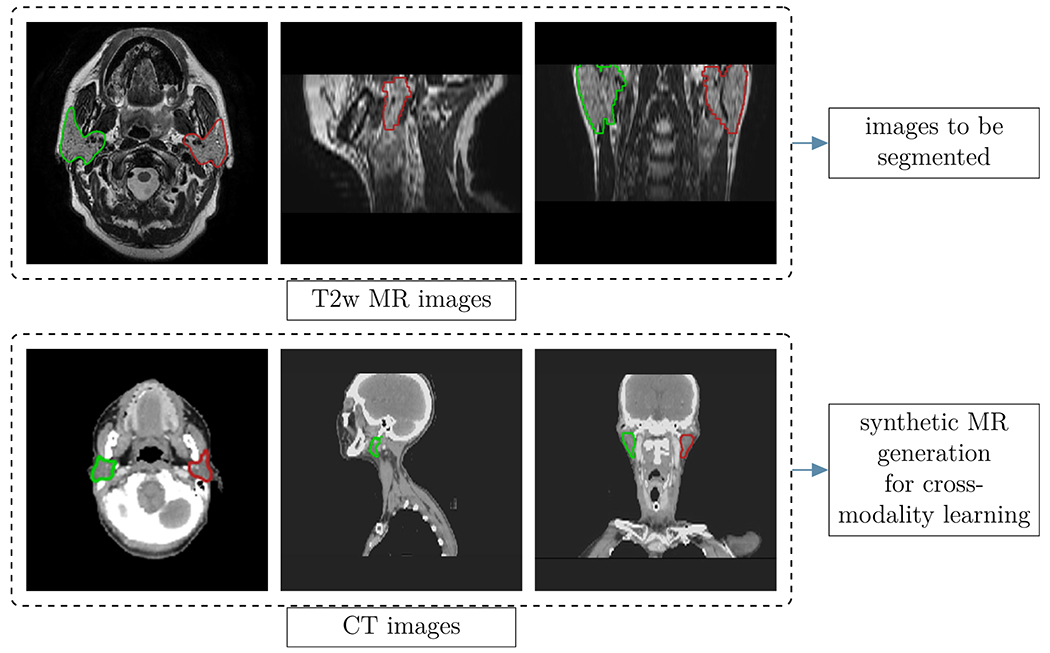
Examples of images used in this study: Axial, coronal and sagittal views of the T2w MR (top row) and the CT images (bottom row). The colored regions represent the manually segmented regions of interest of the left (red) and right (green) parotids. The CT images were downloaded from the publicly available database of the Cancer Imaging Archive,³⁴ as well as the MICCAI head and neck cancer segmentation challenge.³⁵

Table I.

Imaging parameters of the main, unprocessed database (T2-weighted MR and CT images).

Parameter	T2w MR	CT
FOV [#pixels]	512×512	512×512
#slices	30	[165, 235]
Voxel size [mm3]	0.5×0.5×4	0.98×0.98×2.5
TE [ms]	[96.72, 107.30]	n.a.
TR [ms]	[3198, 4000]	n.a.
Flip angle [°]	90	n.a.
Sequence type	2D T2w spin echo	n.a.
Field strength/tube voltage	3 T	120 keV

As the resolution and field of view of the MR and CT images were different from each other, we developed an automated pipeline to ensure that CT and MR images had a similar resolution and field of view. Both CT and MR images were resampled to a 1×1 mm² in-plane resolution. The CT images were cropped to a window of 256×256 pixels in-plane, centered around the head, which was obtained by detecting the skull outline. In the cranial-caudal direction, the range of the CT images was manually restricted to be similar to that of the MR images. Resampling along the cranial-caudal direction was not necessary as the applied method was a 2D method and input was unpaired for the CycleGAN.

As image intensities can vary between MR images, we standardized the contrast with an intensity histogram-based thresholding technique, before feeding them into the network. We rescaled the intensities in the CT images to the recommended soft-tissue window (level 40, window 350 HU)³⁶ to increase visibility of the parotid glands. Additionally, intensities of both imaging modalities were mapped to an intensity range between 0 and 255.

2.B. Overview of employed method

Figure 2 provides an overview of the method employed in this study. It consisted of three steps:

Fig 2.

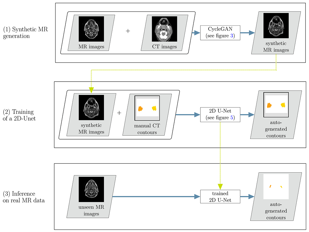
Overview of the proposed cross-modality learning method: in the first step (top row), synthetic MR images are generated through the CycleGAN network. The synthetic MR images are then fed into a 2D U-Net, together with the annotations from the CT images (second row). In a third step, the trained network is applied to unseen real MR images (bottom row)

1. For each axial slice of the CT images, a corresponding^* synthetic MR axial slice was generated using the 2D CycleGAN (see Section 2.C.).

2. A 2D U-Net was trained using the synthetic MR images and corresponding manual contours from CT images as input (see Section 2.E.).

3. The trained 2D U-Net was used to propose contours on unseen real MR images (see Section 2.G).

2.C. Synthetic MR generation

Step (1) of the workflow illustrated in Fig. 2 comprised the synthetic MR generation. The unpaired 2D slices from the CT and MR images were fed into a 2D CycleGAN network to generate synthetic MR images for each of the 202 CT images. We used the PyTorch³⁷ implementation provided by Zhu et al.³² on Github.^† In the following paragraphs, we shortly describe the CycleGAN and the adjustments we made to the PyTorch implementation. For further details, we refer to the original implementation and publication.³²

2.C.1. General workflow and objectives

The CycleGAN consists of two basic networks: a generator and a discriminator network. In our case, the generator’s task was to generate realistic examples of MR images from a given CT image, while the discriminator’s task was to classify presented examples as real or fake. These two networks compete in an adversarial game of which the aim is to improve each other’s performance. While this method can generate images which appear to be realistic, nothing ensures a corresponding anatomy between the input CT image and the generated synthetic MR image.

To reduce the space of possible mappings, CycleGANs employ a cycle-consistency strategy.³² This is achieved by introducing two additional networks, a generator that is trained to generate CT images from MR images and a discriminator that learns to distinguish real from fake CT images. Cycle-consistency loss functions then guarantee that reconstructed CT images which have gone through the full cycle (CT->MR->CT) are similar to the original CT images and vice versa for MR images. Figure 3 illustrates these forward (CT→MR→CT) and backward cycles (MR→CT→MR).

Fig 3.

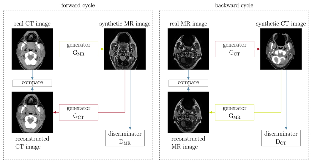
Illustration of the CycleGAN method: two cycles are introduced such that the generated synthetic images resemble the input images (Cycle for synthetic MR images on the left and for synthetic CT images on the right). The different networks are illustrated in detail in Fig. 4.

To further constrain the generated synthetic MR images to ones that geometrically match the source CT images, we introduced a geometric consistency loss as additional contribution to the objective function. For this purpose, we determined the skull mask of the source CT and the synthetic MR and calculated the binary cross-entropy between these masks. We introduced the same loss for the mapping in the opposite direction (source MR to synthetic CT). With M(I_CT) denoting the skull mask of a CT image I_CT and G_MR representing the generator which generates MR images from CT images, the geometric loss term ℒ_geo,CT for the forward cycle yields

$$\begin{array}{l}{ℒ}_{\text{geo,CT}}\left(G_{\text{MR}},I_{\text{CT}}\right)=M\left(G_{\text{MR}}\left(I_{\text{CT}}\right)\right)\cdot \text{log}\left(M\left(I_{\text{CT}}\right)\right)\\ +\left(1-M\left(G_{\text{MR}}\left(I_{\text{CT}}\right)\right)\right)\cdot \text{log}\left(1-M\left(I_{\text{CT}}\right)\right).\end{array}$$ (1)

The geometric loss term for the backward cycle can be obtained by replacing the MR by the CT and vice versa. This loss function was an addition to the default network. The full network architectures of both, generator and discriminator, are illustrated in Fig. 4.

Fig 4.

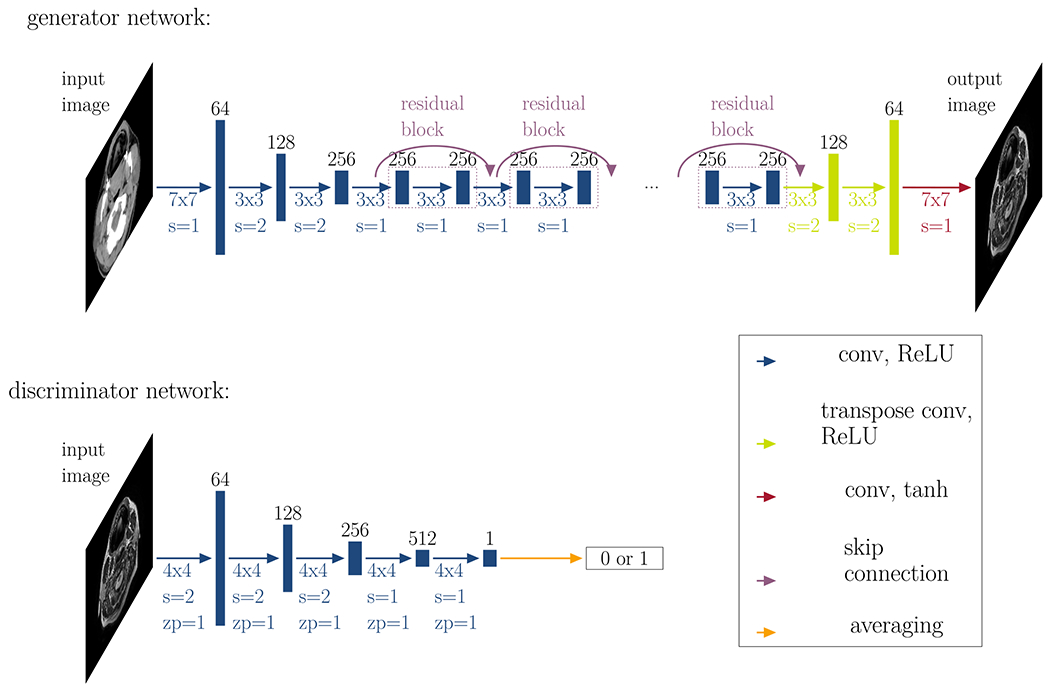
Generator and discriminator networks: This figure illustrates the generator network (top row) and the discriminator network (bottom row). The generator consists of three convolutional layers (conv) with a rectified linear activation function (ReLU), followed by nine residual blocks, two transpose convolutional layers, and a final convolutional layer with a tanh activation function. The discriminator consists of five convolutional layers and classifies images into two categories: real or fake. The black numbers on top of the layers represent the number of feature channels. Below each array, the colored numbers denote the convolutional kernel size (#x#), the size of the stride s and the size of potential zero-padding zp.

2.C.2. Training parameters

We employed the recommended training settings, as described in the original publication³² (Adam optimizer³⁸ with batch size 1, initial learning rate 2 × 10⁻⁴ fixed for 100 epochs and linearly decaying to zero over another 100 epochs, where in each epoch, the algorithm iterates over all training images.). For the respective contributions to the full objective function, which is composed of the weighted sum of the individual terms, we set the weights to λ_adversarial = 1 for the adversarial loss term, λ_cycle = 10 for the cycle-consistency terms, and λ_geo = 10 for the geometric consistency terms.

2.D. Data cleaning as input for segmentation network

Since not all synthetic MR images perfectly matched the input CT, we performed a data cleaning where we only selected slices that were suitable for the segmentation of the parotid glands. The selection was done based on the Dice overlap of the external outline of the head between the synthetic and real image where we discarded all images that had an overlap of less than 80%. Furthermore, we explored constraints on the external outline of the head and decided to perform a refinement 2D registration to map synthetic MR images to the original CT. We performed the registration using the Elastix toolkit³⁹ (rigid registration followed by deformable registration, CPP grid spacing: 8 mm, similarity measure: mutual information, optimizer: gradient descent). As the synthetic MR images were already generated in the same geometrical space as the CT, the segmentation of the CT formed the gold standard MR segmentation for the segmentation network.

2.E. Segmentation network

After data cleaning, we fed all remaining 2D synthetic MR images (approximately 1500) into a 2D U-Net as training data (step (2) of the workflow in Fig. 2). The U-net was trained to generate contours for the input MR images. Figure 5 illustrates the network’s architecture (5 resolution levels, starting at 64 features and ending at 1024 features at the lowest resolution in the bottleneck).

Fig 5.

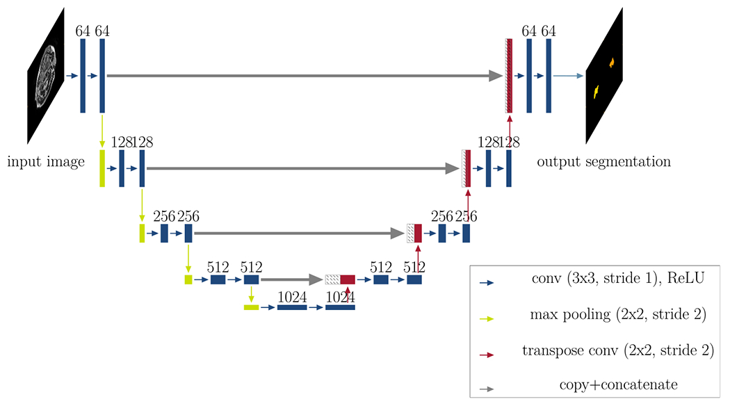
Network architecture: This figure illustrates the architecture of the segmentation network (2D U-Net with five resolution levels, starting at 64 features and ending at 1024 features at the lowest resolution in the bottleneck). Each rectangle corresponds to a feature map. The feature channels are denoted at the top of the rectangles. Striped boxes represent copied feature maps. The colored arrows denote the different operations as indicated in the legend. The output for all three approaches is a 2D segmentation map.

We split the data into 80% training and 20% validation to choose suitable hyperparameters. The inference was performed on the 27 real MR images, which comprised the testing data. We trained the segmentation network for 100 epochs with an initial learning rate of 5 × 10⁻⁵ We used the Adam optimizer³⁸ and a Dice similarity loss function. We gradually reduced the learning rate by monitoring the validation loss, down to a minimum of 10⁻⁷ and employed early stopping when the validation loss did not decrease by more than 1% after a patience of 10 epochs.

2.F. Computation time

The run times were determined for program execution on a single Tesla V100 with 16 GB VRAM. Inference times are stated per patient, where we calculated the average over all 27 patients, as well as the standard deviation.

2.G. Geometric evaluation

We evaluated the performance of the segmentation network by calculating the Dice similarity coefficient (DSC), Hausdorff distance (HD), and mean surface distance (MSD) between manual and auto-generated contours. We compared the determined accuracy to training the segmentation network with the CT data (CT only) as a benchmark. It is a known problem that the evaluation of auto-segmentation suffers from the lack of the ground truth. Interobserver variability can provide an estimate of the upper bound on the desired auto-segmentation accuracy. We compared our results to the interobserver variability which we had determined in a previous study.⁴⁰ That interobserver study was performed on a subset of the patients from this current study. In the referenced study, three observers including the one in our current study contoured the parotid glands. To determine the interobserver variability between two observers we first calculated the DSC, HD, and MSD between the respective observers’ contours for each patient and defined the variability as the average and SD over all patients. The overall interobserver variability was then calculated as the average of the three individual interobserver variabilities, with the SD being the root mean square of the three individual SDs.

3. RESULTS

3.A. Synthetic MR generation

Figure 6 illustrates selected (green box) and rejected (red box) example cases of synthetic MR images together with their corresponding source CT images. In most rejected cases, the synthetic MR images appeared as if they could be real MR images, however, they did not reflect the anatomy visible in the source CT images.

Fig 6.

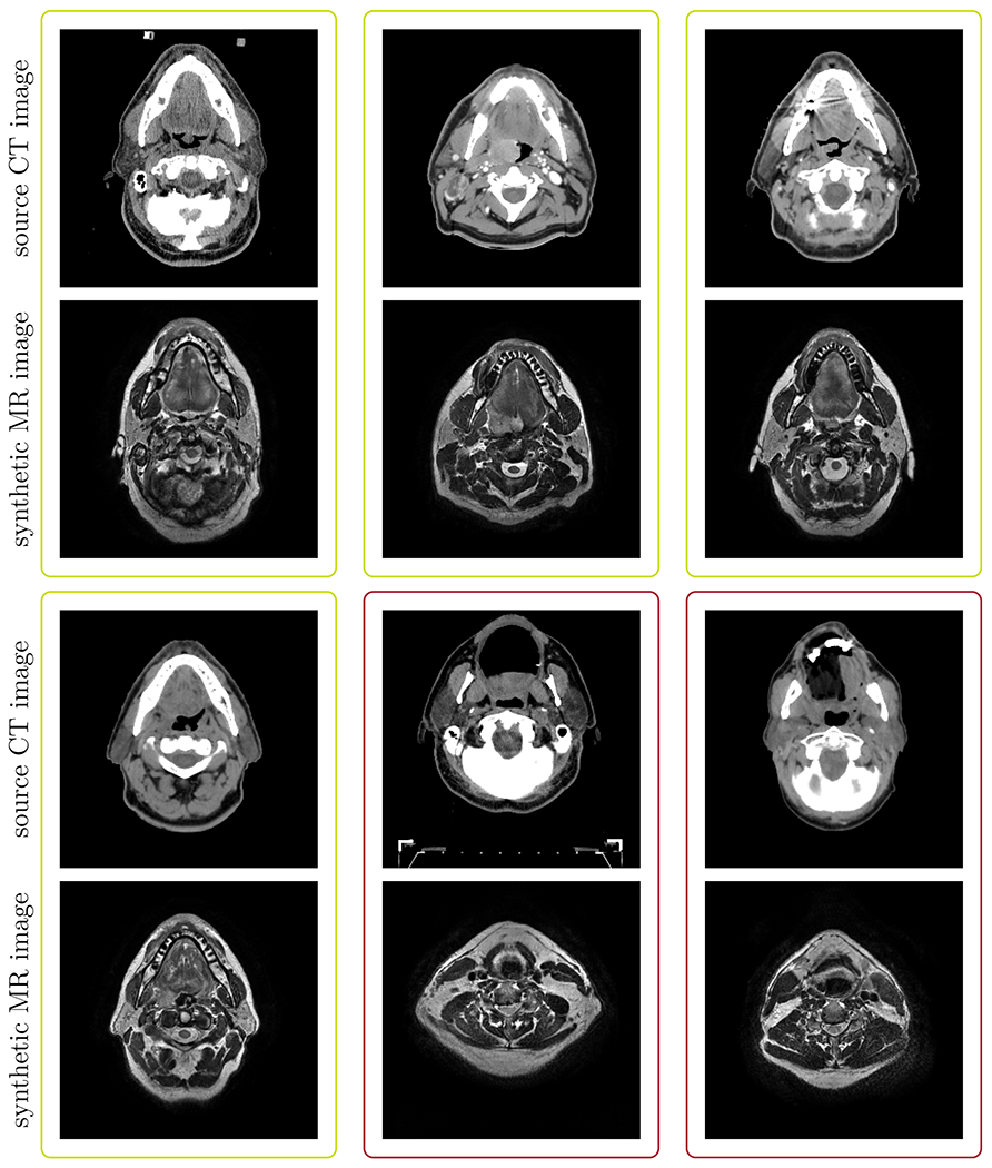
Typical examples of synthetic MRs and their corresponding source CTs: The green boxes highlight example cases that were selected for further learning. The red boxes highlight cases where the CycleGAN failed to produce anatomically corresponding MR images for the respective CT images and hence were rejected for further analysis.

3.B. Computation time

Training of the CycleGAN took approximately 72 h. The training of the 2D U-Net took approximately 150 min, whereas inference was done within 0.86±0.02s per patient.

3.C. Qualitative segmentation results

Figure 7 illustrates four typical example cases for autogenerated contours using the cross-modality approach, compared to the manual contours. We selected an axial, sagittal, and coronal view for each of the patients. The auto-generated contours followed the manual ones closely.

Fig 7.

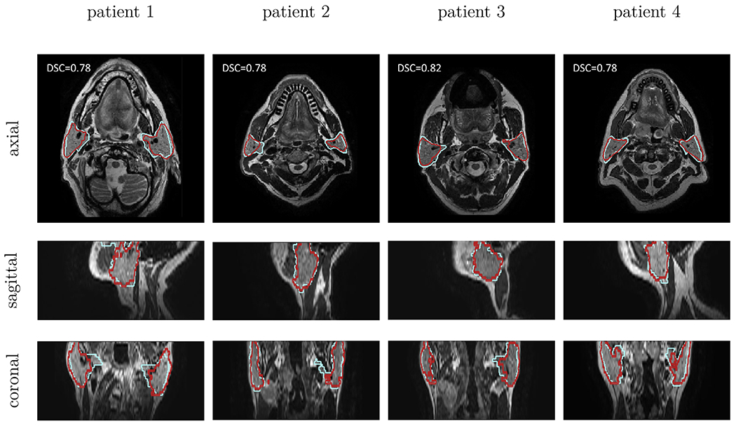
Qualitative results for cross-modality method: In each column a typical example case of the cross-modality learning approach (in red) is shown. The manual contours are shown in blue. The rows correspond to an axial, sagittal, and coronal cross-section, respectively. Each example originates from a different patient image.

3.D. Geometric evaluation

Figure 8 illustrates boxplots, comparing our developed method, cross-modality learning, to the CT-trained network. Table II lists mean and standard deviations for the DSC, HD, and MSD for all methods. The cross-modality learning accuracy (DSC: 0.77±0.07, HD: 18.32±10.12mm, MSD: 2.51±1.47mm) stayed below, but was close to the interobserver variability (0.84±0.04, 10.76±4.35mm, 1.40±0.45mm), as well as the CT-trained (DSC: 0.82±0.09, HD: 13.01 ±5.61mm, MSD: 1.81±0.99mm) network.

Fig 8.

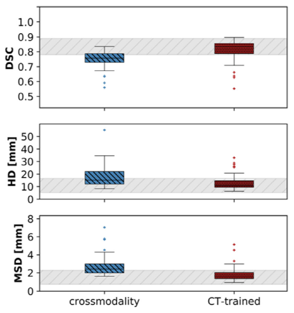
Boxplots of the Dice similarity coefficient, the Hausdorff distance and the mean surface distance (from top to bottom), averaged for both parotid glands. The introduced method (in red) is compared to the CT-trained network (in green). The gray bar represents the interobserver variability.⁴⁰

Table II.

Evaluation of the geometric accuracy of auto-segmenting the left and right parotid gland of the cross-modality learning approach (highlighted in bold). As a benchmark, we also include the geometric accuracy of the CT-trained network.

ROI	Method	$\stackrel{─}{DSC}$	$\stackrel{─}{HD}$ (mm)	$\stackrel{─}{MSD}$ (mm)
Right	Cross-modality learning	0.76 ± 0.06	18.32 ± 10.12	2.66 ± 1.26
Parotid	CT only	0.81 ± 0.07	13.01 ± 5.61	1.87 ± 0.84
	Interobserver variability	0.84 ± 0.04	10.76 ± 4.35	1.40 ± 0.45
Left	Cross-modality learning	0.77 ± 0.04	17.75 ± 7.49	2.36 ± 0.75
Parotid	CT only	0.82 ± 0.05	12.98 ± 5.15	1.74 ± 0.53
	Interobserver variability	0.83 ± 0.04	10.94 ± 3.75	1.59 ± 0.63

4. DISCUSSION

In this study, we employed a new technique, cross-modality learning, to transfer knowledge gained from one application (annotated CT images) to a new application (nonannotated MR images). This technique tackles the general problem of data scarcity in medical imaging. To the best of our knowledge, we were the first to generate synthetic MR images from annotated CT images to train an MR segmentation network. We found that it was possible to obtain decent quality annotations of MR images from annotated CT data.

We anticipate that cross-modality learning could be used to generally adapt a trained network of one imaging modality to another imaging modality. Auto-segmentation methods are usually trained on a very particular subset of imaging data. These might work well when the target images are similar to the ones that have been used in the development phase. However, in clinical routine, there are frequent changes, especially in MR image settings. While in a conventional approach this could mean that a new database with annotations of the new images would need to be created, the cross-modality learning would be able to reuse the already existing annotations on existing data and transfer it to the new data.

In this study we investigated the extreme case where no annotated MR data are available. In future work, one could combine real and synthetic MR data, for example by using the synthetic MR images as augmentation data, or by training the network with the synthetic data as initialization and fine-tune using the real MR data.

4.A. Synthetic MR generation

The CycleGAN was generally able to generate synthetic MR image from the input CT images. In the cases where it failed, the synthetic MR image often still looked like a real MR image, albeit not corresponding to the anatomy of the source CT image. Depending on the application, such images still could be useful. However, for our purpose, where we propagate the contours, one requires a satisfactory agreement between the represented anatomies. The failed generation could stem from the fact that we only had a small number of real MR images from which the CycleGAN could perform a style transfer. As the CycleGAN learns to map features from the source data (here: CT) to the target data (here: MR), it might focus on irrelevant features, such as smaller heads in the target data. Failure to generate an MR that corresponded well to the input CT especially happened at the superior and inferior boundary slices. Due to the limited field of view of the training MR images in that direction, there were not a lot of samples available for the CycleGAN to learn.

We furthermore detected a systematically narrower external outline of the head for the synthetic MR images compared to the source CT. In theory, no penalty in the CycleGAN prevents it from learning this narrowing function, as it could learn to generate more “narrow” MR images in the forward generator and go back to “broader” CT images in the backwards generator. This issue could be related to the skin outline being visible in the CT images but not in the MR images. While we tried to enforce a better overlay between these outlines by incorporating a geometric consistency penalty in the loss function, we were not able to entirely remove this issue. Wolterink et al.³³ did not report on any similar issues. However, they trained the CycleGAN using CT and corresponding MR images stemming from the same patients, whereas our study was aiming at datasets where there were no matched data available and the CT and MR images therefore originated from different patients, subject to a large variability within the dataset itself. A recent study has reported similar findings and introduced an additional shape-consistency loss to mitigate this problem.⁴¹

Recent research has shown that GANs are generally challenging to train and face problems with nonconvergence, mode collapse (producing limited varieties of samples) and diminishing gradients of the generator when the discriminator becomes too powerful.⁴² As they have been shown to be highly susceptible to hyperparameter selections,⁴² we expect that one could improve the synthetic MR generation further by tuning more hyperparameters. However, this would require more training data than what was available for this proof-of-concept study. Once more data become available, one could further optimize these parameters in future studies. In this study, we performed a 2D registration between the CT and the corresponding synthetic MR image to mitigate these detected “narrowing” transformations.

4.B. Geometric evaluation

The accuracy of the cross-modality method stayed below the interobserver variability, as well as the CT-trained network. We believe that there are several reasons for the crossmodality method to be inferior in segmentation quality compared to networks trained on real data and we believe that the accuracy of the network can be further improved if these issues are addressed adequately. The quality of the ground truth contours for the CT images was not as high as for the MR images. Three typical examples demonstrating the inferior quality of the CT contours are illustrated in Fig. 9.

Fig 9.

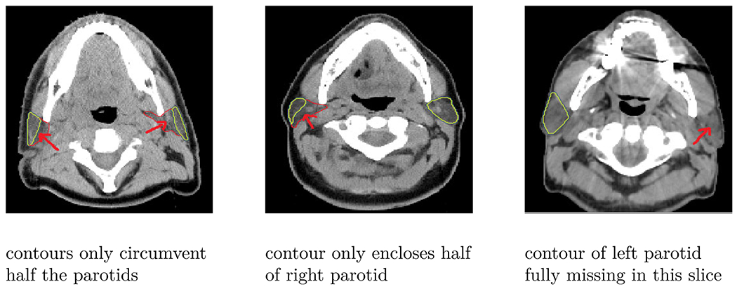
Quality of CT contours: This figure illustrates three typical example of poor quality CT contours, where the contours do not enclose the full parotids (left and right parotid in the first column, right parotid in the second column) or are fully missing (left parotid in the last column).

This was also evident from the accuracy of the CT-trained network. The MR images in this study were contoured by the observers specifically for the purpose of creating accurate contours, hence leading to a generally larger agreement. The CT data, on the other hand, were contoured in clinics for RT and not for a contouring study. The CT contours hence represent a typical clinical dataset. The MR contours used to evaluate the cross-modality method were done by a single observer, whereas the CT contours used as a reference for the CT-only training were done by multiple observers, introducing further uncertainty. We expect that the true agreement between observers in the CT dataset would be lower than what the interobserver variability from the MR data suggests. However, it was not possible to obtain this value for our study.

The cross-modality method was trained using the suboptimal contours of the CT dataset but was evaluated on the accurate contours of the MR dataset. The CT-only method, on the other hand, was compared to the suboptimal contours of the CT dataset. These reasons led to a worse performance for the cross-modality method per definition, when compared to the interobserver variability and the CT-only method. We believe that the cross-modality approach best represents the true performance, as in a commercial setting, the end user (e.g., clinician 1) will use a product that was trained on data from other clinicians (clinicians 2-N) and the end user will always compare the performance of the product to what he or she would have normally contoured. The CT-only method was only added as an optimal reference. The fact that the cross-modality method scored only marginally worse (the CT-only compared to cross-modality difference was included in the confidence intervals of 1 SD) is very encouraging.

We found two challenges in the synthetic MR generation. First, the synthetic MR images did not always represent the corresponding anatomy of the CT images and second, a registration between source CT and synthetic MR images was necessary. These challenges may have introduced a further inaccuracy in the segmentation network, hence resulting in a lower segmentation quality of the cross-modality learning method compared to training the network with the CT images.

In comparison to a transfer learning approach, we could directly incorporate the varieties found in a larger patient database to the small subset of MR images. Unlike in typical transfer learning applications, we did not merely want to transfer the ability to detect edges and simple shapes. Instead, we aimed to transfer the gained knowledge about the variety of shapes and locations of the parotid glands from the network trained on CT images. Additional experiments (not shown in this paper) have shown that it is challenging to determine where the desired information is stored in the networks and hence it is not straightforward to transfer that information to a new application. Furthermore, unlike the transfer learning approach, no additional manual segmentation was necessary with the cross-modality learning method.

4.C. Limitations of this study

A limitation of the introduced cross-modality learning was that 2D slices were predicted instead of directly generating 3D volumes. This led to inconsistencies between some slices and only allowed for a 2D segmentation network. Employing a fully 3D approach may reduce the number of falsely predicted synthetic MR images. However, current state of the art GPUs, including ours, are typically not able to train such a 3D CycleGAN due to insufficient memory.

In this proof-of-principle study, 2D image registration between the CT and synthetic MR slices was necessary. We are confident that in future work, when larger CT and MR databases become available, this need will be removed. Such databases would enable the CycleGAN to capture the important features in both imaging modalities and lead to better-quality synthetic MR images.

5. CONCLUSION

We employed cross-modality learning, to transform annotated CT images into synthetic annotated MR images. These synthetic MR images were of sufficient quality to train a network for automated contouring. This technique of crossmodality learning can be of great value for segmentation problems where annotated training data are sparse. We anticipate using this method with any MR training dataset to generate synthetic MR images of the same type via image style transfer from CT images. Furthermore, as this technique allows for fast adaptation of annotated datasets from one imaging modality to another, it could prove to be useful for translating between large varieties of MRI contrasts due to differences in imaging protocols within and between institutions.

REFERENCES

- 1.Daisne J-F, Blumhofer A. Atlas-based automatic segmentation of head and neck organs at risk and nodal target volumes: a clinical validation. Radiat Oncol. 2013;8:154. [DOI] [PMC free article] [PubMed] [Google Scholar]
- 2.Geets X, Daisne J-F, Arcangeli S, et al. Inter-observer variability in the delineation of pharyngo-laryngeal tumor, parotid glands and cervical spinal cord: comparison between CT-scan and MRI. Radiother Oncol. 2005;77:25–31. [DOI] [PubMed] [Google Scholar]
- 3.Vinod SK, Jameson MG, Min M, Holloway FC. Uncertainties in volume delineation in radiation oncology: a systematic review and recommendations for future studies. Radiother Oncol. 2016;121:169–179. [DOI] [PubMed] [Google Scholar]
- 4.Cardenas CE, Yang J, Anderson BM, Court LE, Brock KB. Advances in auto-segmentation. Sem Radiat Oncol. 2019;29:185–197. [DOI] [PubMed] [Google Scholar]
- 5.Ibragimov B, Xing L. Segmentation of organs-at-risks in head and neck CT images using convolutional neural networks. Med Phys. 2017;44:547–557. [DOI] [PMC free article] [PubMed] [Google Scholar]
- 6.Tong N, Gou S, Yang S, Ruan D, Sheng K. Fully automatic multi-organ segmentation for head and neck cancer radiotherapy using shape representation model constrained fully convolutional neural networks. Med Phys. 2018;45:4558–4567. [DOI] [PMC free article] [PubMed] [Google Scholar]
- 7.Močnik D, Ibragimov B, Xing F, et al. Segmentation of parotid glands from registered CT and MR images. Physica Med. 2018;52:33–41. [DOI] [PMC free article] [PubMed] [Google Scholar]
- 8.Chan JW, Kearney V, Ms SH, et al. A convolutional neural network algorithm for automatic segmentation of head and neck organs-at-risk using deep lifelong learning. Med Phys. 2019;9785:97850Y. [DOI] [PubMed] [Google Scholar]
- 9.van Rooij W, Dahele M, Brandao HR, Delaney AR, Slotman BJ, Verbakel WF. Deep learning-based delineation of head and neck organs-at-risk: geometric and dosimetric evaluation. Int J Radiat Oncol Biol Phys. 2019;104:677–684. [DOI] [PubMed] [Google Scholar]
- 10.Fontanarosa D, Van Der Meer S, Bamber J, Harris E, O’Shea T, Verhaegen F. Review of ultrasound image guidance in external beam radiotherapy: I. Treatment planning and inter-fraction motion management. Phys Med Biol. 2015;60:R77. [DOI] [PubMed] [Google Scholar]
- 11.Grosu AL, Piert M, Weber WA, et al. Positron emission tomography for radiation treatment planning. Strahlenther Onkol. 2005;181:483–499. [DOI] [PubMed] [Google Scholar]
- 12.Delouya G, Igidbashian L, Houle A, et al. 18F-FDG-PET imaging in radiotherapy tumor volume delineation in treatment of head and neck cancer. Radiother Oncol. 2011;101:362–368. [DOI] [PubMed] [Google Scholar]
- 13.Metcalfe P, Liney GP, Holloway L, et al. The potential for an enhanced role for MRI in radiation-therapy treatment planning. TechCancer Res Treat. 2013;12:429–446. [DOI] [PMC free article] [PubMed] [Google Scholar]
- 14.Dirix P, Haustermans K, Vandecaveye V. The value of magnetic resonance imaging for radiotherapy planning. Sem Radiat Oncol. 2014;24:151–159. [DOI] [PubMed] [Google Scholar]
- 15.Lagendijk JJ, Raaymakers BW, Van Den Berg CA, Moerland MA, Philippens ME, Van Vulpen M. MR guidance in radiotherapy. Phys Med Biol. 2014;59:R349–R369. [DOI] [PubMed] [Google Scholar]
- 16.Wong KH, Panek R, Bhide SA, Nutting CM, Harrington KJ, Newbold KL. The emerging potential of magnetic resonance imaging in personalizing radiotherapy for head and neck cancer: an oncologist’s perspective. Br J Radiol. 2017;90:20160768. [DOI] [PMC free article] [PubMed] [Google Scholar]
- 17.Raaymakers BW, Lagendijk JJW, Overweg J, et al. Integrating a 1.5 T MRI scanner with a 6 MV accelerator: proof of concept. Phys Med Biol. 2009;54:N229–N237. [DOI] [PubMed] [Google Scholar]
- 18.Fallone BG, Murray B, Rathee S, et al. First MR images obtained during megavoltage photon irradiation from a prototype integrated linac-MR system. Med Phys 2009;36:2084–2088. [DOI] [PubMed] [Google Scholar]
- 19.Mutic S, Dempsey JF. The ViewRay system: magnetic resonance-guided and controlled radiotherapy. Sem Radiat Oncol. 2014;24:196–199. [DOI] [PubMed] [Google Scholar]
- 20.Liney GP, Dong B, Begg J, et al. Technical note: experimental results from a prototype high-field inline MRI-linac. Med Phys. 2016;43: 5188–5194. [DOI] [PubMed] [Google Scholar]
- 21.Western C, Hristov D, Schlosser J. Ultrasound imaging in radiation therapy: from interfractional to intrafractional guidance. Cureus. 2015;7:1–19. [DOI] [PMC free article] [PubMed] [Google Scholar]
- 22.Camps SM, Fontanarosa D, de With PHN, Verhaegen F, Vanneste BGL. The use of ultrasound imaging in the external beam radiotherapy workflow of prostate cancer patients. BioMed Research International. 2018;2018:1–16. [DOI] [PMC free article] [PubMed] [Google Scholar]
- 23.Simard P, Victorri B, LeCun Y, Denker J. Tangent prop-a formalism for specifying selected invariances in an adaptive network. In: NIPS; 1992. [Google Scholar]
- 24.LeCun Y, Bengio Y, Hinton G. Deep learning. Nat Methods. 2015; 13:35. [DOI] [PubMed] [Google Scholar]
- 25.Cheplygina V Cats or CAT scans: transfer learning from natural or medical image source datasets?. Current Opinion Biomed Eng. 2018;9:21–27. [Google Scholar]
- 26.Schlegl T, Ofner J, Langs G. Unsupervised pre-training across imagedo-mains improves lung tissue classification. Medical Computer Vision: Algorithms for Big Data (MICCAI MCV). Berlin: Springer; 2014:82–93. [Google Scholar]
- 27.Bar Y, Diamant I, Wolf L, Lieberman S, Konen E, Greenspan H. Chest pathology detection using deep learning with non-medical training. In: Proceedings - International Symposium on Biomedical Imaging; 2015. [Google Scholar]
- 28.Goodfellow IJ, Pouget-Abadie J, Mirza M, et al. Generative adversarial networks 2014;1–9. [Google Scholar]
- 29.Isola P, Zhu JY, Zhou T, Efros AA. Image-to-image translation with conditional adversarial networks. In: Proceedings - 30th IEEE Conference on Computer Vision and Pattern Recognition, CVPR 2017; 2017. [Google Scholar]
- 30.Bowles C, Chen L, Guerrero R, et al. GAN augmentation: augmenting training data using generative adversarial networks; 2018. [Google Scholar]
- 31.Frid-Adar M, Diamant I, Klang E, Amitai M, Goldberger J, Greenspan H. GAN-based synthetic medical image augmentation for increased CNN performance in liver lesion classification. Neurocomputing. 2018;321:321–331. [Google Scholar]
- 32.Zhu JY, Park T, Isola P, Efros AA. Unpaired image-to-image translation using cycle-consistent adversarial networks. In: Proceedings of the IEEE International Conference on Computer Vision. Vol. 2017-Octob; 2242–2251; 2017. [Google Scholar]
- 33.Wolterink JM, Dinkla AM, Savenije MH, Seevinck PR, van den Berg CA, Išgum I. Deep MR to CT synthesis using unpaired data. In: Lecture Notes in Computer Science (including subseries Lecture Notes in Artificial Intelligence and Lecture Notes in Bioinformatics). Vol. 10557. Cham: Springer; 2017:14–23. [Google Scholar]
- 34.Grossberg AJ, Mohamed ASR, Elhalawani H, et al. Data from head and neck cancer CT atlas. The Cancer Imaging Archive. 2017. [Google Scholar]
- 35.Raudaschl PF, Zaffino P, Sharp GC, et al. Evaluation of segmentation methods on head and neck CT: auto-segmentation challenge 2015. Med Phys. 2017;44:2020–2036. [DOI] [PubMed] [Google Scholar]
- 36.Hoang JK, Glastonbury CM, Chen LF, Salvatore JK, Eastwood JD. CT mucosal window settings: a novel approach to evaluating early T-stage head and neck carcinoma. Am J Roentgenol. 2010;195:1002–1006. [DOI] [PubMed] [Google Scholar]
- 37.Paszke A, Chanan G, Lin Z, et al. Automatic differentiation in PyTorch. In: NIPS; 2017. [Google Scholar]
- 38.Kingma DP, Ba JL. Adam: a method for stochastic gradient descent. arXiv preprint; 2014. [Google Scholar]
- 39.Klein S, Staring M, Murphy K, Viergever MA, Pluim JP. Elastix: a toolbox for intensity-based medical image registration. IEEE Trans Med Imaging. 2010;29:196–205. [DOI] [PubMed] [Google Scholar]
- 40.Kieselmann JP, Kamerling CP, Burgos N, et al. Geometric and dosimetric evaluations of atlas-based segmentation methods of MR images in the head and neck region. Phys Med Biol. 2018;63:145007. [DOI] [PMC free article] [PubMed] [Google Scholar]
- 41.Zhang Z, Yang L, Zheng Y. Translating and segmenting multimodal medical volumes with cycle- and shape-consistency generative adversarial network. n: Proceedings of the IEEE Computer Society Conference on Computer Vision and Pattern Recognition; 2018. [Google Scholar]
- 42.Goodfellow IJ. NIPS 2016 tutorial: generative adversarial networks; 2016. [Google Scholar]