Probabilistic Model for Control of an Epidemic by Isolation and Quarantine

Abstract

Assuming a homogeneous population, we apply the mass action law for rate of new infections and a second-order gamma distribution for removal probability to model spread of an epidemic. In numerical examinations of higher-order gamma distributions for removal probability, we discover an unexpected pattern in maximum fraction of population infected. We develop from first principles of probability an eighth-order system of ordinary differential equations to model effects of isolation and quarantine. We derive analytical expressions for reproduction numbers modeling isolation and quarantine when applied separately and together and verify them numerically. We quantify strength and speed required of these interventions to contain epidemics of varying severity and examine how their effectiveness depends on when they begin. We find that effectiveness is highly sensitive to small changes of intervention strength in a critical region. Finally, adding two more differential equations to capture natural population dynamics, we calculate endemic disease equilibria when affected by isolation and examine dynamics of coming to an equilibrium state.

Introduction

Mathematical epidemiology has a long history. In 1760, Daniel Bernoulli analyzed inoculation against smallpox, where he developed what is usually described as the first model in the subject (Bernoulli 1766; Blower 2004; Heesterbeck and Roberts 2015).

On developments directly relevant to the matter at hand, in 1906 Hamer proposed a mass action law, in which rate of new infections in a disease outbreak is proportional to the product of the number of susceptible individuals and the number of infected individuals. This model has been widely used since that time (Hamer 1906; Brauer 2017).

Kermack and McKendrick (1927) introduced compartments to model spread of infectious diseases. A special case of their general model is referred to as the SIR model, with compartments S (susceptible but well), I (infected and able to transmit the disease) and R (removed by immunity, recovery, death or quarantine). In this model, people who recover are permanently immune. The SIR model incorporates the mass action law and has become the starting point for a wide variety of compartmental models to the present day. The SIR model is deterministic, meaning it incorporates no element of chance. We will discuss the SIR model more, later in this article.

Beginning in 1928 and continuing through the 1930s and 1940s, L. J. Reed and W. H. Frost lectured at what is now the Johns Hopkins Bloomberg School of Public Health and developed the stochastic Reed–Frost model, which has been widely used and from which many extensions have been formulated (Lessler and Cummings 2016; Brauer 2017). Their work was published by their students (Abbey 1952; De Maia 1952). Stochastic models include the element of chance. We will discuss the Reed-Frost model more, later in this article.

Isolation is removal of an infected person from public interaction. Quarantine is removal of a segment of the population, regardless of health condition, usually by government order. A deterministic study by Hethcote et al. (2002) modeled compartments SIQR and SIQS. In the latter, people who recover are not immune but rather return to susceptibility. The compartment labeled Q was for isolation, in that transitions to Q were from I only. The analysis found conditions under which disease can be endemic, i.e., have a permanent presence. In some cases, the presence was a stable, constant equilibrium. In others, it was eventually periodic.

Gumel et al. (2004) authored a study on strategies for controlling SARS (severe acute respiratory syndrome) outbreaks. They used a deterministic SEQIJR model, where Q and J were for quarantine and isolation and E labeled a compartment for the exposed but asymptomatic. In the Hethcote et al. study above, the Gumel et al. study and most compartment-based studies, transitions between compartments are modeled as first-order, linear, single-parameter rates except for rate of new infections, which is modeled by various versions of the mass action law. In the Gumel et al. study, transitions to the quarantine compartment were from the exposed compartment only, which implies they were based on contact tracing. The study compared model predictions to actual outcomes in a number of geographic areas and found good agreement. It also showed the benefit of fast response in both isolation and quarantine together.

The literature has many articles analyzing isolation and quarantine that are based on compartmental models. Many are deterministic (e.g., Castillo-Chavez et al. 2003; Sahu and Dhar 2015; Denes and Gumel 2019) and some are stochastic by virtue of adding Wiener processes (e.g., Li et al. 2018). The latter require multiple solutions of the equations to produce multiple realizations of an epidemic in order to yield reliable “expected value” results (Monte Carlo simulation).

All the isolation and quarantine models discussed above assume a homogeneous population. Other studies using the same assumption but not employing compartmental models include Day et al. (2006), which used a discrete time branching process, and Fraser et al. (2004), which utilized partial differential equations of the transport type.

Even if populations were homogeneous, compartmental models are inadequate for the very early dynamics of epidemics (Diekmann et al. 2013; Brauer 2017). Important fluctuations in initial spread are represented much better by network branching processes.

Spatial, age and demographic heterogeneity are real-life conditions that require additional model sophistication. The professional standard is set by immense computer programs that account for actions of millions of people individually: their age, demographic status and location, with real data on such matters as airline schedules from city to city. The programs are stochastic but so large that only a few realizations can feasibly be produced, even on supercomputers. Halloran et al. (2008), Ferguson et al. (2006), German et al. (2006) and Lewis et al. (2007) are examples.

In today’s world, the sophisticated technologies described above are essential. But simple models have a place. With minimal time and effort, simple models can enable preliminary assessment of a wide range of strategic policy options and point the way to more in-depth studies. They can be useful introductory educational tools for those entering the epidemiology profession. Furthermore, even for basic subjects such as isolation and quarantine, a simple model can quantify, with a broad brush, effort required to contain an epidemic and clearly demonstrate how deleterious delay and noncompliance can be. Finally, it can identify endemic equilibria, conditions portending a long-term struggle against the disease.

This article develops and employs such a model.

Section 2 develops the model from first principles of probability as it applies to unmitigated spread of an epidemic. Section 3 compares that model to the SIR equations and finds an interesting ratio in maximum fraction of population infected, which Sect. 4 explores further. Applying first principles of probability, Sect. 5 extends the model to include effects of isolation and quarantine. Section 6 employs the model to (a) determine requirements on isolation and quarantine to contain an epidemic, (b) quantify mitigation effectiveness as it depends on when intervention begins and (c) measure consequences of efforts falling short. It finds that intervention effectiveness is highly sensitive to small changes of effort in a critical region. Section 7 extends the model once more to examine endemic disease equilibria when affected by isolation. Finally Sect. 8 reviews main points of the article and summarizes advantages and disadvantages we perceive in this model with respect to others in the literature.

Developing the Basic Probabilistic Model

Let

• ${\widehat{s}}_j(t)=$ conditional probability that individual $j$ in a population of $N$ people is susceptible to the disease but has not contracted it after time $t$ since its outbreak, given the sequence of contacts and times $t_k$, $k=1,\dots ,{\widehat{n}}_j(t)$.

• ${\widehat{i}}_j(t_k)=$ probability that the person with whom individual $j$ interacted in his or her $k$ th interaction since disease outbreak was infected at time of interaction.

• $c=$ probability that the disease is transmitted in a single interaction between a susceptible-but-well person and an infected one.

• ${\widehat{n}}_j(t)=$ number of interactions individual $j$ has had with other people by time $t$.

Then, ${\widehat{s}}_j(t)$ is given by the product of the probabilities of the individual not being infected on each of his or her ${\widehat{n}}_j(t)$ interactions:

$${\widehat{s}}_j(t)=\prod _{k=1}^{{\widehat{n}}_j(t)}(1-c{\widehat{i}}_j(t_k)).$$ 1

We are assuming for simplicity that no one is initially immune.

Equation (1) is a form of the Reed-Frost model. The variables ${\widehat{n}}_j(t)$, ${\widehat{s}}_j(t)$ and ${\widehat{i}}_j(t)$ are stochastic processes. The number ${\widehat{n}}_j(t)$ takes on only integer values, increasing by one at randomly occurring interactions. Any realization of ${\widehat{s}}_j(t)$ is constant between interactions, where it takes discontinuous steps down. From this, we form a deterministic, differentiable function by taking expected values.

Averaging over all possible interactions, the individuals involved and when,

$$\begin{array}{c}{s}_j(t)=E\left\{{\widehat{s}}_j(t)\right\}\\ i_j(t)=E\left\{{\widehat{i}}_j(t)\right\}\\ \end{array}$$

We assume that interaction times follow a homogeneous Poisson process with growth rate $a$, assumed constant. Let $X={\widehat{n}}_j(t+\mathrm{\Delta }t)-{\widehat{n}}_j(t)$. Then $X$ is Poisson distributed with mean $a\mathrm{\Delta }t$. We also assume that $i_j(t)$ changes little in the small $\mathrm{\Delta }t$ interval. Then we can approximate

$$\begin{array}{cc}& s_j(t+\mathrm{\Delta }t)=E\left\{\prod _{k=1}^{{\widehat{n}}_j(t+\mathrm{\Delta }t)}(1-c{\widehat{i}}_j(t_k))\right\}\cong E\left\{\prod _{k=1}^{{\widehat{n}}_j(t)}(1-c{\widehat{i}}_j(t_k))\right\}{E}_X\left\{{(1-c{i}_j(t))}^X\right\}\hfill \\ \hfill & s_j(t+\mathrm{\Delta }t)=s_j(t)E_X\left\{{(1-c{i}_j(t))}^X\right\}.\hfill \\ \hfill \end{array}$$ 2

Now

$$E_X\left\{{(1-c{i}_j(t))}^X\right\}=exp(-a\mathrm{\Delta }t)\sum _{k=0}^{\infty }\frac{{(1-c{i}_j(t))}^k{(a\mathrm{\Delta }t)}^k}{k!}=exp(-c{i}_j(t)a\mathrm{\Delta }t).$$

So

$$s_j(t+\mathrm{\Delta }t)=s_j(t)exp(-c{i}_j(t)a\mathrm{\Delta }t).$$

Assuming homogeneity of the population, this becomes

$$s(t+\mathrm{\Delta }t)=s(t)exp(-ci(t)a\mathrm{\Delta }t).$$ 3

Then

$$\frac{s(t+\mathrm{\Delta }t)-s(t)}{\mathrm{\Delta }t}=s(t)\frac{exp(-ci(t)a\mathrm{\Delta }t)-1}{\mathrm{\Delta }t}.$$

Taking the limit as $\mathrm{\Delta }t\to 0$,

$$\frac{\mathrm{d}s}{\mathrm{d}t}=-acsi.$$ 4

This is the aforementioned mass action law. We have developed a well-known deterministic model from a well-known stochastic one. The fundamentals of this relationship are discussed in basic texts (e.g., Diekmann et al. 2013). We have included a bare sketch of the derivation to show the probabilistic underpinnings of our model. For a detailed rigorous proof, see Kurtz (1981). The product $\mathit{ac}$ is often denoted $\beta$, and we will follow that custom henceforth.

Next, we must derive an equation for $i(t)$. Let $r(t)$ be the probability a given person has been infected at some time in the epidemic but has been removed via recovery or death by time $t$. We assume that a person who recovers is permanently immune. To compute $r(t)$, we begin with the probability distribution

$$\mathrm{Prob}\{\mathrm{removal}\mathrm{by}\mathrm{time}t\mathrm{given}\mathrm{infection}\mathrm{at}\mathrm{time}\tau \}=r(t\left|\tau )=1-(1+{\gamma }_R(t-\tau ))exp(-{\gamma }_R(t-\tau ))\right)$$ 5

which has probability density ${\gamma }_R^2(t-\tau )exp(-{\gamma }_R(t-\tau ))$. This says an infected person is more likely to be removed at a time $1/{\gamma }_R$ after onset of infection than at any other time. Equation (5) is the second member of the Erlang family of distributions, which is the subset of the gamma family having integer order.

Let $p(t)$ be the probability a given person was infected at some time prior to $t$ in the epidemic. Then

$$s=1-p.$$ 6

The state equation for $p$ is

$$\frac{\mathrm{d}p}{\mathrm{d}t}=\beta si.$$ 7

Also,

$$i=p-r$$ 8

if we assume that deaths due to the epidemic are not an appreciable fraction of the population. It is convenient to say here only that a nonconstant circulating population is a complication and to defer further explanation of the need for this assumption to Sect. 5.

From Eq. (5) and definition of $p$:

$$r(t)={\int }_0^t\dot{p}(\tau )(1-(1+{\gamma }_R(t-\tau ))exp(-{\gamma }_R(t-\tau )))\mathrm{d}\tau .$$ 9

Integrating by parts:

$$r(t)={\int }_0^{t}p(\tau ){\gamma }_R^2(t-\tau ))exp(-{\gamma }_R(t-\tau )))\mathrm{d}\tau .$$ 10

Numerical values for $r(t)$ as given by Eq. (10) can be computed most readily by the following general process. Anticipating needs later in this paper, we consider an equation of the form

$${\alpha }_0(t)={\int }_0^t\left(\sum _{m=0}^n{k}_m{(t-\tau )}^m\right)exp(-\lambda (t-\tau ))\xi (\tau )\mathrm{d}\tau .$$ 11

Differentiating:

$$\frac{\mathrm{d}{\alpha }_0}{\mathrm{d}t}=k_0\xi (t)+{\int }_0^t\left(\sum _{m=1}^{n}m{k}_m{(t-\tau )}^{m-1}\right)exp(-\lambda (t-\tau ))\xi (\tau )\mathrm{d}\tau -\lambda {\alpha }_0.$$ 12

Denote the second term on the right-hand side of Eq. (12) as $\lambda {\alpha }_1$. Then, Eq. (12) becomes

$$\frac{\mathrm{d}{\alpha }_0}{\mathrm{d}t}=k_0\xi (t)+\lambda ({\alpha }_1-{\alpha }_0).$$ 13

Differentiating ${\alpha }_1$:

$$\frac{\mathrm{d}{\alpha }_1}{\mathrm{d}t}=\left(\frac{k_1}{\lambda }\right)\xi (t)+\frac{1}{\lambda }{\int }_0^t\left(\sum _{m=2}^{n}m(m-1)k_m{(t-\tau )}^{m-2}\right)exp(-\lambda (t-\tau ))\xi (\tau )\mathrm{d}\tau -\lambda {\alpha }_1.$$ 14

Denote the second term on the right-hand side of Eq. (14) as $\lambda {\alpha }_2$. Continuing in this way

$$\frac{\mathrm{d}{\alpha }_1}{\mathrm{d}t}=\left(\frac{k_1}{\lambda }\right)\xi (t)+\lambda ({\alpha }_2-{\alpha }_1)$$ 15

$$\frac{\mathrm{d}{\alpha }_m}{\mathrm{d}t}=\left(\frac{m!k_m}{{\lambda }^m}\right)\xi (t)+\lambda ({\alpha }_{m+1}-{\alpha }_m)(1<m<n)$$ 16

$$\frac{\mathrm{d}{\alpha }_n}{\mathrm{d}t}=\left(\frac{n!k_n}{{\lambda }^n}\right)\xi (t)-\lambda {\alpha }_n.$$ 17

Numerically integrating the simultaneous ordinary differential Eqs. (13), (15), (16) and (17) gives numerical values to ${\alpha }_0(t)$ as given by Eq. (11).

Translating Eq. (10) into the general form in Eq. (11) results in the following equations for $r(t)$:

$$\frac{\mathrm{d}r}{\mathrm{d}t}={\gamma }_R(r_1-r)$$ 18

$$\frac{\mathrm{d}{r}_1}{\mathrm{d}t}={\gamma }_R(p-r_1).$$ 19

Equations (6), (7), (8), (18) and (19) constitute our basic model, applying to spread of an unmitigated epidemic. For simplicity and consistency, we will refer to it as the basic probabilistic model, although at this point, as we will see in the next section, it differs from the SIR model only in the equation for removal probability. The name probabilistic model will be more fitting when, using first principles of probability, we extend it to include isolation and quarantine in Sect. 5 and natural population dynamics in Sect. 7.

Comparison with the SIR Model

The SIR equations can be written

$$\frac{\mathrm{d}s}{\mathrm{d}t}=-\beta si$$ 20

$$\frac{\mathrm{d}i}{\mathrm{d}t}=\beta si-\gamma i$$ 21

$$\frac{\mathrm{d}r}{\mathrm{d}t}=\gamma i.$$ 22

(See, e.g., Hethcote 2000.)

It is not difficult to show that the SIR model assumes

$$\mathrm{Prob}\{\mathrm{removal}\mathrm{by}\mathrm{time}t\mathrm{given}\mathrm{infection}\mathrm{at}\mathrm{time}\tau \}=1-exp(-\gamma (t-\tau ))$$ 23

and for brevity we omit the proof. Equation (23) is the first member in the Erlang family of probability distributions. The probability density for the distribution in Eq. (23) is $\gamma exp(-\gamma (t-\tau ))$, which says that an infected person is more likely to recover immediately after infection than at any later time. This is unrealistic, as discussed, e.g., in Diekmann et al. (2013), so we prefer to use the probability distribution in Eq. (5).

The SIR equations are attractive for their simplicity and utility. Two important measures of epidemic severity are (a) $s_{\infty }$, probability that a person chosen at random from the population is susceptible but well at the end of the epidemic and (b) $i_{\mathrm{MAX}}$, maximum probability of that person being infected (largest fraction of the population infected at any one time) during the epidemic. Derivations of the SIR model’s well-known equations for these measures are included here for convenience.

Setting $\mathrm{d}i/\mathrm{d}t=0$ in Eq. (21), we find that $s=\gamma /\beta$ is the fraction of people susceptible but well when the number of people infected in the epidemic reaches its peak. Using Eqs. (20) and (21), we find that

$$\frac{\mathrm{d}i}{\mathrm{d}s}=\frac{\mathrm{d}i}{\mathrm{d}t}·\frac{\mathrm{d}t}{\mathrm{d}s}=\frac{\mathrm{d}i/\mathrm{d}t}{\mathrm{d}s/\mathrm{d}t}=-1+\left(\gamma /\beta \right)(1/s).$$

Integrating:

$$i=1-s+\left(\gamma /\beta \right)ln\left(s\right).$$ 24

Setting $s=\gamma /\beta$ yields

$$i_{\mathrm{MAX}}=1-(\gamma /\beta )+(\gamma /\beta )ln(\gamma /\beta ).$$ 25

Setting $i=0$ in Eq. (24), we have

$$s_{\infty }-(\gamma /\beta )ln(s_{\infty })=1.$$ 26

Equation (26) applies beyond the SIR model, as we will discuss.

To compare the SIR and the basic probabilistic model quantitatively, we must find common ground, setting each model’s parameters so they represent the same severity of epidemic. Common ground is found in the basic reproduction number $R_0$. $R_0$ can be defined as the expected number of cases directly generated by one infected person in a population where all other individuals are susceptible to infection. Mathematically,

$$\begin{array}{cc}& R_0={\int }_0^{\infty }\mathrm{Prob}\{\mathrm{infected}\mathrm{person}\mathrm{is}\mathrm{in}\mathrm{circulation}\mathrm{at}\mathrm{time}t\}·\mathrm{average}\mathrm{contact}\mathrm{rate}\mathrm{at}\mathrm{time}\hfill \\ \hfill & t·\mathrm{Prob}\{\mathrm{transmitting}\mathrm{infection}\mathrm{on}\mathrm{one}\mathrm{interaction}\mathrm{at}\mathrm{time}t\}\mathrm{d}t\hfill \\ \hfill \end{array}$$ 27

For the SIR model, as is well-known and easy to prove:

$$R_0=\beta /\gamma .$$

For the basic probabilistic model:

• contact (interaction) rate at time $t=a$.

• probability of transmitting infection on one interaction at time $t=c$.

• probability that infected person is in circulation at time $t=1-r(t\left|0)=(1+{\gamma }_{R}t)exp(-{\gamma }_{R}t)\right)$

So for the basic probabilistic model,

$$R_0=ac{\int }_0^{\infty }(1+{\gamma }_{R}t)exp(-{\gamma }_{R}t)\mathrm{d}t=2ac/{\gamma }_R=2\beta /{\gamma }_R.$$ 28

Therefore, to compare the SIR and basic probabilistic models we set ${\gamma }_R=2\gamma$.

Figure 1 graphs $s_{\infty }$ and Fig. 2 graphs $i_{\mathit{MAX}}$ for the two models as a function of basic reproduction number. Numerical integration was accomplished with the Adams–Moulton algorithm.

Fig. 1.

Computing $s_{\infty }$ as a function of basic reproduction number $R_0$. The SIR model and basic probabilistic model give the same result

Fig. 2.

Comparing the basic probabilistic model to the SIR model in computation of $i_{\mathrm{MAX}}$ as a function of basic reproduction number $R_0$

There has been interest in the generality of the final size formula, which is Eq. (26) with $\beta /\gamma$ replaced by $R_0$. (Final size is defined as $1-s_{\infty }$.) For example, Ma and Earn (2006) demonstrate that the formula applies to three SIR variations. Figure 1 shows that the final size formula applies as well to the basic probabilistic model. In fact, Anderson and Watson (1980) proved that, for SIR-like models, removal probabilities given by gamma distributions of any order yield the same final size.

Figure 2 shows that $i_{\mathrm{MAX}}$ for the probabilistic model can be considerably larger than that for the SIR model. Interestingly, to the accuracy of our numerical integration, the ratio of $i_{\mathrm{MAX}}$ for the second-order removal distribution is 4/3 that for the SIR model as $R_0$ approaches one. This curious result will divert us temporarily to a mathematical sidebar in the next section. The ratio is not greatly different from 4/3 when $R_0$ is much larger; e.g., the ratio is 1.300 when $R_0$ is 2.75.

Mathematical Sidebar

We consider the SIR model with higher-order members of the Erlang family of probability distributions for the removal process. That is, we consider equation sets of the form

$$\begin{array}{cc}\hfill \frac{\mathrm{d}p}{\mathrm{d}t}& =\beta si,s=1-p,i=p-x_1\hfill \\ \hfill \frac{\mathrm{d}{x}_m}{\mathrm{d}t}& =n\gamma (x_{m+1}-x_m)1\le m<n\hfill \\ \hfill \frac{\mathrm{d}{x}_n}{\mathrm{d}t}& =n\gamma (p-x_n)\hfill \\ \hfill \end{array}$$ 29

which produce a SIR-like model with removal probability density

$$f(t-\tau )=\frac{1}{(n-1)!}{(n\gamma )}^n{(t-\tau )}^{n-1}exp(-n\gamma (t-\tau ))$$ 30

where $t-\tau$ is time since onset of infection and $1/\gamma$ the average time from infection to removal.

We have computed results for $n$ up to and including 5 and found that within the accuracy of our numerical integration:

• The limit of the ratio of $i_{\mathrm{MAX}}$ produced by the gamma distribution of order $n$ to that given by Eq. (25) is $2n/(n+1)$ as $\beta /\gamma$ goes to one.

We conjecture that this is mathematically true for all integer orders.

Introducing Quarantine and Isolation in the Probabilistic Model

Our objective here is to develop a probabilistic model of quarantine and isolation in an epidemic. Section 6 will employ the model to quantify important aspects of their effectiveness.

We are modeling a homogeneous population but ought to take into account that governments differ and orders to quarantine can come from anywhere within the hierarchy of nation, state, county and city. We can do this by assuming that the order comes with a probability distribution. Compliance to the order will also be distributed and we combine the two events into one process modeled by.

$$\begin{array}{cc}& \mathrm{Prob}\left\{\mathrm{person}\mathrm{drawn}\mathrm{at}\mathrm{random}\mathrm{from}\mathrm{within}\mathrm{the}\mathrm{population}\mathrm{is}\mathrm{in}\mathrm{quarantine}\mathrm{at}\mathrm{time}t\mathrm{after}\mathrm{start}\mathrm{of}\mathrm{the}\mathrm{epidemic}\right\}=\hfill \\ \hfill & q_A(t)=q_{A0}(1-(1+{\gamma }_{A}t)exp(-{\gamma }_{A}t))\hfill \\ \hfill \end{array}$$ 31

where $q_{A0}$ is the probability the person will eventually be quarantined and $1/{\gamma }_A$ the most probable time after epidemic outbreak that he or she enters quarantine. We believe that modeling both strength and speed of the process is framework for more realistic representation.

Let $q_{\mathit{AS}}(t)$ denote the probability a randomly drawn person is susceptible but well and quarantined. Using Eq. (6), we can compute $q_{\mathit{AS}}(t)$ by

$$q_{\mathit{AS}}(t)={\int }_0^t{\dot{q}}_A(\tau )(1-p(\tau ))\mathrm{d}\tau .$$ 32

We implement Eq. (32) in the ODEs, using Eq. (31), by

$$\frac{\mathrm{d}{q}_{\mathit{AS}}}{\mathrm{d}t}=q_{A0}{\gamma }_A^{2}texp(-{\gamma }_{A}t)(1-p(t)).$$ 33

Equation (33) assumes a susceptible-but-well person once quarantined remains so for the duration of the epidemic.

Let $s(t)$ denote the probability a person drawn at random from the population at time $t$ from start of the epidemic is susceptible but well and not quarantined. From Eqs. (6) and (32)

$$s=1-p-q_{\mathit{AS}}.$$ 34

Integrating Eq. (32) by parts, Eq. (34) can be rewritten as

$$s=(1-q_A)(1-p)-{\int }_0^t\dot{p}(\tau )q_A(\tau )\mathrm{d}\tau ,$$ 35

which will be useful later on.

In addition to responding to an order, a person may also be removed by the process of isolation after becoming infected at time $\tau$ and recognizing that fact through testing or onset of symptoms. Denote by $q_B(t\left|\tau \right))$ the probability of removal by time $t$ via this second process, given infection at time $\tau$ and that the person has not been removed by recovery, death or quarantine. We model $q_B(t\left|\tau )\right)$ as:

$$q_B(t|\tau )=q_{B0}(1-(1+{\gamma }_B(t-\tau ))\text{exp}(-{\gamma }_B(t-\tau ))$$ 36

where $q_{B0}$ is the (conditional) probability of a person eventually going into isolation on learning of his or her infection and $1/{\gamma }_B$ is the (conditionally) most probable time the person enters isolation after the infection has occurred. Introducing this process will later cause us to amend the definition of $q_A(t)$.

Let $i(t)$ denote the probability that a person drawn at random from the population has been infected but at time $t$ has not been removed by recovery, death, quarantine or isolation. Putting quarantine aside for a moment and recalling Eq. (5),

$$i(t)={\int }_0^t\dot{p}(\tau )(1-q_B(t\left|\tau \right)))(1-r(t\left|\tau \right)))\mathrm{d}\tau .$$ 37

Integrating by parts

$$i(t)=p(t)-{\int }_0^{t}p(\tau )\frac{\mathrm{d}}{\mathrm{d}\tau }\left((1-q_B(t\left|\tau )\right))(1-r(t\left|\tau ))\right)\right)\mathrm{d}\tau .$$

Substituting Eqs. (5) and (36) into the above and doing a little work lead to

$$i=p-(1-q_{B0})r-i_B$$ 38

where

$$i_B(t)=q_{B0}{\int }_0^{t}p(\tau )\left(({\gamma }_R^2+{\gamma }_B^2)(t-\tau )+{\gamma }_R{\gamma }_B({\gamma }_R+{\gamma }_B){(t-\tau )}^2\right)exp(-({\gamma }_R+{\gamma }_B)(t-\tau ))\mathrm{d}\tau .$$ 39

Translating Eq. (39) into the general form in Eq. (11) results in the following equations for $i_B(t)$:

$$\begin{array}{cc}\hfill \frac{\mathrm{d}{i}_B}{\mathrm{d}t}& =({\gamma }_R+{\gamma }_B)(i_{B1}-i_B)\hfill \\ \hfill \frac{\mathrm{d}{i}_{B1}}{\mathrm{d}t}& =\left(\frac{{\gamma }_R^2+{\gamma }_B^2}{{\gamma }_R+{\gamma }_B}\right)q_{B0}p+({\gamma }_R+{\gamma }_B)(i_{B2}-i_{B1})\hfill \\ \hfill \frac{\mathrm{d}{i}_{B2}}{\mathrm{d}t}& =\left(\frac{2{\gamma }_R{\gamma }_B}{{\gamma }_R+{\gamma }_B}\right)q_{B0}p-({\gamma }_R+{\gamma }_B)i_{B2}.\hfill \\ \hfill \end{array}$$ 40

We will need to determine the probability $q_B(t)$ a person drawn at random from the population is in isolation at time $t$. We assume that only a person who is currently infectious is subject to isolation. A person goes into isolation based on testing and/or obvious symptoms. Testing and/or disappearance of symptoms should also prove recovery. It is undesirable from both public health and individual liberty points of view for a recovered (and by assumption therefore immune) person to be isolated. Hence, we can describe $q_B(t)$ as

$$q_B(t)={\int }_0^t\dot{p}(\tau )\left(1-r(t\left|\tau )\right)\right)q_B(t\left|\tau )\mathrm{d}\tau \right)$$ 41

where $r(t\left|\tau )\right)$ is given by Eq. (5), $q_B(t\left|\tau )\right)$ by Eq. (36), and we will reconsider $\dot{p}(\tau )$ shortly. Equation (41) can be rewritten as

$$q_B(t)=q_{B0}\left(p-r-{\int }_0^t\dot{p}(\tau )(1+{\gamma }_R(t-\tau ))(1+{\gamma }_B(t-\tau ))exp(-({\gamma }_R+{\gamma }_B)(t-\tau ))\mathrm{d}\tau \right).$$

Integrating by parts, we find that the probability of being put into isolation can be written

$$q_B=i_B-q_{B0}r$$ 42

where $i_B$ is given by Eqs. (40) and $r$ by Eqs. (18) and (19). Note that substituting Eq. (42) into Eq. (38) leads to the simpler and more intuitive

$$i=p-r-q_B.$$ 43

Equation (43) applies when isolation is implemented alone. When quarantine and isolation are applied together, denoting the probability of a randomly drawn person being infected and in quarantine as $q_{\mathit{AI}}$:

$$i=p-r-q_B-q_{\mathit{AI}}$$ 44

where, using Eq. (43),

$$q_{\mathit{AI}}(t)={\int }_0^t{\dot{q}}_A(\tau )(p(\tau )-r(\tau )-q_B(\tau ))\mathrm{d}\tau .$$ 45

We implement Eq. (45) in the ODEs as

$$\frac{\mathrm{d}{q}_{\mathit{AI}}}{\mathrm{d}t}=q_{A0}{\gamma }_A^{2}texp(-{\gamma }_{A}t)(p(t)-r(t)-q_B(t)).$$ 46

Integrating by parts in Eq. (45), Eq. (44) can be rewritten as

$$i=(1-q_A)(p-r-q_B)+{\int }_0^t{q}_A(\tau )(\dot{p}(\tau )-\dot{r}(\tau )-{\dot{q}}_B(\tau ))\mathrm{d}\tau$$ 47

which, together with Eq. (35), will be useful later on.

There are two comments we need to make at this point. First, Eq. (44) must be followed by a check: If $i<0$ then end the integration; the epidemic is over. Without this check, computations can run away nonsensically. Second, Eq. (46) informs us that we must amend the definition of $q_A(t)$ alongside Eq. (31). It is not the probability of a given person being in quarantine at time $t$; it is the conditional probability given that the person has not previously been isolated.

What effect do quarantine and isolation have on the equation for rate of new infections, i.e., on the equation for $p(t)$ given by Eq. (7) when quarantine and isolation are absent? First, it is clear we must replace $i$ with $i/(1-q)$ where $q$ is the probability a person drawn at random from the population is in either isolation or quarantine. (We have not written an equation for $q$ here and will not do so. It would require three more ODEs and in the end we will not need to calculate it.) To motivate the replacement, consider again the person-to-person interactions Sect. 2 analyzed. There, $i$ denoted the probability a person one interacts with is infected, but it also represented the probability a person drawn from the population as a whole is infected. In Sect. 2, $s+i+r=1$. Here, in Sect. 5, $i$ and $s$ include the condition that the person is not in isolation or quarantine. What is important is the probability of interacting with an infected person within the circulating population. Our analysis has not required us to determine the probability a person was removed and not in isolation or quarantine, but if it had, and calling that probability $r_{\mathit{NQ}}$, we would find $s+i+r_{\mathit{NQ}}=1-q$. To make the probabilities of compartments of people one interacts with sum to unity, we must divide them by $1-q$. Hence, the probability that a person one interacts with is infected is $i/(1-q)$. Hethcote et al. (2002) and Li et al. (2018) applied this also in SIR-like analyses, with the premise of a constant contact rate, and called $\beta si/(1-q)$ quarantine-adjusted incidence. Similar reasoning explains the assumption in Sect. 2 that deaths due to the epidemic are not an appreciable fraction of the population. Without the assumption, Eq. (8) is inconsistent with Eq. (1).

It is also clear that no adjustment need be made to $s$. The equation for rate of new infections needs the probability a person is susceptible but well and not in isolation or quarantine.

Does the average rate of contacts $a$, and therefore $\beta$, require an adjustment? Here the answer is not so clear. We believe there is basis for decision in neither probability theory nor biology of disease and we must make a judgment based on common sense, which is not easy. What, e.g., is the effect of social distancing orders? Hethcote et al. (2002) considered two alternatives. The first, as mentioned above, was to leave contact rate unchanged from its value in an unmitigated epidemic. The second assumed contact rate is reduced in proportion to density of circulating population. We believe that to analyze both here would be unwieldy. Either choice could be defended. Leaving contact rate unchanged leads to simpler equations and provides bounds on performance. However, it leads to equations that we believe undervalue quarantine. Assuming contact rate is reduced in proportion to density of circulating population ascribes, we believe, more appropriate value to quarantine. We reduce contact rate $a$ to $a(1-q)$, which modifies $\beta$ to $\beta (1-q)$.

In conclusion, the probabilistic model’s equation for rate of new infections in an epidemic controlled by isolation and quarantine is

$$\frac{\mathrm{d}p}{\mathrm{d}t}=(\beta (1-q))si/(1-q)=\beta si.$$ 48

Equations (18), (19), (33), (34), (40), (42), (44), (46) and (48) suffice to compute $p$ and $r$. Then the measures of epidemic severity, recognizing that we are unconcerned here whether the person is “on the street” or not, are computed by taking the final value of

$$s_T=1-p$$ 49

and the largest in the time history of

$$i_T=p-r.$$ 50

To complete the probabilistic model for quarantine and isolation, we derive formulas for reproduction numbers applicable to isolation alone, quarantine alone, and isolation and quarantine together. These expressions are an efficient means of determining minimum effort needed to contain an epidemic, although we will find that containment is achieved only if the processes are begun early enough.

For isolation alone, we return to the definition: expected number of cases directly generated by one infected person in a population where all others are susceptible to infection. The infected individual’s interaction with others is unaffected but his or her time in circulation is reduced. Given that the individual was infected at time $\tau =0$, the probability he or she is still infectious and circulating at time $t$ is $(1-q_B(t\left|0))(1-\right)r(t\left|0\right)))$. From Eqs. (5), (27) and (36),

$$R_B=\beta {\int }_0^{\infty }(1-q_B(t\left|0))(1-\right)r(t\left|0\right)))\mathrm{d}t$$ 51

$$R_B=\beta {\int }_0^{\infty }(1-q_{B0}+q_{B0}(1+{\gamma }_{B}t)exp(-{\gamma }_{B}t))(1+{\gamma }_{R}t)exp(-{\gamma }_{R}t)\mathrm{d}t.$$

We arrive at

$$R_B=\beta \left((1-q_{B0})(2/{\gamma }_R)+q_{B0}{t}_B\right)$$ 52

where

$$t_B={\int }_0^{\infty }\left(1+({\gamma }_R+{\gamma }_B)t+{\gamma }_R{\gamma }_B{t}^2\right)exp(-({\gamma }_R+{\gamma }_B)t)\mathrm{d}t.$$

Recalling

$${\int }_0^{\infty }{x}^{n}exp(-x)\mathrm{d}x=n{\int }_0^{\infty }{x}^{n-1}exp(-x)\mathrm{d}x,$$

we find

$$t_B=\frac{2}{{\gamma }_R+{\gamma }_B}\left(1+\frac{{\gamma }_R{\gamma }_B}{{({\gamma }_R+{\gamma }_B)}^2}\right).$$ 53

Now $R_0=2\beta /{\gamma }_R$ is the basic reproduction number for the unmitigated epidemic. Hence, Eq. (52) can be written

$$R_B=R_0\left[1-q_{B0}+q_{B0}\left(\frac{{\gamma }_R}{{\gamma }_R+{\gamma }_B}\right)\left(1+\frac{{\gamma }_R{\gamma }_B}{{({\gamma }_R+{\gamma }_B)}^2}\right)\right].$$ 54

In the next section, ODE results show that setting $R_B=1$ in Eq. (54) is remarkably consistent in predicting the strength ($q_{B0}$) and speed (${\gamma }_B$) required to contain an epidemic, provided isolation is begun early enough. Section 7 further confirms its validity.

Quarantine is much less likely to be applied alone than is isolation, because of its impact on the public, but we consider the possibility here nevertheless.

It is worthwhile to let quarantine reproduction number depend on when quarantine is initiated. In the following discussion, we will be anticipating some of the numerical results of the next section. If quarantine starts early enough, the process can essentially be completed by the time the fraction of infected people becomes appreciable and, using Eq. (35), we can write

$$\begin{array}{cc}& s=(1-q_{A0})(1-p)-q_{A0}{\int }_0^t\dot{p}\mathrm{d}\tau \hfill \\ \hfill & s=(1-q_{A0})(1-p)-q_{A0}p\hfill \\ \hfill & s=1-q_{A0}-p.\hfill \\ \hfill \end{array}$$

But $p<<1$, so

$$s=1-q_{A0}.$$ 55

Similarly, using Eq. (47), with $q_B=0$,

$$\begin{array}{cc}& i=(1-q_{A0})(p-r)+q_{A0}{\int }_0^t(\dot{p}-\dot{r})d\tau \hfill \\ \hfill & i=(1-q_{A0})(p-r)+q_{A0}(p-r)\hfill \\ \hfill & i=p-r.\hfill \\ \hfill \end{array}$$ 56

Then Eq. (48) becomes

$$\dot{p}=(1-q_{A0})\beta (p-r)$$ 57

which is just the constant $(1-q_{A0})$ times the $\dot{p}$ equation for initial moments of the unmitigated epidemic. Hence, the effect of quarantine with an early start is to reduce $\beta$ to $(1-q_{A0})\beta$. There being no dynamic remaining other than infection and recovery, we know that an epidemic will occur in this case if $(1-q_{A0})R_0>1$. Hence, denoting the reproduction number of quarantine started early as $R_{\mathit{AE}}$:

$$R_{\mathit{AE}}=R_0(1-q_{A0}).$$ 58

The next section will show that this simple equation is useful when quarantine starts early enough.

If quarantine starts late, and we will quantify “early” and “late” in the next section, dynamics of quarantine are simultaneous with those of infection and removal. In this case, we turn once more to the definition of reproduction number based on one infected individual in a population of susceptible but well people. Using Eq. (27), we find

$$R_{\mathit{AL}}=\beta {\int }_0^{\infty }{(1-q_A(t))}^2(1-r(t\left|0\right)))\mathrm{d}t.$$ 59

A straightforward calculation leads to

$$R_{\mathit{AL}}=R_0\left({(1-q_{A0})}^2+2(1-q_{A0})q_{A0}{u}_{\mathit{AL}}+q_{A0}^2{v}_{\mathit{AL}}\right)$$ 60

where

$$\begin{array}{cc}\hfill u_{\mathit{AL}}& =\frac{{\gamma }_R}{{\gamma }_R+{\gamma }_A}\left(1+\frac{{\gamma }_R{\gamma }_A}{{({\gamma }_R+{\gamma }_A)}^2}\right)\hfill \\ \hfill v_{\mathit{AL}}& =\frac{{\gamma }_R}{{\gamma }_R+2{\gamma }_A}\left(1+\frac{{\gamma }_A({\gamma }_A+2{\gamma }_R)}{{({\gamma }_R+2{\gamma }_A)}^2}+\frac{3{\gamma }_A^2{\gamma }_R}{{({\gamma }_R+2{\gamma }_A)}^3}\right).\hfill \\ \hfill \end{array}$$ 61

When isolation and quarantine are combined, we again have different formulas for early and late start of quarantine. In an early start, A and B processes are uncoupled in time and it is easy to see that the reproduction number for isolation and quarantine combined is

$$R_{\mathit{ABE}}=(1-q_{A0})R_B.$$ 62

For the late start, given the forms of $R_{\mathit{AL}}$ and $R_B$ above we might expect the combined reproduction number to be in the form

$$\begin{array}{cc}& R_{\mathrm{ABL}}=R_0({(1-q_{A0})}^2(1-q_{B0})+{(1-q_{A0})}^2{q}_{B0}({\gamma }_R/2)t_B+2(1-q_{A0})q_{A0}(1-q_{B0})u_{\mathit{AL}}+\hfill \\ \hfill & 2(1-q_{A0})q_{A0}{q}_{B0}{w}_{\mathrm{ABL}}+q_{A0}^2(1-q_{B0})v_{\mathit{AL}}+q_{A0}^2{q}_{B0}{x}_{\mathrm{ABL}})\hfill \\ \hfill \end{array}$$ 63

where $t_B$ is given by Eq. (53), $u_{\mathit{AL}}$ and $v_{\mathit{AL}}$ by Eqs. (61), and $w_{\mathrm{ABL}}$ and $x_{\mathrm{ABL}}$ are to be determined. A tedious calculation starting with

$$R_{\mathrm{ABL}}=\beta {\int }_0^{\infty }{(1-q_A(t))}^2(1-q_B(t\left|0\right)))(1-r(t\left|0\right)))\mathrm{d}t$$ 64

confirms the form in Eq. (63) and determines that

$$\begin{array}{cc}\hfill w_{\mathrm{ABL}}& =\frac{{\gamma }_R}{{\gamma }_R+{\gamma }_A+{\gamma }_B}\left[1+\frac{{\gamma }_R{\gamma }_A+{\gamma }_R{\gamma }_B+{\gamma }_A{\gamma }_B}{{({\gamma }_R+{\gamma }_A+{\gamma }_B)}^2}+\frac{3{\gamma }_R{\gamma }_A{\gamma }_B}{{({\gamma }_R+{\gamma }_A+{\gamma }_B)}^3}\right]\hfill \\ \hfill x_{\mathrm{ABL}}& =\frac{{\gamma }_R}{{\gamma }_R+2{\gamma }_A+{\gamma }_B}\left[1+\frac{{\gamma }_A^2+2{\gamma }_R{\gamma }_A+2{\gamma }_A{\gamma }_B+{\gamma }_R{\gamma }_B}{{({\gamma }_R+2{\gamma }_A+{\gamma }_B)}^2}+\frac{3{\gamma }_A({\gamma }_R{\gamma }_A+2{\gamma }_R{\gamma }_B+{\gamma }_A{\gamma }_B)}{{({\gamma }_R+2{\gamma }_A+{\gamma }_B)}^3}+\frac{12{\gamma }_R{\gamma }_A^2{\gamma }_B}{{({\gamma }_R+2{\gamma }_A+{\gamma }_B)}^4}\right].\hfill \\ \hfill \end{array}$$ 65

For convenience of the reader, we collect and display below the probabilistic model for control of an epidemic by isolation and quarantine, with exception of the long equations for $R_{\mathit{ABL}}$ above.

$$\begin{array}{cc}& \frac{\mathrm{d}p}{\mathrm{d}t}=\beta si\hfill \\ \hfill & s=1-p-q_{\mathit{AS}}\hfill \\ \hfill & i=p-r-q_B-q_{\mathit{AI}}\hfill \\ \hfill & \frac{\mathrm{d}r}{\mathrm{d}t}={\gamma }_R(r_1-r)\hfill \\ \hfill & \frac{\mathrm{d}{r}_1}{\mathrm{d}t}={\gamma }_R(p-r_1)\hfill \\ \hfill & q_A=q_{A0}(1-(1+{\gamma }_{A}t)exp(-{\gamma }_{A}t))\hfill \\ \hfill & q_B=i_B-q_{B0}r\hfill \\ \hfill & \frac{\mathrm{d}{q}_{\mathit{AS}}}{\mathrm{d}t}=q_{A0}{\gamma }_A^{2}texp(-{\gamma }_{A}t)(1-p)\hfill \\ \hfill & \frac{\mathrm{d}{q}_{\mathit{AI}}}{\mathrm{d}t}=q_{A0}{\gamma }_A^{2}texp(-{\gamma }_{A}t)(p-r-q_B)\hfill \\ \hfill & \frac{\mathrm{d}{i}_B}{\mathrm{d}t}=({\gamma }_R+{\gamma }_B)(i_{B1}-i_B)\hfill \\ \hfill & \frac{\mathrm{d}{i}_{B1}}{\mathrm{d}t}=\left(\frac{{\gamma }_R^2+{\gamma }_B^2}{{\gamma }_R+{\gamma }_B}\right)q_{B0}p+({\gamma }_R+{\gamma }_B)(i_{B2}-i_{B1})\hfill \\ \hfill & \frac{\mathrm{d}{i}_{B2}}{\mathrm{d}t}=\left(\frac{2{\gamma }_R{\gamma }_B}{{\gamma }_R+{\gamma }_B}\right)q_{B0}p-({\gamma }_R+{\gamma }_B)i_{B2}\hfill \\ \hfill & s_T=1-p\hfill \\ \hfill & i_T=p-r\hfill \\ \hfill & R_0=2\beta /{\gamma }_R\hfill \\ \hfill & R_B=R_0\left[1-q_{B0}+q_{B0}\left(\frac{{\gamma }_R}{{\gamma }_R+{\gamma }_B}\right)\left(1+\frac{{\gamma }_R{\gamma }_B}{{({\gamma }_R+{\gamma }_B)}^2}\right)\right]\hfill \\ \hfill & R_{\mathit{AE}}=R_0(1-q_{A0})\hfill \\ \hfill & R_{\mathit{AL}}=R_0\left[{(1-q_{A0})}^2+2(1-q_{A0})q_{A0}{u}_{\mathit{AL}}+q_{A0}^2{v}_{\mathit{AL}}\right]\hfill \\ \hfill & u_{\mathit{AL}}=\frac{{\gamma }_R}{{\gamma }_R+{\gamma }_A}\left(1+\frac{{\gamma }_R{\gamma }_A}{{({\gamma }_R+{\gamma }_A)}^2}\right)\hfill \\ \hfill & v_{\mathit{AL}}=\frac{{\gamma }_R}{{\gamma }_R+2{\gamma }_A}\left(1+\frac{{\gamma }_A({\gamma }_A+2{\gamma }_R)}{{({\gamma }_R+2{\gamma }_A)}^2}+\frac{3{\gamma }_A^2{\gamma }_R}{{({\gamma }_R+2{\gamma }_A)}^3}\right)\hfill \\ \hfill & R_{\mathrm{ABE}}=(1-q_{A0})R_B\hfill \\ \hfill & R_{\mathrm{ABL}}(\mathrm{Eqs}.63\mathrm{and}65)\hfill \\ \hfill \end{array}$$ 66

Computing the Effects of Isolation and Quarantine on Epidemic Severity

We gauge the effectiveness of control efforts by measuring the improvement in $s_{T\infty }$, the fraction of population not infected during the epidemic, and $i_{T\mathrm{MAX}}$, the largest fraction of population infected at any one time. We conduct analysis at four levels of epidemic severity, for which the probabilistic model predicts $s_{\infty }$ and $i_{\mathrm{MAX}}$ as shown in Table 1 when the epidemic is unmitigated. We base the four epidemic cases on specific values of $s_{\infty }$. The unit of time throughout is $2/{\gamma }_R$, the average time of removal in an unmitigated epidemic. For numerical integration, we employ the Adams–Moulton algorithm.

Table 1.

Parameters of epidemics for case study and their unmitigated measures of severity

Epidemic case number	$R_0=2\beta /{\gamma }_R$	${\gamma }_R$	$s_{\infty }$	$i_{\mathrm{MAX}}$
I	1.1886	2	0.7	0.01784
II	1.3861	2	0.5	0.05729
III	1.7198	2	0.3	0.13674
IV	2.5582	2	0.1	0.31578

Figure 3 describes minimum requirements on $q_{B0}$ and ${\gamma }_B$ to contain an epidemic with isolation alone, on condition that the process is initiated sufficiently early.

Fig. 3.

Conditional requirements to contain an epidemic by isolation alone

Figure 3 is based on setting the reproduction number $R_B$ in Eq. (56) equal to unity. When values for strength ($q_{B0}$) and speed (${\gamma }_B$) from Fig. 3 were input to the ODEs and initial condition set at $p(0)={10}^{-7}$ the resulting $s_{T\infty }$ values were always between 0.99953 and 0.99959. When $p(0)={10}^{-3}$, those same $q_{B0}$ and ${\gamma }_B$ values produced $s_{T\infty }$’s varying between 0.95535 and 0.95576, again remarkably consistent but a low bar for containment.

All the intervention reproduction numbers we consider here have this property: If we (a) find strength and speed combinations that yield the reproduction number equal to one and (b) input those strength and speed values into the ODEs, the resulting $s_{T\infty }$ values cluster closely about one point. For some $p(0)$ that cluster point is close enough to unity that the epidemic can be considered contained. As $p(0)$ increases, the cluster point decreases.

We can measure the dependence of the cluster point, call it degree of mitigation ($d_M$), on $p(0)$. Again, in short, $d_M$ is the average $s_{T\infty }$ achieved by intervention effort that yields its reproduction number equal to one. Figure 4 graphs $d_M$ as a function of $p(0)$ for each of the intervention reproduction numbers considered here. The $s_{T\infty }$ ceiling, $1-p(0)$, is also plotted.

Fig. 4.

Degree of mitigation $d_M$ for various intervention reproduction numbers as a function of initial condition $p(0)$

The particular numbers one calculates to create Fig. 4 depend to a degree on parameter ranges one considers: on basic reproduction number $R_0$, speeds ${\gamma }_A$ and ${\gamma }_B$, and initial condition $p(0)$. In this study, we arbitrarily selected $1.1886\le R_0\le 2.5582$ (as shown in Table 1), $1\le {\gamma }_A\le 4$, $1\le {\gamma }_B\le 4$ and ${10}^{-7}\le p(0)\le {10}^{-3}$. Within this set, for each intervention reproduction number $R_I$ in Fig. 4 except $R_B$, we can state the following: For each $R_0$ and each specific effort $(q_{A0},q_{B0},{\gamma }_A,{\gamma }_B)$ satisfying $R_I=1$, there exists a $z>1$ such that, with these inputs, the ODEs produce

$$s_{T\infty }=1-zp(0)$$ 67

and $z$ is nearly independent of $p(0).$ Hence, for each $R_I$ but $R_B$,

$$d_M=1-\overline{z}p(0).$$ 68

Table 2 lists $\overline{z}$ for each $R_I$ other than $R_B$. Furthermore, our numerical analysis shows that, for $R_B$,

$$d_M=1-1.39\sqrt{p(0)}$$ 69

where, if expressed as ${(p(0))}^k$, $k=1/2$ to better than one part in a thousand.

Table 2.

Coefficient $\overline{z}$ in the equation $d_M=1-\overline{z}p(0)$, as it depends on intervention measure

$R_I$	$\overline{z}$
$R_{\mathit{AL}}$	3.60
$R_{\mathrm{ABL}}$	4.38
$R_{\mathrm{ABE}}$	7.14
$R_{\mathit{AE}}$	8.96

Returning to discussion of requirements, it is simpler to state than to graph requirements to contain an epidemic with quarantine alone when the process starts early. Setting $R_{\mathit{AE}}=1$ in Eq. (58), the minimum $q_{A0}$ to contain an epidemic is then

$$q_{A0}=1-1/R_0.$$ 70

$R_{\mathit{AE}}$ says quarantine performance is invariant to ${\gamma }_A$, while $R_{\mathit{AL}}$ compares ${\gamma }_A$ to removal rate ${\gamma }_R$. The growing dependence on ${\gamma }_A$ is gradual. What is an “early” quarantine start?

Equation (68) means that both $R_{\mathit{AE}}$ (Eq. 58) and $R_{\mathit{AL}}$(Eqs. 60 and 61) are consistent throughout the stated $p(0)$ range. The key factor in deciding which to use is how much their $s_{T\infty }$ scatter about their $d_M$. For each intervention reproduction number $R_I$, call

$$\mathrm{Max}\{s_{T\infty }\}-\mathrm{Min}\{s_{T\infty }\}=M_I,$$ 71

where extrema are again taken over the above-defined set at a particular $p(0)$. We find that

$$\begin{array}{cc}& M_{\mathit{AE}}=48.4p(0)\hfill \\ \hfill & M_{\mathit{AL}}=2.8p(0).\hfill \\ \hfill \end{array}$$ 72

$R_{\mathit{AL}}$ is much more accurate everywhere, but we would prefer, if possible, to use the much simpler $R_{\mathit{AE}}$. Scatter in $s_{T\infty }$ on the order of $5·{10}^{-6}$ ($p(0)={10}^{-7}$) is, when viewed in the absolute, not a problem for practical purposes. Scatter on the order of $0.05$ ($p(0)={10}^{-3}$) certainly is.

Acknowledging its subjective elements, we offer our opinion that “early” quarantine start ends and “late” start begins at about $p(0)={10}^{-5}$.

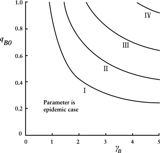
Figure 5 graphs minimum requirements on $q_{A0}$ and ${\gamma }_A$ to contain an epidemic with quarantine alone, based on setting the “late start” reproduction number $R_{\mathit{AL}}$ in Eq. (60) equal to unity. Comparing Fig. 5 to Fig. 3, we see that, to contain an epidemic of a given severity, quarantine requires less strength and less speed than does isolation. (Of course, quarantine has a much greater impact on the public.)

Fig. 5.

Conditional requirements to contain an epidemic by quarantine alone

When isolation and quarantine are combined, a pertinent issue is allocation of effort between the two. How is burden of performance to be divided? We will lay out examples of choices.

Simplicity of the reproduction number formula for isolation combined with quarantine started early makes allocation for this case an easy task. Allocation is more complicated for late quarantine start, and it is perhaps a more realistic scenario, so we devote our attention to this case.

Figures 6 and 7 quantify strength and speed of the two processes needed to contain an epidemic, on condition that the processes start early enough. For brevity, we show only results for cases II and III. Figures 6 and 7 are based on setting $R_{\mathrm{ABL}}=1$, using Eqs. (63) and (65).

Fig. 6.

Conditional requirements on isolation and quarantine combined to contain epidemic case II

Fig. 7.

Conditional requirements on isolation and quarantine combined to contain epidemic case III

It goes without saying that on-the-ground realities drive what can be done; practicalities of implementation are primary. For instance, are means in place for testing and contact tracing necessary for isolation? What is the public’s commitment to quarantine? Figures 6 and 7 provide broad-brush quantitative insight into potential of the combined measures.

Figures 8 and 9 address consequences of efforts falling short. In these figures, we arbitrarily set $q_{A0}=q_{B0}$ and ${\gamma }_A={\gamma }_B$ and called the common values $q_0$ and ${\gamma }_0$.

Fig. 8.

$s_{T\infty }$ as a function of $q_0$ for various epidemic severities, with ${\gamma }_0$ as parameter

Fig. 9.

$i_{T\mathrm{MAX}}$ as a function of $q_0$ for various epidemic severities, with ${\gamma }_0$ as parameter

Figure 8 plots $s_{T\infty }$ as a function of $q_0$ with ${\gamma }_0$ as parameter for each of the epidemic cases considered, at $p(0)={10}^{-4}$. Figure 8 shows that mitigation achieved by strength $q_0$ just above a critical value $q_{0C}$ is much greater, though short of containment, than that achieved by strength just below it. The critical strength is roughly two-thirds of the containment requirement derived from $R_{\mathit{ABL}}=1$, which we denote as $q_{0R}$. Table 3 compares $q_{0C}$ to $q_{0R}$ for the four epidemic cases, for ${\gamma }_0=4$ and $p(0)={10}^{-4}$.

Table 3.

Comparing critical value of combined strength $q_0$ to that derived from $R_{\mathrm{ABL}}=1$, when ${\gamma }_0=4$ and $p(0)={10}^{-4}$

	Case I	Case II	Case III	Case IV
$q_{0C}$	0.066522	0.124518	0.202420	0.338233
$q_{0R}$	0.0964	0.1813	0.3008	0.5329
Ratio	0.6900	0.6868	0.6729	0.6347

In Fig. 8 are bold circles marking points where a curve’s abscissa meets a containment requirement $q_{0R}$. Notice that the circles cluster at about $s_{T\infty }=$ 0.9995. These are but a few of the points that went into calculation of $d_M$ for $R_{\mathrm{ABL}}$.

For brevity, we omit graphs of quarantine alone and isolation alone in the format of Fig. 8. We can summarize important aspects of them: The graph for quarantine alone shows discontinuities similar to those in Fig. 8. The graph for isolation alone, on the other hand, has smooth, gently sloping curves. The graph of isolation alone also shows that, while $d_M$ is only 0.98590 at $p(0)={10}^{-4}$, plausibly achievable increases in $q_{B0}$ from $q_{B0R}$ values can raise $s_{T\infty }$ to much higher levels for epidemic cases I and II. In case I, e.g., with ${\gamma }_B=$ 4, increases in $q_{B0}$ from the $q_{B0R}$ value of 0.2678 to 0.320 and 0.420 raise $s_{T\infty }$ to 0.997 and 0.999, respectively. Creating graphs in the format of Fig. 8 is probably the best way to find levels of intervention effort that achieve desired $s_{T\infty }$ values when $d_M$ is too low, i.e., when intervention has begun too late.

In Fig. 8, $s_{T\infty }$ is highly sensitive to small changes in $q_0$. If $s_{T\infty }$ is a continuous function of $q_0$, then for every $\epsilon >0$ there exists a $\delta >0$ such that if $\left|\mathrm{\Delta }{q}_0\right|<\delta$ then $\left|\mathrm{\Delta }{s}_{T\infty }\right|<\epsilon$. We conducted numerical experiments at the critical $q_0$ points to quantify this. An example result: for Case III and ${\gamma }_0=4$, as $\left|\mathrm{\Delta }{q}_0\right|$ decreased from ${10}^{-3}$ to ${10}^{-6}$ $\mathrm{\Delta }{s}_{T\infty }$ decreased only from 0.24620 to 0.23521. But despite the extremely slow convergence, we believe the function is continuous and, in fact, differentiable.

As mentioned earlier, we used the Adams–Moulton (A–M) numerical integration algorithm for this study. To verify that the high sensitivity of $s_{T\infty }$ to changes in $q_0$ we see in Fig. 8 is not an artifact of the algorithm, we also used the Runge–Kutta (R–K) and backward differentiation formula (BDF) algorithms to integrate the ODEs and recreate Fig. 8. We found the same high sensitivity with all three algorithms. Furthermore, the difference between $q_{0C}$ values computed by the A–M algorithm and R–K algorithm was less than $6·{10}^{-6}$, and difference between $q_{0C}$ values computed by A–M algorithm and BDF algorithm was less than $1.3·{10}^{-5}$. Differences in computed $\mathrm{\Delta }{s}_{T\infty }$ were also minimal.

Figure 9 plots $i_{T\mathrm{MAX}}$ as a function of $q_0$ with ${\gamma }_0$ as parameter for epidemic cases III and IV. Discontinuities are again evident, at the same critical values of $q_0$. The figure shows that half measures leave the public facing a still-serious epidemic.

Expanding the Model to Examine Endemic Equilibrium States

Our final objective is to examine endemic equilibrium states. We will calculate equilibrium values for the important state variables and examine dynamics of a disease coming to equilibrium. We assume that isolation, but not quarantine, is in effect. Maintaining quarantine over a significant portion of the population for a very extended period is unlikely.

For a model to exhibit an endemic state, it must include the population’s natural dynamics: births, deaths and net immigration. It then becomes necessary for us to use, instead of probabilities, state variables $S(t)$, the expected number of people in the population susceptible but well at time $t$; $I(t)$, the expected number of people infected and not in isolation at time $t$; and $R(t)$, the expected number of people in the population who have been infected but have recovered at time $t$. We continue to assume that the number of people who die from the disease is not an appreciable fraction of the population. Denote the number of births and net immigrants per unit time, assumed constant, as $B$. Let the probability a person drawn at random from the population is dead of natural causes by time $t$ given he or she is alive at time $\tau$ be

$$\mathrm{d}(t\left|\tau )=1-exp(-{\gamma }_D(t-\tau ))\right).$$ 73

Let the rate of new infections be given by

$$P_{\mathrm{DOT}}=\beta \frac{\mathit{SI}}{S+I+R}.$$ 74

Then

$$\begin{array}{cc}& \frac{\mathrm{d}P}{\mathrm{d}t}=P_{\mathrm{DOT}}\hfill \\ \hfill & S(t)=S(0)(1-d(t\left|0\right)))+{\int }_0^t(B-P_{\mathrm{DOT}})(1-d(t\left|\tau ))\mathrm{d}\tau \right)\hfill \\ \hfill \end{array}$$ 75

$$\frac{\mathrm{d}S}{\mathrm{d}t}=B-P_{\mathrm{DOT}}-{\gamma }_{D}S.$$ 76

It is convenient to consider $R(t)$ next:

$$\begin{array}{cc}& R(t)={\int }_0^t\dot{P}(\tau )r(t\left|\tau )(1-d(t\left|\tau ))\mathrm{d}\tau \right)\right)\hfill \\ \hfill & R(t)={\int }_0^{t}P(\tau )\frac{d}{\mathrm{d}t}\left(r(t\left|\tau )(1-d(t\left|\tau ))\right)\right)\right)\mathrm{d}\tau \hfill \\ \hfill \end{array}$$ 77

which leads, via Eqs. (11) to (17), to

$$\begin{array}{cc}& R=R_1-R_2\hfill \\ \hfill & \frac{\mathrm{d}{R}_1}{\mathrm{d}t}={\gamma }_{D}P+({\gamma }_R+{\gamma }_D)(R_{11}-R_1)\hfill \\ \hfill & \frac{\mathrm{d}{R}_{11}}{\mathrm{d}t}={\gamma }_{R}P-({\gamma }_R+{\gamma }_D)R_{11}\hfill \\ \hfill & \frac{\mathrm{d}{R}_2}{\mathrm{d}t}={\gamma }_{D}P-{\gamma }_D{R}_2.\hfill \\ \hfill \end{array}$$ 78

Next, modifying Eq. (37):

$$\begin{array}{cc}& I(t)={\int }_0^t\dot{P}(\tau )(1-r(t\left|\tau ))(1-q_B(t\left|\tau ))(1-d(t\left|\tau ))\mathrm{d}\tau \right)\right)\right)\hfill \\ \hfill & I(t)=P(t)-{\int }_0^{t}P(\tau )\frac{\mathrm{d}}{\mathrm{d}\tau }\left((1-r(t\left|\tau ))(1-q_B(t\left|\tau ))(1-d(t\left|\tau ))\right)\right)\right)\right)\mathrm{d}\tau \hfill \\ \hfill \end{array}$$ 79

which can be written, in fashion similar to Eq. (38),

$$I=P-(1-q_{B0})R_1-I_B$$ 80

where, after again using Eqs. (11) to (17),

$$\begin{array}{cc}& \frac{\mathrm{d}{I}_B}{\mathrm{d}t}={\gamma }_D{q}_{B0}P+({\gamma }_R+{\gamma }_B+{\gamma }_D)(I_{B1}-I_B)\hfill \\ \hfill & \frac{\mathrm{d}{I}_{B1}}{\mathrm{d}t}=\left(\frac{{\gamma }_R^2+{\gamma }_B^2+{\gamma }_D({\gamma }_R+{\gamma }_B)}{{\gamma }_R+{\gamma }_B+{\gamma }_D}\right)q_{B0}P+({\gamma }_R+{\gamma }_B+{\gamma }_D)(I_{B2}-I_{B1})\hfill \\ \hfill & \frac{\mathrm{d}{I}_{B2}}{\mathrm{d}t}=\left(\frac{2{\gamma }_R{\gamma }_B}{{\gamma }_R+{\gamma }_B+{\gamma }_D}\right)q_{B0}P-({\gamma }_R+{\gamma }_B+{\gamma }_D)I_{B2}.\hfill \\ \hfill \end{array}$$ 81

With these equations in hand, we can proceed. If the variables $S$, $I$ and $R$ are all constant, then

$$\frac{\mathrm{d}P}{\mathrm{d}t}=P_{\mathrm{DOT}}=v$$ 82

where $v$ is a constant. Then, Eqs. (76), (78) and (81) all take the form

$$\dot{x}+\lambda x=k_{1}t-k_2$$

which has solution

$$x=\frac{1}{\lambda }\left(k_1\left(t-\frac{1}{\lambda }\right)-k_2\right).$$ 83

Using Eqs. (74), (76), (78), (80) and (81), we eventually find the steady-state values

$$\begin{array}{cc}& S_{\ast }=(B-v)/{\gamma }_D\hfill \\ \hfill & I_{\ast }=v(1-q_{B0})\left(\frac{1}{{\gamma }_R+{\gamma }_D}\right)\left(1+\frac{{\gamma }_R}{{\gamma }_R+{\gamma }_D}\right)+v{q}_{B0}\left(\frac{1}{{\gamma }_R+{\gamma }_B+{\gamma }_D}\right)·\hfill \\ \hfill & \left(1+\frac{{\gamma }_R+{\gamma }_B}{{\gamma }_R+{\gamma }_B+{\gamma }_D}+\frac{2{\gamma }_R{\gamma }_B}{{({\gamma }_R+{\gamma }_B+{\gamma }_D)}^2}\right)\hfill \\ \hfill & R_{\ast }=v\left(\frac{1}{{\gamma }_D}-\frac{1}{{\gamma }_R+{\gamma }_D}-\frac{{\gamma }_R}{{({\gamma }_R+{\gamma }_D)}^2}\right).\hfill \\ \hfill \end{array}$$ 84

Given numerical values for the parameters, one could solve for $v$ via Eq. (74). However, it is of more interest to assume ${\gamma }_D<<{\gamma }_R$, so Eqs. (84) become

$$\begin{array}{cc}& S_{\ast }=(B-v)/{\gamma }_D\hfill \\ \hfill & I_{\ast }=v{R}_B/\beta \hfill \\ \hfill & R_{\ast }=v/{\gamma }_D\hfill \\ \hfill \end{array}$$ 85

and Eq. (74) becomes

$$\begin{array}{cc}& v=\beta \left(\frac{((B-v)/{\gamma }_D)(v{R}_B/\beta )}{(B-v)/{\gamma }_D+v{R}_B/\beta +v/{\gamma }_D}\right)\hfill \\ \hfill & 1=\frac{((B-v)/{\gamma }_D)R_B}{(B/{\gamma }_D)+v(R_B/\beta )}.\hfill \\ \hfill \end{array}$$ 86

We can then solve for $v$ in closed form and find, with ${\gamma }_D<<\beta$,

$$\begin{array}{cc}& v=B\left(\frac{R_B-1}{R_B}\right)\hfill \\ \hfill & S_{\ast }=\left(\frac{B}{{\gamma }_D}\right)\left(\frac{1}{R_B}\right)\hfill \\ \hfill & I_{\ast }=\left(\frac{B}{\beta }\right)(R_B-1)\hfill \\ \hfill & R_{\ast }=\left(\frac{B}{{\gamma }_D}\right)\left(\frac{R_B-1}{R_B}\right)\hfill \\ \hfill \end{array}$$ 87

where $R_B$ is the isolation reproduction number given by Eq. (54). Note that the threshold for an endemic state in an epidemic with isolation is $R_B>1$. Although the probabilistic model has the added complexities of a second-order removal probability and an isolation process, it has led to the well-known SIR equations for the equilibrium state, with $R_B$ replacing $R_0$. (See, e.g., Diekmann et al. 2013.)

How does a disease become endemic? Only under special conditions, it appears. The disease must first have been epidemic, to drive the number of susceptible people below $S_{\ast }$. The equilibrium position is at the threshold for herd immunity, when the portion of the population immune to the disease suffices to negate an epidemic. (See, e.g., Hethcote 2000.) If an incursion of infected people occurs when $S>S_{\ast }$ and mitigation is inadequate, an epidemic inevitably follows, driving $S$ past $S_{\ast }$ to the $S_{\infty }$ concomitant with the starting point and $I$ to zero. Then $S$ begins a disease-free course to the natural capacity $B/{\gamma }_D$.

If the disease incursion occurs when $S$ is well below $S_{\ast }$, the outbreak is relatively quickly extinguished and $S$ continues its path to $B/{\gamma }_D$. Only if the incursion happens as $S$ nears $S_{\ast }$ from below, as in Fig. 10, can the S trajectory be forced into transition to its equilibrium value.

Fig. 10.

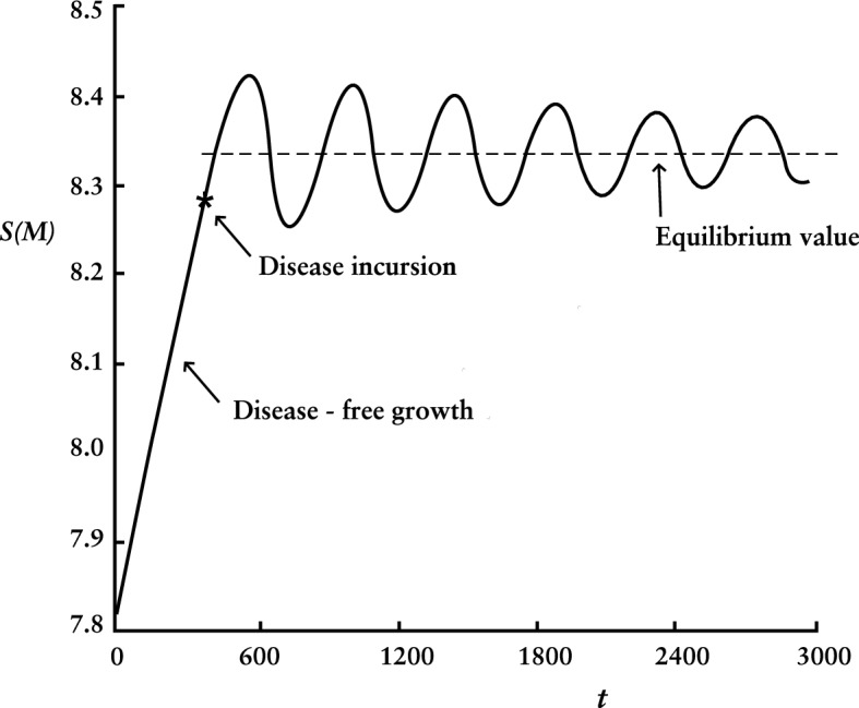
Expected number of people susceptible but well as a function of time as disease settles into endemic equilibrium state

Figure 10 pictures dynamics of settling into equilibrium. Here, the natural capacity $B/{\gamma }_D={10}^7$, ${\gamma }_D=1/1500$, $q_{B0}=0.5$, ${\gamma }_B=4$ and other values are as in Sect. 6. If the average recovery period is 2.6 weeks, then 20 time units equal one year.

Compared to duration of an epidemic, dynamics of settling into equilibrium are slow, as is well known. (See, e.g., analysis of the linearized SIR model in Diekmann et al. 2013.) For $R_B=1.2$, as in Fig. 10, the oscillation period is about 21 years and decay time constant about 140 years. For $R_B=2$, they are about 9 and 90 years.

The equilibrium $I_{\ast }$ is small compared to the epidemic $I_{\mathit{MAX}}$: 78 people for $R_B=1.2$ and 235 for $R_B=2$. Transitioning as in Fig. 10, amplitude of oscillations in $S$ and $R$ depends on $R_B$ and imperceptibly (if at all, given numerical uncertainty) on size of the small incursion or its timing (within limits described earlier).

Computed values agree with Eq. (87) to within small fractions of a percent.

Concluding Remarks

We review here main points of this article, summarize how the probabilistic model differs from other models in the literature and opine on advantages and disadvantages these differences confer.

Beginning with a small but nontrivial difference, the probabilistic model adopts a second-order gamma distribution for removal probability while most other models employ one of first order. The first-order distribution is attractive for its simplicity but is unrealistic in its time profile. In concert with the mass action law, the second-order removal distribution predicts an expected maximum fraction of population infected at any one time, $i_{\mathit{MAX}}$, significantly greater than does the first order, e.g., more than 30% for $R_0<2.75$. This is consequential for predicting peak stress on medical facilities.

Our numerical studies indicate that the limit of the ratio of $i_{\mathit{MAX}}$ produced by the gamma distribution of order $n$ to that of order one is $2n/(n+1)$ as $R_0$ goes to one.

Moving to a more significant difference, the probabilistic model incorporates two parameters versus one in both isolation and quarantine. We believe that modeling both strength ($q_{A0}$ and $q_{B0}$) and speed ($\gamma {}_A$ and ${\gamma }_B$) of these processes is framework for more realistic representation. These parameters are easy to interpret and potentially measurable, which should make the model useful in empirical research. When quarantine or combined intervention strength is modeled, we discover that intervention effectiveness, as measured by either $s_{T\infty }$ or $i_{\mathit{TMAX}}$, is highly sensitive to small changes at a critical value of that strength. The critical value is about two-thirds of the containment requirement derived from reproduction number. Does this accurately model the natural world? If so, knowledge of the phenomenon should be valuable.

Another major difference is that our model is founded on first principles of probability rather than mathematical simplicity. Coefficients such as $2{\gamma }_R{\gamma }_B/({\gamma }_R+{\gamma }_B)$ that arise naturally in the probabilistic model have no counterpart in typical SIR-like models. Note that the coefficient combines parameters from different processes. The typical SIR-like model describes transitions with pairs of equations like ${\dot{x}}_i=-{\gamma }_{\mathit{ij}}{x}_i+...$ and ${\dot{x}}_j={\gamma }_{\mathit{ij}}{x}_i+...$, where the rate ${\gamma }_{\mathit{ij}}$ common to the pair is a parameter set by the analyst. Whether basis in probability is an advantage remains to be seen. We expect it to represent reality more accurately, but comparison with field data is required.

A disadvantage: the ODE equations modeling quarantine are not time-invariant, which can be a hindrance, e.g., in stability analysis. We have modeled quarantine as time-driven, which we believe is more realistic than event-driven, e.g., removal only after tracing from contact with an infectious person.

We used reproduction numbers to determine requirements on $q_{A0}$, $q_{B0}$, ${\gamma }_A$ and ${\gamma }_B$ to contain epidemics of varying severity, confirmed them with ODE results and quantified dependence of intervention effectiveness on when interventions begin. We derived expressions for endemic disease equilibria when affected by isolation and found familiar formulas, with $R_B$ replacing $R_0$. We examined dynamics of coming to an equilibrium and found that only special conditions permit it.

In sum, assuming a homogeneous population we developed a model based on first principles of probability, with eight differential equations, six parameters and five reproduction numbers, and quantified important aspects of isolation and quarantine effectiveness in controlling an epidemic.

Funding

Not applicable.

Declarations

Conflict of interest

The author declares no conflict of interest.

References

- Abbey H. An examination of the Reed-Frost theory of epidemics. Hum Biol. 1952;243:201. [PubMed] [Google Scholar]
- Anderson D, Watson R. On the spread of a disease with gamma distributed latent and infectious periods. Biometrika. 1980;67(1):191–198. doi: 10.1093/biomet/67.1.191. [DOI] [Google Scholar]
- Bernoulli D. An attempt at a new analysis of the mortality caused by smallpox and the advantages of inoculation to prevent it. Mem Math Phys Acad Roy Sci Paris. 2004;14:275. doi: 10.1002/rmv.443. [DOI] [PubMed] [Google Scholar]
- Blower S. An attempt at a new analysis of the mortality caused by smallpox and the advantages of inoculation to prevent it. Rev Med Virol. 2004;14:275. doi: 10.1002/rmv.443. [DOI] [PubMed] [Google Scholar]
- Brauer F. Mathematical epidemiology: past, present and future. Infect Dis Model. 2017;2(2):113–127. doi: 10.1016/j.idm.2017.02.001. [DOI] [PMC free article] [PubMed] [Google Scholar]
- Castillo-Chavez C, Castillo-Garsow CW, Yakuba A. Mathematical models of isolation and quarantine. JAMA. 2003;290(21):2876–2877. doi: 10.1001/jama.290.21.2876. [DOI] [PubMed] [Google Scholar]
- Colizza V, Barrat A, Barthelemy M, Valleron A, Vespignani A. Modeling the worldwide spread of pandemic influenza: baseline case and containment interventions. PLoS Med. 2007;4:e13. doi: 10.1371/journal.pmed.0040013. [DOI] [PMC free article] [PubMed] [Google Scholar]
- Day T, Park A, Madras N, Gumel A, Wu J. When is quarantine a useful control strategy for emerging infectious diseases? Am J Epidemiol. 2006;163(5):479–485. doi: 10.1093/aje/kwj056. [DOI] [PMC free article] [PubMed] [Google Scholar]
- De Maia JO. Some mathematical developments on the epidemic theory developed by Reed and Frost. Hum Biol. 1952;24(3):167. [PubMed] [Google Scholar]
- Denes A, Gumel AB. Modeling the impact of quarantine during an outbreak of Ebola virus disease. Infect Dis Model. 2019;4:12–27. doi: 10.1016/j.idm.2019.01.003. [DOI] [PMC free article] [PubMed] [Google Scholar]
- Diekmann O, Heesterbeek H, Britton T. Mathematical tools for understanding infectious disease dynamics. Princeton: Princeton University Press; 2013. [Google Scholar]
- Feng ZI, Thieme HR. Endemic models with arbitrarily distributed periods of infection. SIAM J Appl Math. 2000;61(3):803–833. doi: 10.1137/S0036139998347834. [DOI] [Google Scholar]
- Ferguson NM, Cummings DAT, Fraser C, Cajka JC, Cooley PC, Burke DS. Strategies for mitigating an influenza epidemic. Nature. 2006;442:448–452. doi: 10.1038/nature04795. [DOI] [PMC free article] [PubMed] [Google Scholar]
- Fraser C, Riley S, Anderson R, Ferguson N. Factors that make an infectious disease controllable. PNAS. 2004;101(16):6146–6151. doi: 10.1073/pnas.0307506101. [DOI] [PMC free article] [PubMed] [Google Scholar]
- German TC, Kadau K, Longini IM, Macken CA. Mitigation strategies for pandemic influenza in the US. PNAS. 2006;103(15):5935–5940. doi: 10.1073/pnas.0601266103. [DOI] [PMC free article] [PubMed] [Google Scholar]
- Gumel AB, et al. Modeling strategies for controlling SARS outbreaks. Proc R Soc Lond B. 2004;271:2223–2232. doi: 10.1098/rspb.2004.2800. [DOI] [PMC free article] [PubMed] [Google Scholar]
- Hamer WH (1906) Epidemic disease in England—the evidence of viability and of persistence. Lancet 167
- Halloran ME, et al. Modeling target layered containment of an influenza epidemic in the US. PNAS. 2008;105(12):4639–4644. doi: 10.1073/pnas.0706849105. [DOI] [PMC free article] [PubMed] [Google Scholar]
- Heesterbeck JAP, Roberts MG. How mathematical epidemiology became a field of biology. Philos Trans R Soc. 2015;370:20140307. doi: 10.1098/rstb.2014.0307. [DOI] [PMC free article] [PubMed] [Google Scholar]
- Hethcote HW. The mathematics of infectious disease. SIAM Rev. 2000;42(4):599–653. doi: 10.1137/S0036144500371907. [DOI] [Google Scholar]
- Hethcote H, Zhein M, Shengbing I. Effects of quarantine in six endemic models for infectious diseases. Math Biosci. 2002;180:141–160. doi: 10.1016/S0025-5564(02)00111-6. [DOI] [PubMed] [Google Scholar]
- Kermack WO, McKendrick AG. A contribution to the mathematical theory of epidemics. Proc R Soc A. 1927;115(772):701–722. [Google Scholar]
- Kurtz TG. Approximation of population processes. New York: SIAM; 1981. [Google Scholar]
- Li F, Meng X, Wang X (2018) Analysis and numerical simulations of a stochastic SEIQR epidemic system with quarantine-adjusted incidence and imperfect vaccination. Special issue: Multiscale computational models for respiratory aerosol dynamics with medical applications. Comput Math Methods Med 2018 [DOI] [PMC free article] [PubMed]
- Lessler J, Cummings DA. Mechanistic models of infectious disease and their impact on public health. Am J Epidemiol. 2016;183(5):415–422. doi: 10.1093/aje/kww021. [DOI] [PMC free article] [PubMed] [Google Scholar]
- Lewis B et al (2007) Simulated pandemic influenza outbreaks in Chicago. Virginia Bioinformatics Institute, Virginia Polytechnic Institute and State University, Tech Report NDSSL-TR-07-004
- Ma J, Earn DJD. Generality of the final size formula for an epidemic of a newly invading infectious disease. Bull Math Biol. 2006;68:679–702. doi: 10.1007/s11538-005-9047-7. [DOI] [PMC free article] [PubMed] [Google Scholar]
- Sahu GP, Dhar J. Dynamics of an SEQIHRS epidemic model with media coverage, quarantine and isolation in a community with pre-existing immunity. JAMA. 2015;421(2):1651–1672. doi: 10.1016/j.jmaa.2014.08.019. [DOI] [PMC free article] [PubMed] [Google Scholar]