Abstract
Purpose:
To investigate whether a deep learning-based (DL) approach can be used for frequency-and-phase correction (FPC) of MEGA-edited MRS data.
Methods:
Two neural networks (one for frequency, one for phase) consisting of fully connected layers were trained and validated using simulated MEGA-edited MRS data. This DL-FPC was subsequently tested and compared to a conventional approach (spectral registration, SR) and to a model-based implementation (mSR) using in vivo MEGA-edited MRS datasets. Additional artificial offsets were added to these datasets to further investigate performance.
Results:
The validation showed that DL-based FPC was capable of correcting within 0.03 Hz of frequency and 0.4° of phase offset for unseen simulated data. DL-based FPC performed similarly to SR for the unmanipulated in vivo test datasets. When additional offsets were added to these datasets, the networks still performed well. While SR accurately corrected for smaller offsets, it often failed for larger offsets. The mSR algorithm performed well for larger offsets, which was due to the model being generated from the in vivo datasets. In addition, the computation times were much shorter using DL-based FPC or mSR compared to SR for heavily distorted spectra.
Conclusion:
These results represent a proof of principle for the use of DL for preprocessing MRS data.
Keywords: edited MRS, frequency correction, phase correction, deep learning, MEGA-PRESS
1. Introduction
Magnetic resonance spectroscopy (MRS) is a non-invasive method for metabolite quantification that is used in a variety of clinical research applications1. However, scanner frequency drift, subject motion or other instabilities may result in frequency and phase shifts of individual transients, which in turn can lead to line-broadening and signal loss upon averaging2. Therefore, frequency-and-phase correction (FPC) of individual transients is an essential data processing step in order to allow for reliable quantification of the targeted metabolites. Appropriate FPC is even more crucial when using J-difference-edited MRS methods3 such as MEGA-PRESS4-7, which relies on subtraction of two spectra containing strong signals (OFF and ON) in order to reveal a much smaller targeted signal (e.g., GABA) in the resulting difference spectrum. Misaligned OFF and ON spectra within a dataset lead to subtraction artifacts in the resulting difference spectrum, which can bias subsequent quantification8.
Several approaches for FPC have been proposed, including frequency alignment based on peaks within the spectra9,10, automated alignment using correlation of spectral windows11, FPC based on cross-correlation and fitting algorithms12, and time-domain spectral registration13. All of these approaches rely upon the common information content of each transient in order to achieve alignment. There is often an implicit assumption that the only way in which individual transients of the same acquisition differ is by some (small) frequency and phase shifts. The signal-to-noise ratio (SNR) of individual transients is a function of voxel size, acquisition geometry and water suppression quality, and FPC becomes increasingly challenging for low SNR data. Moreover, subject motion often leads to changes in the quality of water suppression and/or excitation of subcutaneous lipid signals, resulting in artifacts that violate the assumptions of FPC and bias results14,15.
Deep learning (DL) is a popular strategy to address a wide range of computational problems, relying upon a multi-layer network with a large number of weights and bias parameters that are optimized during network training16. Recent technical advances in processor speed and memory capacity are crucial in allowing for sufficient network training within a reasonable time. The structure of the network, in terms of number of layers and functions, is fixed prior to optimization, and needs to be sufficiently complex to extract the required information from input data while avoiding simultaneously overfitting. Networks are trained using a set of data for which the true output values are known. After training, the network is validated and tested on data that were not used for training.
DL is an effective image processing approach, which has been enthusiastically adopted in MR imaging but has had a more modest impact on MRS so far. DL has been applied to the image domain of MRSI to deliver resolution enhancement of metabolite maps17. In the spectral domain, DL has previously been implemented for metabolite quantification18, measurement uncertainty estimation19, spectral reconstruction20, and artifact elimination21,22. DL algorithms have been shown to perform especially well in low-SNR applications, suggesting DL may be particularly suitable for single-transient FPC for edited MRS. The main aim of this paper was to investigate whether DL can be used for FPC of MEGA-edited MRS data. Networks for FPC were trained and validated using simulated data and further tested using in vivo MEGA-edited MRS data from the openly available Big GABA repository23,24.
2. Methods
2.1. Data Selection and Simulation
Data selection for sufficient network training is one of the major challenges in deep learning. Using in vivo MRS datasets to train an FPC network would rely on another FPC method in order to identify the “true” frequency and phase offsets for each spectrum. Since the true offsets for each transient are unknown for in vivo data, in this work training/validation transients were simulated with an appearance similar to in vivo spectra. In order to establish in vivo-like levels of SNR and residual water signal, data from the publicly available Big GABA repository23 were used, which includes a total of 101 Philips MEGA-edited datasets collected from 9 different sites (3 T field strength, TE = 68 ms, 2048 data points sampled at 2 kHz spectral width, 320 transients, https://www.nitrc.org/projects/biggaba/). Since there were minor acquisitional differences between the sites, only data from sites P1, P3, and P9 were selected (N = 33), all of which were acquired using a water suppression method (VAPOR25) that generated a positive water residual in the spectra. Data collection was conducted in accordance with ethical standards set by the institutional review board at each site, and written informed consent was obtained from each participant.
MEGA-PRESS training/validation transients were simulated in the FID-A toolbox26, using ideal excitation/refocusing pulses and shaped editing pulses. The main simulation parameters were set according to the acquisition parameters used in the Big GABA project23 (15-ms sinc-Gaussian editing pulses with FWHM = 88.5 Hz, 2048 data points sampled at 2 kHz spectral width) and a total of 14 metabolites (Asp, Cr, GABA, Gln, Glu, GPC, GSH, Ins, Lac, NAA, NAAG, PCh, PCr, Scyllo) and a positive water residual signal were included in the simulated spectra. The simulated signal intensities and linewidths were appropriately set in order to match those in the in vivo datasets. The simulated in vivo OFF and ON transients were each duplicated 20,500 times (with 40,000 ON+OFF spectra allocated for training and 1,000 for validation), and random complex Gaussian noise was added to each at a level that matched a single in vivo transient, i.e., the standard deviation of the spectral signal between 10 and 11 ppm.
2.2. Network Implementation and Training
Frequency correction and phase correction are separable problems, implemented as sequential (frequency first, then phase) networks handling the frequency-domain spectra of individual transients (Figure 1). Each network consisted of an input layer with 1024 nodes, followed by two hidden fully connected (FC) layers with 1024 and 512 nodes, respectively, and a final FC linear output layer with one node. Each of the hidden FC dense layers was followed by a rectified linear unit (ReLu) activation function, which allows the introduction of non-linearity in the network. The output from each network was the predicted offset, either the frequency offset determined in Hz or the phase offset determined in degrees. These two networks were implemented and trained using the TensorFlow framework in Python with a 2.3 GHz Intel Core i5 CPU.
Figure 1.
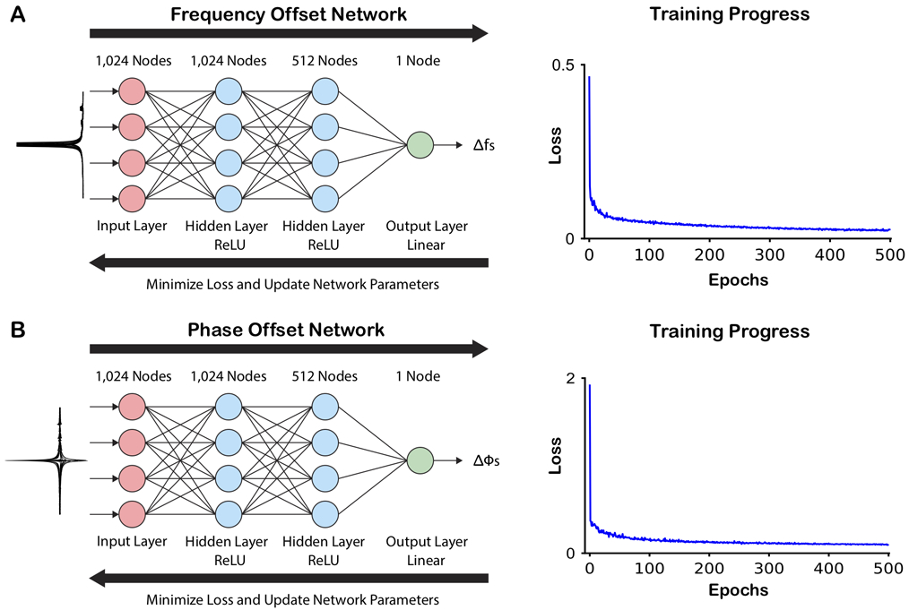
Network structure and training progress. Both the frequency (A) and phase (B) offset networks have the same basic structure with three fully connected (FC) layers (1024, 512, 1 node(s)). The two hidden FC layers were each followed by a rectified linear unit (ReLU) activation function, and the output FC layer was followed by a linear activation function, which generated the output offset as a continuous variable. Simulated spectra manipulated with frequency offsets or phase offsets were used as training data for the respective network (illustrated on the left-hand of the figure). During the training, the loss between the predicted frequency/phase offsets and the true applied offsets were minimized, and the network parameters updated. Each network was trained through 500 epochs.
In order to generate the training set, the simulated transients were manipulated with uniformly distributed frequency and phase offsets. The frequency offset network was trained using the spectral representations of the 40,000 transients in magnitude mode (so as to be blind to phase errors). Artificial frequency offsets in the range of −20 to 20 Hz were applied to each transient, and these frequency offsets defined as target output. Artificial phase offsets in the range of −90° to 90° were applied to the 40,000 training transients, which were input to the phase offset network as real-only spectra (without frequency offsets), with the artificial phase offsets as target output.
Prior to input into a network, each manipulated training spectrum was normalized to the maximum signal in the spectrum (the residual water signal), and the central 1024 points were selected (i.e., 0.8 – 8.6 ppm) in order to prevent overfitting of noise at the frequency limits of the spectra, and to reduce training time. Consequently, the total number of spectral samples matched the number of nodes in the input layer of the networks. Individual training of both networks was conducted using the Adam algorithm27 to optimize the network parameters with a constant learning rate of 0.01 for 500 epochs, with a batch size of 64, and mean absolute error as the loss function.
2.3. Validation and Test of the Networks
Artificial offsets distributed uniformly over the intervals of −20 to 20 Hz and −90° to 90° were shuffled into random pairs consisting of one unique frequency offset and one unique phase offset, and then applied to each simulated validation transient in the time domain, which generated a wide range of misaligned transients to validate the networks. Figure 2 illustrates how the validation and test of the networks were performed. First, the uncorrected data were Fourier transformed, individually normalized to the maximum signal in the spectrum, and the central 1024 samples of the magnitude spectra were extracted and used as input to the trained frequency offset network. The resulting predicted frequency offset (Δf) was then applied to frequency-correct the original transient in the time domain. Second, this frequency-corrected validation transient was then Fourier transformed, normalized, and the central 1024 samples of the real spectrum were extracted and used as input to the trained phase offset network. The resulting predicted phase offset (Δϕ) was then used to phase-correct the frequency-corrected transient. Finally, all fully corrected FIDs were used to compute an average difference spectrum by subtracting the corrected OFF spectra from the corrected ON spectra.
Figure 2.
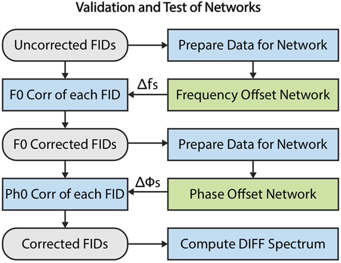
Workflow illustrating the validation and test of the networks. First, the uncorrected FIDs were prepared (FFT, normalize, crop, magnitude) and input to the frequency offset network. The predicted frequency offset (Δf) was applied to each FID. Second, these frequency-corrected FIDs were then prepared (FFT, normalize, crop, real) and input to the phase offset network. The predicted phase offset (Δϕ) for each FID was subsequently used to phase correct the frequency-corrected FIDs. An average difference spectrum was computed by subtracting the averaged OFF spectrum from the average ON spectrum.
The same process was also used to investigate the network performances when tested with offsets beyond the trained ranges (−40 to 40 Hz and −180° to 180°). In addition, the network performances were also tested for transients simulated as described previously, but with different amounts of residual water signal ranging from 0 to twice the residual water intensity used in the training data.
2.3.1. In Vivo Tests
The 33 selected in vivo datasets were used for testing the trained and validated networks. The DL-corrected difference spectra were compared to the difference spectra computed using spectral registration13 (SR), as implemented in Gannet28. The SR algorithm was performed in the time-domain, and ON and OFF transients were registered to a single template. In the registration process, only the first n points of the signal were used, where n was the last point where the SNR was > 3, where the noise was computed from the last 25% of the time-domain signal. n was limited to be at least 100. The real and imaginary parts of the first n points of each transient were then concatenated as a real vector, to be registered to the median transient of the dataset using the nlinfit function in MATLAB. The fitted parameters from one transient was used as starting parameters for the subsequent transient in the dataset. The initial starting values for the offsets were 0 Hz and 0 degrees. After registration, the transients were averaged, and global frequency and phase correction was performed using creatine/choline (Cr/Cho) modeling (nlinfit) of this averaged spectrum in order to correct for the residual frequency and phase offsets.
A model-based version of SR (mSR) was also implemented to offer a prior-knowledge analog to the DL algorithm. This mSR algorithm differs from SR by using a noise-free model as the template, instead of the median transient of the dataset. Noise-free ON and OFF FID models were created in Osprey29, an open-source MATLAB toolbox, following peer-reviewed pre-processing recommendations1. All 33 datasets were loaded (OspreyLoad), pre-processed (OspreyProcess), and modelled with a frequency-domain linear-combination algorithm (OspreyFit). During the pre-processing, the metabolite data were eddy-current corrected30 with the unsuppressed water data. Prior to averaging, the individual transients were frequency-and-phase corrected using robust spectral registration, and the residual water was removed with a Hankel singular value decomposition (HSVD) filter31. The removed water frequency components were stored for further use. Linear-combination modelling of the ON and OFF spectra was performed separately for each sub-spectrum between 0.5 and 4.0 ppm. The basis set included 19 metabolite (ascorbate, aspartate, creatine (Cr), negative creatine methylene (-CrCH2), GABA, glycerophosphocholine (GPC), glutathione, glutamine, glutamate (Glu), water, myo-inositol (mI), lactate, N-acetylaspartate (NAA), N-acetylaspartylglutamate, phosphocholine, phosphocreatine, phosphoethanolamine, scyllo-inositol, and taurine) and 8 lipid/macromolecule resonances (MM0.94, MM1.22, MM1.43, MM1.70, MM2.05, Lip09, Lip13, Lip20). The modelling included zero-filling by a factor of two, frequency referencing, a reduced model (NAA, Cr, GPC, Glu, and mI) to estimate initial parameter guesses, and a final model with the whole basis set. The model estimates were extracted including the whole spectral width, normalized by the NAA amplitude, and averaged. Similarly, the HSVD removed water components were normalized, averaged, and added to the Fourier-transformed models. The noise-free ON and OFF model FIDs were exported with a number of datapoints matching the in vivo data.
In addition, since the high quality of the in vivo datasets generally only required minor frequency and phase corrections, additional artificial offsets were added to the data in order to test network performance in more extreme cases. Three different amounts of additional offsets were added, first in the interval of ∣Δf∣ ≤ 5 Hz and ∣Δϕ∣ ≤ 20°, second in the interval of 5 ≤ ∣Δf∣ ≤ 10 Hz and 20° ≤ ∣Δϕ∣ ≤ 45° and third in the interval of 10 ≤ ∣Δf∣ ≤ 20 Hz and 45° ≤ ∣Δϕ∣ ≤ 90°. These offsets were all uniformly distributed and added as random pairs of frequency and phase to each transient.
2.4. Statistics and Quality Measurements
In the validation step where the true offsets were known, the mean error between the predicted and the true offsets was used to determine how well each network performed. In addition, the residual between the predicted and the true difference spectrum was also computed. For the in vivo datasets, the within-dataset (i.e., across the 320 transients) correlations of the resulting frequency and phase offsets computed using SR and DL were computed to determine overall agreement between the methods. Furthermore, a performance score defined as was used in order to determine which method (DL or SR) that performed better in terms of alignment of the in vivo data, where σ2 is the variance of the choline subtraction artifact (between 3.15 and 3.285 ppm) in the average difference spectrum. A performance score greater than 0.5 indicates that DL performed better than SR, a score less than 0.5 indicates that DL performed worse, and a score equal to 0.5 indicates that the two methods performed equally. The same quality metric was also used to compare mSR to the conventional SR algorithm.
3. Results
Training of each network was successfully carried out in ~4 hours on a 2.3 GHz CPU. To frequency-and-phase-correct one transient using the networks took ~1.4 ms, compared to spectral registration that took ~4.5 ms per transient for the unmanipulated in vivo data.
3.1. Validation
Figure 3 illustrates the results when the 1000 unseen validation transients (500 ON, 500 OFF) manipulated with a wide range of frequency and phase offsets were corrected using the networks. The predicted offsets were almost identical to the true actual offsets. The mean frequency offset error was 0.00 ± 0.03 Hz and is plotted against the correct value in Figure 3A. The mean phase offset error was −0.11 ± 0.25° and is plotted against the correct value in Figure 3B. It can be seen that the errors are generally larger at the limits of the frequency and phase ranges. There is a more apparent pattern of errors for the frequency offsets. The average DL-corrected difference spectrum arising from these 1000 transients was visually indistinguishable from the difference spectrum corrected by the true offsets.
Figure 3.
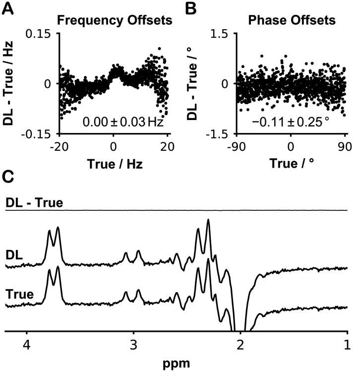
Validation of the networks. A) Plot of the error in DL-predicted frequency offset against the true offset. The mean error was 0.00 ± 0.03 Hz. B) Plot of the error in DL-predicted phase offset against the true offset. The mean error was −0.11 ± 0.25 degrees. C) The average DL-corrected difference spectrum was very similar to the true difference spectrum, as shown by the flat subtraction spectrum.
Figure 4 illustrates the results from correcting offsets beyond the trained ranges. None of the networks corrected well beyond their trained range (Figure 4A-B). An approximately linear error pattern emerged for the frequency offsets network, while a non-linear error was observed for the phase offset network. When varying the water residual intensity without adding any offsets to the data (true values were 0 Hz and 0°), network performance remained stable and accurate for water intensities greater than the trained value (Figure 4C-D). However, as the residual water intensity approached 0, both networks began to fail rapidly. Note that the simulated data had a large water residual compared to the other metabolites in the spectrum (total creatine intensity at 3 ppm was approximately 5% of the water residual intensity), which matched the in vivo data. In addition, the water residual was always positive and generally in phase with the data.
Figure 4.
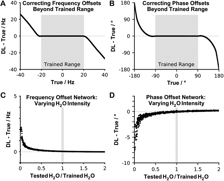
Investigation of network performance for frequency and phase offsets and residual water signal intensities outside the training conditions. A-B) Testing the networks using frequency and phase offsets beyond the trained range. C-D) Testing the networks using different amounts of water residual, varying the intensity between 0 to twice the intensity used in the training data, while both the frequency and phase offsets were set to 0 Hz and 0 degrees.
3.2. In Vivo Testing
The 33 in vivo datasets selected as test data were used as input to the trained networks. The high quality of the datasets is evident in Figure 5, where representative transients (number 80 from 160 transients per dataset) from each of the 33 datasets are shown.
Figure 5.
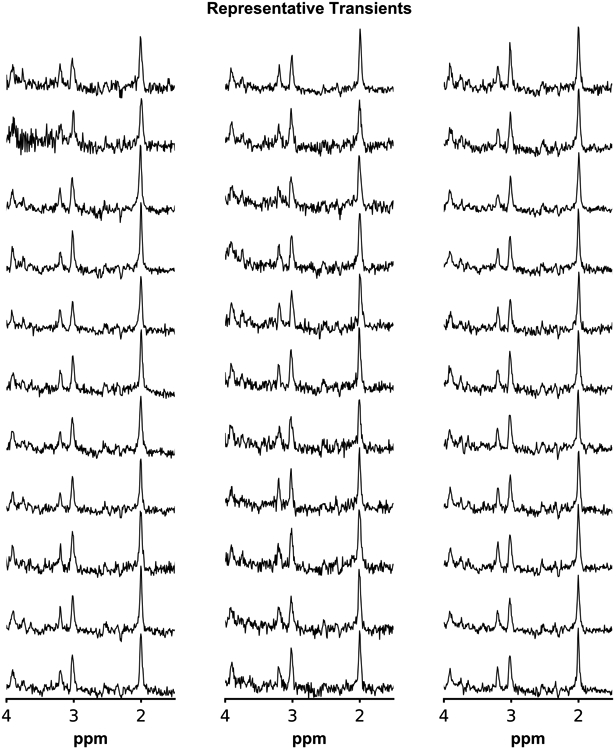
Representative single transients (center OFF, 80/160) from each of the 33 in vivo datasets.
Since there were no true offsets known for the in vivo data, the network offset predictions were compared to the resulting offsets estimated by SR. Figure 6 depicts the correlation between the resulting offsets computed using SR and DL, with each dataset shown in a distinct color. Within each dataset, a positive correlation was observed with a mean R2 of 0.997 for frequency offsets and a mean R2 of 0.906 for phase offsets between SR and DL. It can be seen in Figure 6 that there is better agreement between SR and DL with regard to frequency offsets than phase offsets, with SR-predicted phase offsets showing a markedly wider range than the DL-predicted values.
Figure 6.
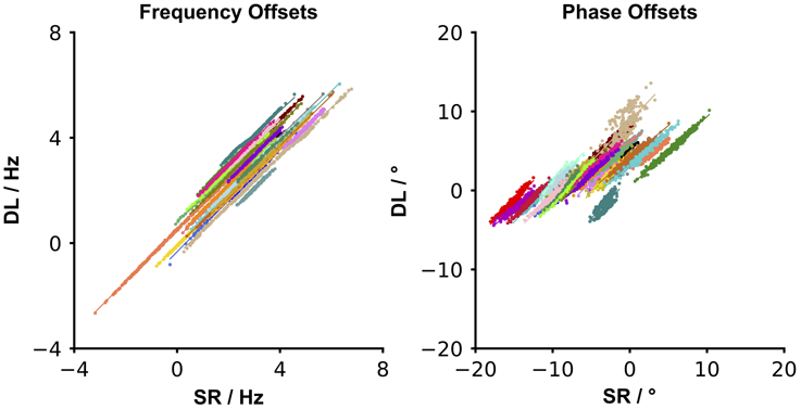
In vivo testing: DL-predicted offsets plotted against SR-predicted offsets for the 33 in vivo datasets (one point per transient; each dataset plotted in a distinct color). A high positive within-dataset correlation was observed between the methods for both the resulting frequency and phase offsets.
The resulting 33 difference spectra are plotted in the first column of Figure 7A, computed using no correction, DL-based correction, SR-based correction, and model-based mSR correction. Note that for these high-quality data, the level of subtraction artifacts seen without correction is relatively low, although Cr and Cho subtraction artifacts can be seen in some datasets. As expected, all correction approaches reduced the appearance of subtraction artifacts and improved the alignment of the difference spectra to one another. There were no large differences observed between DL and SR, as indicated by the performance scores Q (DL performed better than SR in 21/33 datasets, with a mean score = 0.51 ± 0.09, Figure 7B). The same results were observed between DL and mSR (DL performed better than mSR in 15/33 datasets, with a mean score = 0.49 ± 0.12, Figure 7C), and between mSR and SR (mSR performed better than SR in 19/33 datasets, with a mean score = 0.52 ± 0.10, Figure 7D).
Figure 7.
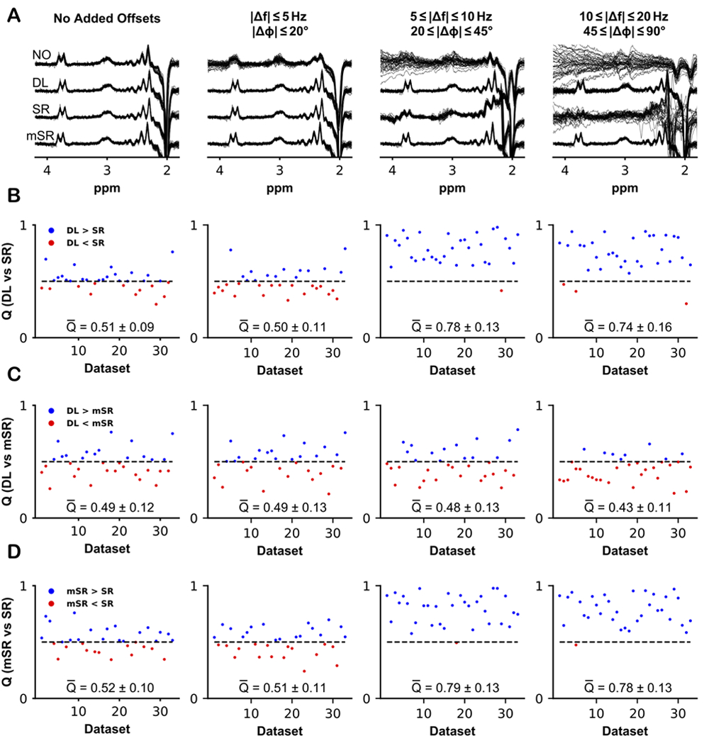
Difference spectra and performance scores comparing DL to SR, DL to mSR, and mSR to SR, for the 33 in vivo datasets. The difference spectra were either computed without any FPC (NO), using the workflow in Figure 2 (DL), using spectral registration (SR), or using model-based SR (mSR). A) Results of applying corrections to the in vivo data without further manipulation, and with additional frequency and phase offsets applied to the same 33 datasets: small offsets (0–5 Hz; 0–20°); medium offsets (5–10 Hz; 20–45°); and large offsets (10–20 Hz; 45–90°). B) Comparative performance scores Q for DL and SR for each dataset. A score above 0.5 indicated that DL performed better than SR meanwhile a score below 0.5 indicated that SR performed better than DL in terms of alignment. Q-bar indicates the mean Q score ± the standard deviation. C) Comparative Q scores for DL and mSR. D) Comparative Q scores for mSR and SR.
3.2.1. Adding Additional Offsets
Additional artificial offsets were also added to these 33 in vivo datasets (column 2-4), with the resulting spectra plotted in Figures 7A, for no correction, DL-based correction, SR-based correction, and mSR-based correction. The performance of DL and SR was comparable when small offsets were added to the data, with DL performing better than SR in 14/33 datasets and a mean performance score of 0.50 ± 0.11 (Figure 7B second column). For medium offsets, i.e., frequency offsets of 5–10 Hz and phase offsets of 20–45°, DL outperformed SR. Here, DL performed better in 32/33 datasets with a mean score of 0.78 ± 0.13 (Figure 7B third column). DL-corrected spectra for small and medium offsets do not look noticeably different from the original spectra seen in the first column in Figure 7A. For frequency offsets of 10–20 Hz and phase offsets of 45–90°, DL performed better than SR in 30/33 datasets with a mean score of 0.74 ± 0.16 (Figure 7B fourth column). It can be seen that for these larger offsets, the DL-corrected spectra start to diverge from the spectra without added offsets although they are still recognizable, while the uncorrected and SR spectra are not.
The performance of DL and mSR were similar for smaller added offsets (DL performed better than mSR in 17/33 datasets with a mean score of 0.49 ± 0.13, Figure 7C second column), and medium added offsets (DL performed better than mSR in 14/33 datasets with a mean score of 0.48 ± 0.13, Figure 7C third column). However, for larger added offsets the performance of mSR was better than DL (DL performed better than mSR in 8/33 datasets with a mean score of 0.43 ± 0.11, Figure 7C fourth column), which was evident in the resulting difference spectra in Figure 7A.
The same pattern as seen for the DL vs SR comparison was observed when comparing mSR to SR, where for small added offsets, mSR performed better than SR in 17/33 datasets with a mean score of 0.51 ± 0.11 (Figure 7D second column). When both medium and large offsets were added to the data (Figure 7D third and fourth column), mSR performed better than SR in 32/33 datasets with a mean score of 0.79 ± 0.13 and 0.78 ± 0.13, respectively.
In terms of processing duration, SR generally took much longer (~45 ms per transient) to perform with higher offsets added to the data, whereas no change in computation time was observed using DL or mSR.
4. Discussion
Frequency and phase correction are essential steps when analyzing edited MRS data in order to allow for robust quantification of the resulting difference spectra, which otherwise can be biased by subtraction artifacts. The DL-based algorithm for FPC performed similarly to SR for the unmanipulated in vivo test data, as indicated by a mean performance score of 0.5. When additional offsets were added to these datasets, DL still performed well while SR accurately corrected for smaller offsets but often failed when larger offsets were added. Not only were the resulting mean performance scores better using DL for medium and large offsets, but the computation times were also much shorter for heavily distorted spectra. The model-based SR did not show any of the disadvantages that SR experienced for our heavily distorted data. Being based on the 33 selected datasets, it may not be generally applicable, but merits further investigation.
4.1. Methodological Considerations
Many methodological options were considered before selecting the DL approach presented here. We opted for a sequential strategy with separate networks trained to perform frequency and phase correction. Furthermore, we designed networks that output the correction parameters, rather than having the networks output the corrected spectra. We did at early stages train separate networks for the correction of editing OFF and ON transients; however, no matter how well each separate network performed, subtraction artifacts still tended to occur in the resulting difference spectra. This problem could be solved by introducing a third network, trained to perform the combination of the OFF and ON transients in order to replace the plain summation, which may eliminate the offsets generated by the two independent networks. We also attempted unsuccessfully to train a single network to return both frequency and phase corrections. By using the magnitude spectrum as input to the frequency-determining network, the FPC problems could be separated and presumably therefore made ‘easier to learn’. Ultimately, the phase-determining network was most successfully trained using the real spectrum as input.
Estimating frequency and phase offsets are not complicated problems compared to many other DL applications. Therefore, FC layers gave the network sufficient flexibility for our application. The networks were trained using simulated spectra with artificially added offsets, so that the true values of the offsets could be known and trained, which is not true for in vivo data. In vivo data were used to inform various parameters of the simulations, but training did not rely upon considering another FPC method as the gold standard. Another aspect was to reduce the risk of overfitting noise, which was performed by removing a total of 1000 spectral samples that did not include any signals of interest from each spectrum. This reduction in samples also had the advantage of reducing the total training time. The training step was performed successfully, as evident from the validation where only small errors where observed. The networks were able to correct to within 0.03 Hz of frequency offset and 0.4 degrees of phase offset for new unseen simulated data. This frequency error is very small compared to the digital resolution of the spectrum (~1 Hz). DL applications often display larger errors toward the edges of the training parameter range for uniformly distributed training offsets.
None of the networks could accurately correct data manipulated with offsets outside the trained range. The frequency estimation error from the frequency offset network grew linearly with the true offset, while the phase offset network resulted in an error pattern resembling exponential behavior, most likely due to the circular property of the phase. It was expected that the networks would fail to correct offsets beyond the trained ranges, which also was the major reason for us choosing training ranges that are already large compared to the offsets seen in vivo. When varying the residual water intensity beyond the training range, network performance was excellent for stronger residual water signals, but deteriorated rapidly as soon as the water residual approached zero signal intensity. This suggests that both networks strongly rely on the presence of a residual water signal; however, this is widely observed in typical in-vivo data, and sometimes the explicitly stated purpose of the water suppression technique (e.g. the Siemens product weak water suppression).
4.2. DL vs. SR vs. mSR
Both FPC using DL and SR performed equally well for the selected in vivo datasets; however, these in vivo data were of high quality and did not show evidence of requiring substantial correction. Considerably higher frequency and phase shifts over the course of a measurement are routinely encountered in data acquired on heavily used scanners, or in subjects with less tolerance for long exams. When larger artificial offsets were added to the in vivo datasets, the DL approach still performed well despite the large offsets (within the trained range), whereas SR corrected adequately for smaller offsets, but struggled for larger offsets. The choice of adding additional random offsets to the data meant that the individual spectral averages could be extremely misaligned compared to each other, which is not a very realistic representation of the kinds of offsets that occur in vivo (which generally tend to be small frequency and phase offsets, often following an underlying trend, with occasional large offset jumps from subject motion). In contrast to SR, the DL approach involves optimization during training only, not during application, and therefore the success of correction does not depend on the ‘quality’ of the starting values, and therefore displays better performance for a wider range of offsets.
Compared to SR, the mSR algorithm performed substantially better when medium and large offsets were added to the datasets, which was due to the registration process being performed on a noise-free model instead of the median transient in the dataset. While SR is an entirely data-driven approach, the mSR approach could - due to its use of prior information - be considered a fairer method of comparison to the DL approach, which was trained using data mimicking the in vivo conditions seen in these datasets. However, since the noise-free template was generated from the selected 33 datasets, the mSR approach is highly dependent on an appropriate template matching the data that are to be aligned. For arbitrary data with little resemblance to the template, mSR is likely to produce poor alignment - a weakness it may share with any DL-based method that was trained with a limited parameter space.
Furthermore, one of the major differences between the DL approach and SR is that the DL networks correct each individual transient absolutely, while SR aligns the transients within a dataset to each other. This means that SR must be followed by a separate algorithm for global frequency and phase correction after averaging the aligned transients, which in Gannet is based on modeling the Cr/Cho signals. This global modeling step is not particularly accurate at determining phase offsets, and it is likely that the discrepancy between DL and SR in phase offsets is driven by the limitations of SR. However, one potential disadvantage of not using a final global adjustment based on Cr/Cho is that the offset and phase of the residual water signal may not be a faithful representation of the spectrum. The mSR algorithm did not require any additional global adjustment, since the noise-free model template had already been frequency-referenced and phased during the fitting process. Additionally, the phase offset estimation from the sequential correction DL approach may be biased by any error in the frequency correction. This impact might be reduced in the future by training the phase network with transients that show small residual frequency offsets.
The average computation time per transient also shows different behaviors between the methods. Since SR is dependent upon an iterative optimization, it tends to take longer to find its solution when the required corrections are further from the starting values (initially 0 Hz and 0°, then the prior transient’s correction). The average duration of SR increases from ~4.5 ms per transient under normal conditions to ~45 ms for transients with large frequency/phase errors. Meanwhile, the DL network processing time is independent of the severity of the misalignment. There is substantial computation time in loading the network models (for which there is no analogy for SR), but this step only has to happen once per processing run. A processing time saving of over 3 ms per transient with DL amounts to about 1 s per dataset misaligned by very small offsets, but with larger offsets in the transients DL saves about 14 s per dataset.
4.3. Generalizability
Although these networks were implemented for GABA-edited MRS data, the approach can in principle be used for other experiments. Application-specific MRS training data can be simulated using the open source MATLAB-based toolbox FID-A, and networks can be implemented and trained in Python. The Python code, the trained networks, and data used for this manuscript is available at https://github.com/stapper2/DL-FPC.
Although the promise of DL-based FPC lies in its potential flexibility, it can only be as flexible as it is trained to be, and it is not clear how robust the approach would be to changes in SNR (e.g., due to a change in voxel size) or variable lipid signals and/or spectral artifacts. The testing shown here was limited to in vivo datasets collected from three different sites using Philips scanners that used the same acquisition approach. Therefore, in order for this DL approach to be more generally applicable, these aspects could also be incorporated into the training data.
5. Conclusions
Our DL approach for FPC of edited MRS data performed similarly to SR for conventional in vivo datasets. For more severely corrupted data, the networks performed well without any increase in computation time. These results represent a first proof of principle for the use of DL algorithms to preprocess MRS data.
Acknowledgements
This work was supported by NIH grants R01 EB016089, R01 EB023693, K99 AG062230, and P41 EB015909.
References
- 1.Wilson M, Andronesi O, Barker PB, Bartha R, Bizzi A, Bolan PJ, Brindle KM, Choi I-Y, Cudalbu C, Dydak U, et al. Methodological consensus on clinical proton MRS of the brain: Review and recommendations. Magnetic resonance in medicine. 2019;82(2):527–550. doi: 10.1002/mrm.27742 [DOI] [PMC free article] [PubMed] [Google Scholar]
- 2.Harris AD, Glaubitz B, Near J, Evans CJ, Puts NAJ, Schmidt-Wilcke T, Tegenthoff M, Barker PB, Edden RAE. The Impact of Frequency Drift on GABA-Edited MR Spectroscopy. Magnetic resonance in medicine : official journal of the Society of Magnetic Resonance in Medicine / Society of Magnetic Resonance in Medicine. 2014;72(4):941–948. http://www.ncbi.nlm.nih.gov/pmc/articles/PMC4017007/. doi: 10.1002/mrm.25009 [DOI] [PMC free article] [PubMed] [Google Scholar]
- 3.Harris AD, Saleh MG, Edden RAE. Edited 1H magnetic resonance spectroscopy in vivo: Methods and metabolites. Magnetic Resonance in Medicine. 2017;77(4):1377–1389. 10.1002/mrm.26619. doi: 10.1002/mrm.26619 [DOI] [PMC free article] [PubMed] [Google Scholar]
- 4.Rothman DL, Petroff OA, Behar KL, Mattson RH. Localized 1H NMR measurements of gamma-aminobutyric acid in human brain in vivo. Proceedings of the National Academy of Sciences of the United States of America. 1993;90(12):5662–5666. http://www.ncbi.nlm.nih.gov/pmc/articles/PMC46781/ [DOI] [PMC free article] [PubMed] [Google Scholar]
- 5.Mescher M, Tannus A, Johnson MO, Garwood M. Solvent Suppression Using Selective Echo Dephasing. Journal of Magnetic Resonance, Series A. 1996. [accessed 2018 Jul 15];123(2):226–229. https://www.sciencedirect.com/science/article/pii/S1064185896902429. doi: 10.1006/JMRA.1996.0242 [DOI] [Google Scholar]
- 6.Mescher M, Merkle H, Kirsch J, Garwood M, Gruetter R. Simultaneous in vivo spectral editing and water suppression. NMR in Biomedicine. 1998;11(6):266–272. . doi: [DOI] [PubMed] [Google Scholar]
- 7.Bottomley PA. Spatial Localization in NMR Spectroscopy in Vivo. Annals of the New York Academy of Sciences. 1987;508(1):333–348. 10.1111/j.1749-6632.1987.tb32915.x. doi: 10.1111/j.1749-6632.1987.tb32915.x [DOI] [PubMed] [Google Scholar]
- 8.Evans CJ, Puts NAJ, Robson SE, Boy F, McGonigle DJ, Sumner P, Singh KD, Edden RAE. Subtraction artifacts and frequency (mis-)alignment in J-difference GABA editing. Journal of magnetic resonance imaging : JMRI. 2013;38(4):970–975. doi: 10.1002/jmri.23923 [DOI] [PubMed] [Google Scholar]
- 9.Helms G, Piringer A. Restoration of motion-related signal loss and line-shape deterioration of proton MR spectra using the residual water as intrinsic reference. Magnetic Resonance in Medicine. 2001;46(2):395–400. 10.1002/mrm.1203. doi: 10.1002/mrm.1203 [DOI] [PubMed] [Google Scholar]
- 10.Waddell KW, Avison MJ, Joers JM, Gore JC. A practical guide to robust detection of GABA in human brain by J-difference spectroscopy at 3 T using a standard volume coil. Magnetic resonance imaging. 2007;25(7):1032–1038. doi: 10.1016/j.mri.2006.11.026 [DOI] [PMC free article] [PubMed] [Google Scholar]
- 11.Wiegers EC, Philips BWJ, Heerschap A, van der Graaf M. Automatic frequency and phase alignment of in vivo J-difference-edited MR spectra by frequency domain correlation. Magma (New York, N.y.). 2017;30(6):537–544. http://www.ncbi.nlm.nih.gov/pmc/articles/PMC5701960/. doi: 10.1007/s10334-017-0627-y [DOI] [PMC free article] [PubMed] [Google Scholar]
- 12.Deelchand DK, Adanyeguh IM, Emir UE, Nguyen T-M, Valabregue R, Henry P-G, Mochel F, Öz G. Two-site reproducibility of cerebellar and brainstem neurochemical profiles with short-echo, single-voxel MRS at 3T. Magnetic resonance in medicine. 2015;73(5):1718–1725. https://pubmed.ncbi.nlm.nih.gov/24948590. doi: 10.1002/mrm.25295 [DOI] [PMC free article] [PubMed] [Google Scholar]
- 13.Near J, Edden R, Evans CJ, Paquin R, Harris A, Jezzard P. Frequency and Phase Drift Correction of Magnetic Resonance Spectroscopy Data by Spectral Registration in the Time Domain. Magnetic resonance in medicine. 2015;73(1):44–50. http://www.ncbi.nlm.nih.gov/pmc/articles/PMC5851009/. doi: 10.1002/mrm.25094 [DOI] [PMC free article] [PubMed] [Google Scholar]
- 14.Near J, Harris AD, Juchem C, Kreis R, Marjańska M, Öz G, Slotboom J, Wilson M, Gasparovic C. Preprocessing, analysis and quantification in single-voxel magnetic resonance spectroscopy: experts’ consensus recommendations. NMR in biomedicine. 2020. February:e4257. doi: 10.1002/nbm.4257 [DOI] [PMC free article] [PubMed] [Google Scholar]
- 15.Cleve M, Kramer M, Gussew A, Reichenbach JR. Difference optimization: Automatic correction of relative frequency and phase for mean non-edited and edited GABA (1)H MEGA-PRESS spectra. Journal of magnetic resonance (San Diego, Calif. : 1997). 2017;279:16–21. doi: 10.1016/j.jmr.2017.04.004 [DOI] [PubMed] [Google Scholar]
- 16.Sengupta S, Basak S, Saikia P, Paul S, Tsalavoutis V, Atiah F, Ravi V, Peters A. A review of deep learning with special emphasis on architectures, applications and recent trends. Knowledge-Based Systems. 2020:105596. http://www.sciencedirect.com/science/article/pii/S095070512030071X. doi: 10.1016/j.knosys.2020.105596 [DOI] [Google Scholar]
- 17.Iqbal Z, Nguyen D, Hangel G, Motyka S, Bogner W, Jiang S. Super-Resolution 1H Magnetic Resonance Spectroscopic Imaging Utilizing Deep Learning. Frontiers in Oncology. 2019;9(October):1–13. doi: 10.3389/fonc.2019.01010 [DOI] [PMC free article] [PubMed] [Google Scholar]
- 18.Lee HH, Kim H. Intact metabolite spectrum mining by deep learning in proton magnetic resonance spectroscopy of the brain. Magnetic Resonance in Medicine. 2019;82(1):33–48. doi: 10.1002/mrm.27727 [DOI] [PubMed] [Google Scholar]
- 19.Lee HH, Kim H. Deep learning-based target metabolite isolation and big data-driven measurement uncertainty estimation in proton magnetic resonance spectroscopy of the brain. Magnetic resonance in medicine. 2020. March. doi: 10.1002/mrm.28234 [DOI] [PubMed] [Google Scholar]
- 20.Lee H, Lee HH, Kim H. Reconstruction of spectra from truncated free induction decays by deep learning in proton magnetic resonance spectroscopy. Magnetic resonance in medicine. 2020. January. doi: 10.1002/mrm.28164 [DOI] [PubMed] [Google Scholar]
- 21.Kyathanahally SP, Doring A, Kreis R. Deep learning approaches for detection and removal of ghosting artifacts in MR spectroscopy. Magnetic resonance in medicine. 2018;80(3):851–863. doi: 10.1002/mrm.27096 [DOI] [PubMed] [Google Scholar]
- 22.Gurbani SS, Schreibmann E, Maudsley AA, Cordova JS, Soher BJ, Poptani H, Verma G, Barker PB, Shim H, Cooper LAD. A convolutional neural network to filter artifacts in spectroscopic MRI. Magnetic resonance in medicine. 2018;80(5):1765–1775. doi: 10.1002/mrm.27166 [DOI] [PMC free article] [PubMed] [Google Scholar]
- 23.Mikkelsen M, Barker PB, Bhattacharyya PK, Brix MK, Buur PF, Cecil KM, Chan KL, Chen DY-T, Craven AR, Cuypers K, et al. Big GABA: Edited MR spectroscopy at 24 research sites. NeuroImage. 2017;159:32–45. http://www.sciencedirect.com/science/article/pii/S105381191730589X. doi: 10.1016/j.neuroimage.2017.07.021 [DOI] [PMC free article] [PubMed] [Google Scholar]
- 24.Mikkelsen M, Rimbault DL, Barker PB, Bhattacharyya PK, Brix MK, Buur PF, Cecil KM, Chan KL, Chen DY-T, Craven AR, et al. Big GABA II: Water-referenced edited MR spectroscopy at 25 research sites. NeuroImage. 2019;191:537–548. doi: 10.1016/j.neuroimage.2019.02.059 [DOI] [PMC free article] [PubMed] [Google Scholar]
- 25.Tkáč I, Starčuk Z, Choi I-Y, Gruetter R. In vivo 1H NMR spectroscopy of rat brain at 1 ms echo time. Magnetic Resonance in Medicine. 1999;41(4):649–656. . doi: [DOI] [PubMed] [Google Scholar]
- 26.Simpson R, Devenyi GA, Jezzard P, Hennessy TJ, Near J. Advanced processing and simulation of MRS data using the FID appliance (FID-A)—An open source, MATLAB-based toolkit. Magnetic Resonance in Medicine. 2017;77(1):23–33. doi: 10.1002/mrm.26091 [DOI] [PubMed] [Google Scholar]
- 27.Kingma DP, Ba JL. Adam: A method for stochastic optimization. 3rd International Conference on Learning Representations, ICLR 2015 - Conference Track Proceedings. 2015:1–15. https://arxiv.org/abs/1412.6980 [Google Scholar]
- 28.Edden RAE, Puts NAJ, Harris AD, Barker PB, Evans CJ. Gannet: A Batch-Processing Tool for the Quantitative Analysis of Gamma-Aminobutyric Acid–Edited MR Spectroscopy Spectra. Journal of magnetic resonance imaging : JMRI. 2014;40(6):1445–1452. http://www.ncbi.nlm.nih.gov/pmc/articles/PMC4280680/ [DOI] [PMC free article] [PubMed] [Google Scholar]
- 29.Oeltzschner G, Zöllner HJ, Hui SCN, Mikkelsen M, Saleh MG, Tapper S, Edden RAE. Osprey: Open-Source Processing, Reconstruction & Estimation of Magnetic Resonance Spectroscopy Data. bioRxiv. 2020. January 1:2020.02.12.944207. http://biorxiv.org/content/early/2020/05/06/2020.02.12.944207.abstract. doi: 10.1101/2020.02.12.944207 [DOI] [PMC free article] [PubMed] [Google Scholar]
- 30.Klose U In vivo proton spectroscopy in presence of eddy currents. Magnetic Resonance in Medicine. 1990;14(1):26–30. 10.1002/mrm.1910140104. doi: 10.1002/mrm.1910140104 [DOI] [PubMed] [Google Scholar]
- 31.Barkhuijsen H, de Beer R, van Ormondt D. Improved algorithm for noniterative time-domain model fitting to exponentially damped magnetic resonance signals. Journal of Magnetic Resonance (1969). 1987;73(3):553–557. http://www.sciencedirect.com/science/article/pii/0022236487900230. doi: 10.1016/0022-2364(87)90023-0 [DOI] [Google Scholar]


