

Abstract
The 2015 Paris Agreement aims to keep global warming by 2100 to below 2°C, with 1.5°C as a target. To that end, countries agreed to reduce their emissions by nationally determined contributions (NDCs). Using a fully statistically based probabilistic framework, we find that the probabilities of meeting their nationally determined contributions for the largest emitters are low, e.g. 2% for the USA and 16% for China. On current trends, the probability of staying below 2°C of warming is only 5%, but if all countries meet their nationally determined contributions and continue to reduce emissions at the same rate after 2030, it rises to 26%. If the USA alone does not meet its nationally determined contribution, it declines to 18%. To have an even chance of staying below 2°C, the average rate of decline in emissions would need to increase from the 1% per year needed to meet the nationally determined contributions, to 1.8% per year.
Introduction
The 2015 Paris Agreement aims to keep global warming by 2100 to below 2°C, with 1.5°C as a target. Most previous assessments of how likely that is and what would be needed to achieve it have been based on expert-based scenarios for the socioeconomic drivers of greenhouse gas emissions, and hence climate change. These have generally lacked a clear probabilistic interpretation. Here we develop a statistically-based probabilistic approach to the same questions, yielding assessments of needed reductions in emissions to achieve given climate targets with specified probabilities.
The probability of global mean temperature increase over pre-industrial levels being less than 2°C has been estimated at only 5%, assuming a continuation of current trends1, based on a fully statistical probabilistic model for forecasting future fossil fuel and industry carbon emissions. The study used the United Nations’ (UN) then newly probabilistic projections of world population by country to 21002. Using data from 1960 to 2010, they developed a joint Bayesian hierarchical model for economic growth and carbon intensity (defined as carbon emissions per unit of gross domestic product, GDP), and obtained a resulting probabilistic forecast of future carbon emissions to 2100 using the Kaya identity. They translated this to global mean temperature increase using a relationship developed by the Intergovernmental Panel on Climate Change (IPCC)3. They concluded that the probability of global mean temperature increase over pre-industrial levels being less than 2°C is only 5%, assuming a continuation of current trends.
This raises the question of what would need to be done to meet the goal of the Paris Agreement of keeping the increase to 2°C, or ideally to 1.5°C.4. We try to answer this by addressing the following specific questions: Is the world on track to limit global warming to 2°C? Are countries on track to fulfil their national determined contributions (NDCs)5 as promised in the Paris Agreement? Are the promised amounts enough to achieve the 2°C or 1.5°C warming objectives? And if not, how much more is needed?
Several other studies have assessed the NDCs in relation to the 2°C or 1.5°C goals. One such study analyzed whether the G20 economies are on track to meet their NDC targets6. They evaluated the current policies of the G20 economies, evaluated across scenarios and concluded that Turkey, India and Russia are the only economies on track to meet their NDCs, which agrees with our analysis. Another study produced similar projections, but interpreted the results from the perspective of the emissions budget7. These studies have addressed the questions above, but they are restricted to a subset of emittors and are not probabilistic. They also do not have a general method to link the emissions to the future global mean temperature.
Here we try to answer these questions by making probabilistic forecasts of emissions for most countries and building a model linking CO2 emissions and global mean temperature. To estimate the model we use the Coupled Model Intercomparison Project Phase 5 (CMIP 5)8 ensemble of climate models, but we explictly account for bias and measurement error in the models that make up the ensemble. We then analyze the NDCs, and produce conditional probabilistic forecasts of future global temperature with respect to the commitments made by countries in the NDCs.
Results
Updated CO2 Emission and Global Temperature Forecast
We first produce the forecast for fossil fuels and industry CO2 emissions for most countries with the updated data, using the fully statistical probabilistic model of Raftery et al. (2017)1. The model is based on the Kaya identity at the country level, which expresses future emissions levels as a product of three key drivers: population, GDP per capita, and carbon intensity (CO2 emissions per unit of GDP).
We forecast these three components jointly. For population, we use the probabilistic population forecasts from the United Nations9. The model for GDP per capita is based on the world frontier model of Lucas10. It assumes that there is a world frontier represented by the currently most advanced country (the USA over the historical period for this study), and that other countries move stochastically towards the frontier at country-specific speeds. This model allows countries to have high GDP growth in the short term if that is the recent trend, but does not allow unrealistically high growth rates in the long term, as countries approach the world frontier. Carbon intensity is modeled as a random walk with drift, as it has improved steadily with technological improvements and policy measures.
The overall model is formulated as a Bayesian hierarchical model and estimated using Markov chain Monte Carlo. It is described in detail by Raftery et al.1, who estimated it based on data from 1960–2010. Here we update the data to 2015. Raftery et al.1 reported an extensive out-of-sample predictive validation study, which showed that the model provided accurate point forecasts and well-calibrated interval forecasts of population, GDP, carbon intensity, and carbon emissions both for individual countries and at more aggregated levels.
With the updated data, the resulting forecast of global CO2 emissions is shown in Figure 1, along with the forecasts from the IPCC’s four main deterministic scenarios, or Representative Concentration Pathways (RCPs).3 We produced our forecast by combining the probabilistic forecasts of population, GDP per capita and carbon intensity, allowing for correlations between them, following Raftery et al.1. Adding the additional five years of population, economic and emissions data led to a decline in the median forecast for global annual emissions in 2100 to 34 Gt CO2, or 8 Gt CO2t lower than the previous forecast1. This reflects slower growth in emissions in 2010–2015 than before 2010.
Figure 1:
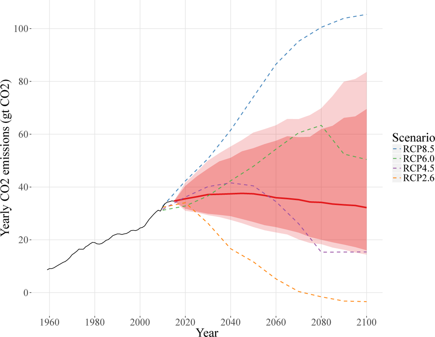
Updated probabilistic forecast of CO2 Emissions, based on data to 2015 and the method of Raftery et al (2017). The forecast median of yearly global emissions in 2100 is now 34 Giga tons.
Figure 2a shows the updated probabilistic forecast of global mean temperature increase from 2015 to 2100 based on current trends. The median forecast for 2100 is 2.8°C, with likely range (90% prediction interval) [2.1, 3.9]°C. The median is 0.4°C lower than that of Raftery et al.1, the upper bound is 1.0°C lower, while the lower bound is 0.1°C higher. The tighter interval reflects the additional five years of data and the improved model.
Figure 2: Probabilistic global temperature forecast and validation.
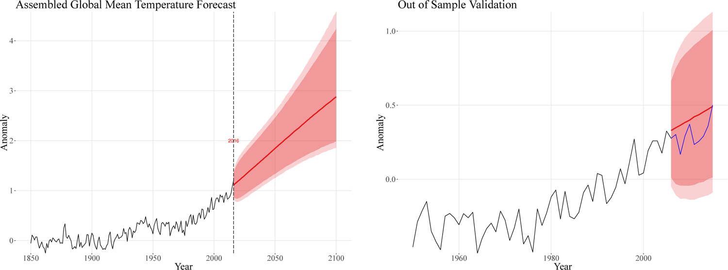
a. Probabilistic forecast of the global temperature anomaly to 2100. The black line represents the historical HadCRUT4 observations, while the red lines and the shaded area represents the forecast median, 90% and 95% prediction interval. Here anomaly stands for the relative difference of global mean temperature to the pre-industrial level, which is taken as the average global mean temperature between 1860–1880. b. Out of sample validation. The black line is the historical anomaly observed from the HadCRUT4 data base for 1960–2005. The red line is the forecasted median, and the dark and light shaded area represent the 50% and 90% predictive intervals for 2006–2015. The blue curve is the observed anomaly in 2006 to 2015. The observations fall well within the predictive distribution.
The previous work showed that the carbon emissions forecasting model validated well in terms of out-of-sample forecasts1. It remains to assess the improved temperature forecasting model. Figure 2b shows the results of a model validation exercise, in which probabilistic forecasts of global temperature were produced for 2006–2015 using data from 1960–2005, and compared with what actually happened. The observations fitted comfortably within the prediction intervals.
Assessment of Paris Agreement
A major component of the Paris Agreement is the NDCs, that were committed to by 185 of the 197 signatory countries5. A further 12 Countries, such as the Philippines, submitted their Intended National Determined Contributions(INDCs), but have not yet formally ratified the Paris Agreement, and so they have not yet submitted NDCs. For these countries, we have taken their NDCs to be the same as their INDCs. We excluded 50 of the 197 countries from our analysis because their promises of cuts in carbon emissions or intensity were unclear. For example, the United Arab Emirates promised to increase the share of “clean energy” in the energy mix to 24% by 2021, but it is unclear how that would actually affect their carbon emissions. For these countries, we assume that they will follow their current trend and we keep the probabilistic forecast of CO2 emissions following the current trend without further emissions reductions.
Of the remaining 147 countries, 81, including 28 combined as the European Union, promised either direct reductions in emissions, such as the USA, or cuts in carbon intensity, such as China. The remaining 66 countries promised emissions cuts relative to the Business As Usual (BAU) scenario; in practice this often means limiting the increase in emissions rather than decreasing them. The BAU scenario assumes essentially that GDP per capita will continue to grow at assumed rates, but that carbon intensity will stay constant. For example, Afghanistan reported its emissions as 28.8 Mt of CO2 equivalent in 2005 and forecast its emissions to be 35.5 and 48.9 Mt in 2020 and 2030 respectively under the BAU scenario. It committed to a reduction of 13.6% relative to BAU for the year 2030, corresponding to 42.7 Mt, an increase of 20% over 2020. Some countries promised a reduction within a specified range, and for these we took the lower bound reduction as their commitment. Most of the NDCs have 2030 as their target date, but some, such as the USA and Brazil, refer to 2025.
For these 147 countries, we translated the NDCs to CO2 emissions using the following steps. For countries such as China that promised reductions in greenhouse gas intensity, rather than in total emissions, we interpret this as promising the same percentage reduction in fossil fuels and industry CO2 intensity. For China, this means reducing emissions by 60% from 2005 to 2030. For countries promising reductions in total greenhouse gas emissions directly, such as the USA, we interpret their NDC as a commitment to the same percentage reduction in CO2 emissions. In the case of the USA, this is a 26% reduction from 2005 levels by 2025.
For countries promising emissions reductions compared to business-as-usual scenarios, we compare the promised emissions levels with the reference year emissions levels (usually total GHG emissions). We then assume that countries are promising the same proportional reduction in fossil fuels and industry CO2 emissions. For example, Vietnam promised an 8% reduction in emissions by 2030, compared to a business-as-usual scenario. According to Vietnam’s NDC11, Vietnam’s total GHG emissions in 2010 were 246.8 million tCO2e, and the projected emissions in 2030 are 787.4 million tCO2e under the BAU scenario. This means that Vietnam promised to limit its emissions in 2030 to no more than 293.5% of the 2010 level. We thus assume that Vietnam promised to limit fossil fuel and industry CO2 emissions to 293.5% of the 2010 level by 2030.
We should point out that most countries have committed to cut total GHG emissions in their NDCs, but here we focus on CO2 emissions and exclude land use emissions. The reason for doing so is two-fold. First, the data for fossil fuels and industry CO2 emissions are more robust and comparable across countries. More importantly, there is a strong relationship between cumulative fossil fuels CO2 emissions and the resulting global mean temperature3. For most climate models, cumulative fossil fuels emissions explain more than 95% of the variance in global mean temperature changes (Table 2). We do not explicitly model non-CO2 forcing agents, but the very high predictive ability of CO2 emissions alone implies that doing so would not greatly change or improve forecasts.
Table 2:
R2 of the linear regression between CMIP 5 model global mean temperature forecast and cumulative fossil fuels and industry CO2 emissions.
| CMIP 5 Models | R2 | slope (°C⋅10−4Gt) |
|---|---|---|
| ACCESS1-0 | 0.99 | 6.3 |
| ACCESS1-3 | 0.98 | 6.2 |
| bcc-csm1-1 | 0.97 | 5.0 |
| bcc-csm1-1-m | 0.92 | 3.6 |
| BNU-ESM | 0.97 | 6.6 |
| … | … | … |
We first address the question, what is the probability that each country will meet its NDC, given current trends? This probability is shown in Figure 3.12 Given current trends, the probabilities are low for most of the major emitters, such as the USA (2%), China (16%) and Japan (10%), Germany (13%) and France (2%). For a few countries, however, such as Russia (93%), they are much higher.
Figure 3: Probability that countries achieve their Paris Agreement Goals according to their nationally determined contributions (NDCs).
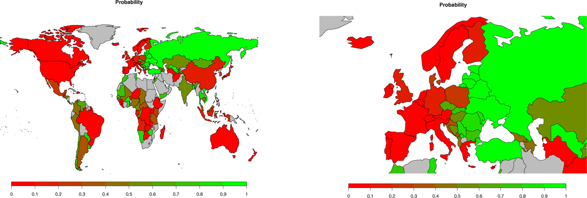
a. All countries. b. European countries. The probabilities vary widely between countries, from values near 0 to values near 1. However, the probabilities are low for most major emitters (USA, China, European Union, Japan).
Next we ask, what is the probability that warming will be kept to 2°C if all countries do meet their NDCs? The NDCs generally refer to 2030, with a few countries referring to 2025, while the Paris Agreement target relates to 2100. Thus the answer to the question depends crucially on what happens after the NDCs are met, i.e. between 2030 (or 2025) and 2100. We consider two scenarios for this. In one scenario, which we call the “Adjusted” scenario, countries revert to their pre-2015 trend after the NDCs are met, in most cases improving their carbon intensity, but at a slower pace than between 2015 and 2030. In the other scenario, which we call the “Continued” scenario, countries continue to improve their carbon intensity at the same rate after they meet the NDC until 2100. Figure 4 shows these emissions scenarios for the top two emitters, USA and China.
Figure 4:
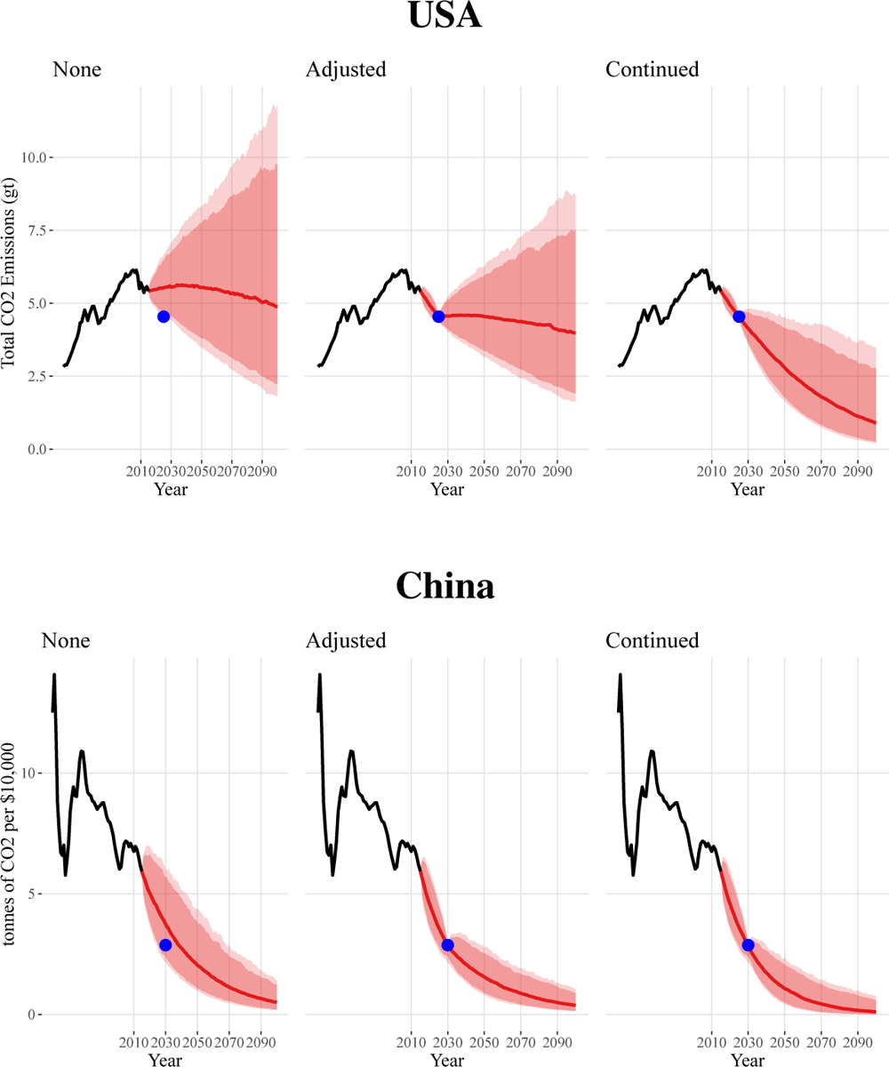
Emissions forecasts for the two largest emitters, under three scenarios: “None” (left), which is the continuation of current trends, “Adjusted” (middle), which assumes that countries will meet their Paris Agreement NDCs, but that these policies will not be continued thereafter, and “Continued” (right), meaning that the policies will continue past the NDC target data (2025 for the USA, 2030 for China). Top: USA. The NDC for the USA is in terms of total emissions, and so the forecast is shown in terms of total emissions. The blue dots represent the NDC target, which is 26% less than yearly emissions in 2005. Bottom: China. The NDC for China is in terms of carbon intensity, and so the forecast of carbon intensity is shown. The blue dots represent the NDC target, which is 60% less than the intensity in 2005. In all the plots, the solid red line is the median forecast, the solid pink shaded area is the likely range, or 90% prediction interval, and the light pink shaded area is the 95% prediction interval.
In 2017, President Trump announced that the USA would withdraw from the Paris Agreement, and it did so in 2020, although President-elect Biden has stated that it will rejoin. Given that US participation in the Paris Agreement remains contested, it remains of interest to assess the consequences of its not participating. We therefore consider a fourth scenario, under which the USA does not meet its NDC and continues emissions in line with current trends, while all other countries make additional efforts and meet their NDCs. The probabilistic forecasts of global mean temperature under all four scenarios are shown in Figure 5.
Figure 5:
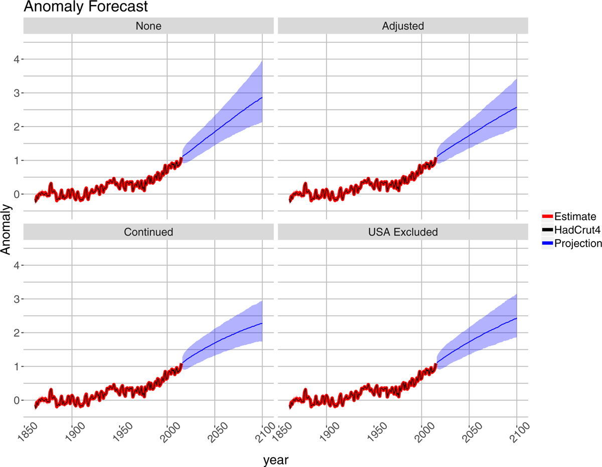
Global Mean Temperature Forecast under different scenarios. The “None”, “Adjusted” and “Continued” scenarios are defined as in Figure 4. The “USA Excluded” scenarios assumes that all countries except the USA meet their NDCs and continue to reduce carbon emissions at the same rate thereafter, while the USA makes no additional effort and emissions follow their current trend. The purple line is the median forecast, while the shaded area is the likely range (90% prediction interval).
We find that on current trends, but without additional efforts to meet the NDCs, the median forecast of global mean temperature increase is 2.8°C, with likely range (90% prediction interval) [2.1, 3.9]°C. If all countries meet their NDCs, but revert to current trends thereafter, the median forecast declines by 0.2°C to 2.6°C, with likely range [2.0, 3.4]°C. If all countries meet their NDCs and continue to reduce carbon emissions at the same rate thereafter, the median forecast declines by a further 0.3°C, to 2.3°C, with likely range [1.8, 2.9]°C. The probability of staying below 2°C is 5% under the “None” scenario, 12% under the “Ajusted” scenario, and 26% under the “Continued” scenario.
If the USA continues on its current trend rather than meeting its NDC, the median forecast of cumulative global carbon emissions would be about 10% (220 Gt CO2) higher than under the “Continued” scenario. The median temperature forecast would then rise to 2.4°C with likely range [1.9, 3.1]°C, and the probability of staying below 2°C would go down from 26% to 18%. Under all the scenarios, the probability of staying below 1.5°C is less than 2%.
Our results suggest that even if all countries meet their promises under the Paris Agreement and continue to reduce emissions at the same rate thereafter, it is unlikely that warming would stay under 2°C, a conclusion also reached by other authors using different approaches13, 14. We therefore ask more precisely, what further reductions would be needed to ensure this? Or, to put it another way, by how much would the emissions reductions promised in the NDCs need to be increased?
Our median forecast of cumulative carbon emissions by 2100 (from 2015) is 3,108 Gt CO2 without the Paris Agreement, and 2,083 Gt CO2 under the “Continued” scenario. We find that to have a 50% chance of limiting warming to 2°C, cumulative emissions would need to be reduced further to 1,579 Gt CO2. Assuming a constant rate of annual decline in global emissions, this would require that the annual rate of decline would need to be 1% to reach the NDCs, and 1.8% to have a 50% chance of staying under 2°C.
While the average rate of decline would need to increase by 80%, this does not mean that the NDCs would need to increase by as much. The needed increase in the NDCs would vary by country, depending on their promises and progress to date. For the largest emitters, the needed increases in the NDCs would be 7% for China, 38% for the USA, 55% for India, 49% for Japan, and 25% for Germany; see Table 1 for more detail. This implies that China needs to increase its 60% carbon intensity cut target to 64%, while the USA needs to increase its 26% emissions cut target to 36%.
Table 1:
Percent increase in emissions reductions relative to the NDCs needed to achieve different objectives in the Paris Agreement for top emitting countries. Russia is not included since currently its emissions are lower than the promises in its NDC. “Even 2°C” refers to a 50% probability of staying below 2°C, and similarly for “Even 1.5°C”, while “Likely 2°C” refers to a 95% probability of staying below 2°C.
| Even 2°C | Likely 2°C | Even 1.5°C | Country |
|---|---|---|---|
| 38% | 125% | 203% | United States |
| 49% | 151% | 229% | Japan |
| 25% | 79% | 120% | Germany |
| 57% | 160% | 215% | Canada |
| 136% | 487% | 875% | South Korea |
| 90% | 165% | 170% | Brazil |
| 17% | 58% | 97% | The United Kingdom |
| 7% | 24% | 41% | China |
| 55% | 147% | 191% | India |
Note that to have an even chance of limiting global warming to 2°C would require global progress towards net zero fossil fuels and industry emissions, but it would not require global annual emissions to reach net zero before 2100, although it would likely involve individual countries doing so. Under this scenario, emissions would need to decline by about 80% relative to their median forecast in the absence of additional efforts (which is roughly equal to the current level), giving global annual emissions of about 7.8 Gt CO2 by 2100.
Similar calculations indicate that to make it likely (90% probability) to stay below 2°C of warming by 2100, rather than just an even chance, would require more than quadrupling the annual rate of decline in emissions. This would require reaching close to global net zero emissions (10% of the current level) by 2070. Many individual countries would need to reach net zero CO2 emissions earlier to achieve this goal.
To have an even chance of staying below 1.5°C would require multiplying the annual rate of decline by about 8, reaching close to global net zero emissions by 2045. To make it likely (90% probability) to stay below 1.5°C would require multiplying the annual rate of decline by almost 30, and reaching close to global net zero by 2023. It is not too surprising that staying below 1.5°C would be so difficult, given that there is already estimated committed warming of 1.1°C15–18.
The 2018 IPCC report on mitigation pathways compatible with staying below 1.5°C has also addressed the question of how this can be done19. They used the same general framework as the IPCC 2014 AR5 report3, basing results on scenarios for future socioeconomic and energy intensity outcomes, combined with ensembles of climate models to translate these into climate outcomes, rather than the fully statistical probabilistic framework we use here. Nevertheless, our results are broadly in line with theirs, albeit with some differences.
They conclude, as do we, that even if the NDCs are met and mitigation continues after 2030, global warming is likely to surpass 1.5°C. They argue that to stay below 2°C in 2100 with probability 66% would require that total GHG emissions decline by 25% from 2010 to 2030, while our method suggests that a reduction of 31% in fossil fuels and industry CO2 would be required to achieve the same goal with probability 50%. The interpretations of probability are different, as theirs are based on ensembles of scenarios and our method produces calibrated probability distributions, but the results are similar. They also conclude that to achieve this would require net zero emissions by 2070. Our method suggests that it would require a 66% reduction in emissions from 2010 to 2070, and that this goal could be achieved without reaching net zero globally. This would, however, require sustained emissions reduction throughout the century, and would require close to net zero emissions to be reached in many countries to achieve the large global total emissions reductions needed.
They conclude that to stay below 1.5°C would require a 45% reduction in emissions from 2010 to 2030, reaching net zero emissions globally by 2050. Our method suggests that this would require an even larger reduction of around 80%, reaching close to net zero emissions by 2045. Again, the results are qualitatively similar.
Discussion
Limitations
Our analysis is based on the data from the Global Carbon Budget20, and so it focuses on forecasting CO2 emissions from fossil fuels and cement production, and the implied global mean temperature. Thus non-CO2 greenhouse gases, such as methane and nitrous oxide, are not explicitly included in the analysis. However, anthropogenic emissions are dominated by CO2, and from our analysis of the current climate models in equation (5), we found that the cumulative fossil fuel and industry emissions from 2015 are linearly related to temperature changes with R2 over 0.95 for most CMIP 5 models. Thus omitting non-CO2 forcing as well as land use CO2 would not change the forecast substantially. It is possible for a specific country to mitigate fossil fuel emissions with high use of biomass energy, which can increase CO2 emissions from the land sector. However, it is unlikely that many major emittors will apply the same type of technologies in the future.
A possible limitation of our model is that we do not forecast negative emissions. Technically, this is because the model is on the logarithmic scale, which yields a model that fits the data well. This does not pose a problem in terms of fitting past data or most plausible future prospects. However, a possible way to achieve the most ambitious goals, such as staying below 1.5°C, would be to compensate for the use of fossil fuels by carbon removal techniques, such as restoring forests or through direct air capture and storage technologies. The possibility of these techniques is considered in scenarios that limit warming to 1.5°C with high overshoot19. One could argue for including them in the model if in the future, direct air capture and storage technologies could be massively adopted, but current technologies are not showing strong evidence that we could rely on them for emissions control. It has been estimated that the Annex I countries could claim a net carbon offset as high as 0.2 GtC per year in this way21. This amount is small relative to the forecast yearly emissions, and we could not find other evidence of a likely large effect of forestation, other than in a few regions, such as some areas of China22. Indeed, in the Amazon rainforest, deforestation does not appear even to be decelerating23–26.
Another limitation of this study is that it addresses the question of how much emissions reduction would be needed to limit global warming to 2 or 1.5°C with given probabilities, but it does not consider how such emissions are to be achieved. This is beyond the scope of the present article, but it has been extensively discussed elsewhere27, 28. We also did not address the issue of equity or fairness in the distribution of emissions reductions among countries, instead assuming that countries’ future efforts would be proportional to their promises under the Paris Agreement. These important questions are beyond our present scope.
In general when we have had to make assumptions not clearly dictated by the data, we have tried to err, if at all, in the direction of tending to favor lower rather than higher emissions, and hence lower temperature increases. For example, while our forecasts of GDP have performed well in out-of-sample validation assessments1, some other probabilistic forecasts of global long-term economic growth are higher29, 30.
Note that our calculations refer to global mean temperature only; the same global mean temperature can yield different spatial temperature distributions31. Also, we have assumed that changes in emissions will be at a roughly constant rate, while in fact of course, the rate of change could change substantially over time32, 33. However, the historical data on which our model is built do indicate that changes in carbon intensity have tended to be incremental and relatively steady over time.
Lastly, there were some data issues. For example, it has been argued that China’s historical emissions have been about 10% lower than assumed here due to different estimates of emissions factors34, but we chose to use the estimate from the Global Carbon Budget, to keep all forecasts comparable.
Other approaches
The present approach is probabilistic, in contrast with the main framework described in the IPCC AR 5 report3, which used four main deterministic scenarios for emissions, called Representative Concentration Pathways (RCPs). There are problems interpreting the RCPs, and from the early days of the IPCC, senior members such as Moss and Schneider called for a statistical forecasting approach such as the one we have used here, in preference to scenarios35. One reason for using deterministic scenarios may have been that official population forecasts, an important input to the emissions forecasts, were then available only as deterministic scenarios. In 2015, however, the UN made its official population projections for all countries probabilistic for the first time2, 36, making it possible to produce probabilistic emissions forecasts soon thereafter1. These are tighter than the full range of the RCPs, but consistent with the two middle RCPs.
There are other proposed methods for probabilistic forecasting of emissions. A different probabilistic approach was taken by Dong et al.37, who used a neural network method to forecast emissions from the top ten emitting countries. Liobikienė and Butkus38 used a statistical approach to forecast emissions for the European Union. These methods focus on subsets of the countries, and so are not comprehensive enough for global emissions forecasts and hence temperature change forecasts.
Overall, unlike most other approaches, our method provides fully statistically-based probabilistic forecasts of the main drivers of future global carbon emissions, and hence of emissions themselves and of the resulting global temperature change, taking account of the associated uncertainty. It is based on a relatively simple Bayesian model, and yet has been found to be well calibrated in out of sample predictive validation experiments, so both the central forecasts and the assessment of uncertainty are satisfactory. This enables us to give statistcally principled assessments of whether countries are on track to meet their NDCs under the Paris agreement, the extent to which the promised reductions are enough to achieve the Paris agreement objectives, and the additional efforts required, complete with the associated uncertainty.
Methods
Data.
We used annual data on population, GDP and carbon emissions for each year from 1960 to 2015 for 161 countries containing over 99% of the world’s population. For population, we used the UN’s 2019 estimates of population for all countries from 1950 to 20159. We produced probabilistic projections for all countries with the model used by the UN for its probabilistic projections36.
GDP per capita data came from the Maddison Project, 2018 version39, using data from 1960 to 2015. This uses purchasing power parity (PPP) rather than market exchange rates, and provides two sets of GDP data, cgdppc for real GDP per capita in 2011US$ with multiple benchmarks, and rgdpnapc for real GDP per capita in 2011US$ with a 2011 benchmark. According to the documentation, rgdpnapc is suitable for cross-country growth comparisons, while cgdppc is more suitable for cross-country income comparisons. Since we are trying to forecast GDP per capita, we use rgdpnapc for GDP.
CO2 emissions data came from the Global Carbon Budget20. We used data from 1960 – 2015.
For historical temperature measures, we used the HadCRUT4 database40, a gridded dataset of historical surface temperature anomalies relative to a 1961–1990 reference period, used by the IPCC3. Data are available for January 1850 onwards and are updated monthly.
We based our forecast on the CMIP 5 model data41. Each experiment on CMIP 5 models includes historical simulations back to 1860, and also provides estimates of future climate changes, either near-term until 2035 or long-term until 2100 or even 2300, under different scenarios.
Model specification.
We built the model in three steps. First we used the model of Raftery et al.1 for probabilistic forecasting of CO2 emissions. This involves Bayesian hierarchical models for fertility and mortality, and hence population, for GDP, and for carbon intensity for each country. We then built Bayesian time series models of CMIP 5 models forecasts and historical simulations, together with the actual historical temperature anomalies, in order to estimate the bias and measurement error variance of the CMIP 5 models. Finally we took the probabilistic forecast of CO2 emissions from the first step as input, and linked the cumulative emissions to the CMIP 5 model forecasts.
The Coupled Model Intercomparison Project Phase 5 (CMIP 5)8, is a standard experimental protocol for studying the output of coupled ocean-atmosphere general circulation models (GCMs). GCMs take inputs such as future forcings, land use, and make corresponding forecasts of global climate. CMIP 5 models take inputs with the RCPs, converting them into radiative forcings and other climate factors, and make forecasts correspondingly. The data are illustrated in Figure 6.
Figure 6:
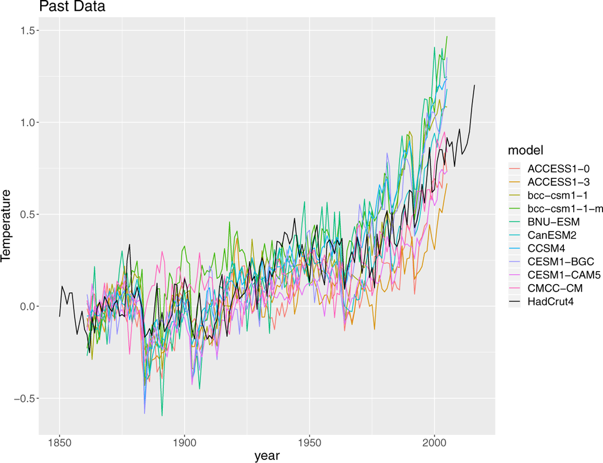
CMIP 5 models. Both model simulations and the observed data are adjusted such that the mean anomaly between 1861–1880 for each model and the observed data is 0. The black line represents the observed data, while the colored lines are for the CMIP 5 model simulations. In total there are 39 CMIP 5 models, but we include only 10 models in this plot for visual clarity.
In this paper, we use our forecasting emissions trajectories as inputs to the GCMs. Instead of running each GCM for each input trajectory of emissions forecasts for probabilistic forecasts, which would not be feasible, we used the existing forecasts with different scenarios of emissions forecasts and developed statistical models of the relationship between CO2 emissions and model forecasts in CMIP 5 models. We found that the forecasts of each CMIP 5 model match linearly with the cumulative emissions for different RCP scenarios, with different correlation and scale. We took our CO2 emissions forecast as input, and used the linear relationship between global mean temperature and the cumulative emissions to generate probabilistic forecasts of future global mean temperature anomalies.
We generated forecasts based on each CMIP 5 model, and then combined these forecasts as an ensemble. For each model, our forecast is based on two parts. The first part takes CO2 emissions trajectories as input, and uses the linear relationship between cumulative CO2 emissions and global mean temperature predictions to generate the CMIP 5 model temperature forecast. The second part takes the uncertainty and bias of the CMIP 5 model forecast directly, based on the difference between historical simulations and the historical temperature anomalies.
For each CMIP 5 model, the historical simulations are generated similarly under different scenarios. We denote the historical simulation of the global mean temperature anomaly in year t from CMIP 5 model i by xi,t. We take the HadCRUT 4 observed temperature anomalies as the observations of the global surface-mean temperature, and denote them by . Then we denote the difference between the CMIP model backcast and the observed value by . We denote the true temperature anomalies by . Then is the difference between the unobserved true global surface-mean temperature anomaly and the backcasts from the CMIP models. Analysis of the autocorrelation and partial autocorrelation functions of the estimated zi,t time series shows that it is well represented by a first-order autoregressive, or AR(1) model. This leads us to specify the following model:
| (1) |
| (2) |
where
| (3) |
| (4) |
where is the variance of the measurement error of HadCRUT 4 observations, and is provided in the HadCRUT 4 dataset.
The forecast anomalies are modeled as linearly related to the cumulative emissions. Therefore, we collected the input cumulative CO2 emissions, denoted by cj,t for scenario or RCP j and year t, and the forecast anomalies from each model xi,j,t, where i indexes models, j indexes scenarios and t indexes years. Then we model the historical simulations as:
| (5) |
This relationship is close to being perfectly linear, as can be seen from the simple linear regression results in Table 2.
Model estimation.
The estimation process for the temperature model has three parts: estimating the model for CO2 emissions, estimating the dynamic model for the bias and measurement error of the CMIP 5 models given by equations (1) and (2), and estimating the model of the connection between CO2 emissions and CMIP 5 model forecasts given by equation (5).
For the model of CO2 emissions, including the population forecasts and the joint model of GDP per capita and carbon intensity, we fitted our model using Markov Chain Monte Carlo (MCMC) sampling, as implemented in the JAGS package in the R programming language. Five chains were used and each chain was run for 100,000 iterations after 5,000 burn-in iterations, and the samples were thinned by 20. Trace plots and standard diagnostics indicated that the number of iterations was big enough.
For the dynamic model for the bias and measurement error of the CMIP 5 models (1, 2), we also fitted our model with MCMC sampling, again implemented in the JAGS R package. For this part, 3 chains were used and each chain was run for 10,000 iterations after 1,000 burn-in iterations. The results are illustrated in Figure 7. Lastly, the models of the connection between emissions and CMIP 5 forecasts were estimated by linear regression.
Figure 7:
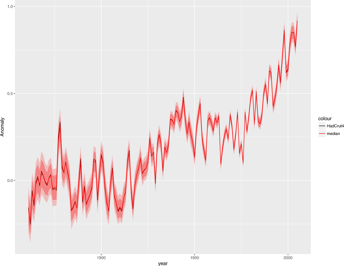
Estimation of historical anomalies. The black line represents the HadCrut4 observations, while the red line and the shaded areas represents the estimated median and the 90% and 95% estimation intervals.
Global mean temperature forecasting.
First we produced probabilistic forecasts of the CO2 emissions for all countries and regions, by making forecasts of population for all countries and forecasts of GDP per capita and carbon intensity jointly. We then drew samples of future population, and sampled jointly from the posterior predictive distribution of GDP per capita and intensity for all future years and countries. We then multiplied them together to obtain posterior trajectories of CO2 emissions. This was repeated 1,000 times to obtain 1,000 posterior samples of future CO2 emissions for all countries and time periods.
We then made forecasts of the CMIP 5 models based on our forecasted CO2 emissions. For each trajectory, we calculated the global cumulative emissions from 2010, denoted by ct. Then, for each CMIP 5 model, the model forecast of global mean temperature xi,t is calculated as bict, where bi is estimated from the linear regression model of equation (5).
We then forecasted the bias and uncertainty of the historical CMIP 5 estimates using equations (1) and (2). For each model i, we drew 1,000 trajectories from the posterior predictive distribution of zi,t up to the year 2100. Finally, we added the xi,t and zi,t forecasts for each trajectory and each CMIP model. We repeated these steps 1,000 times to obtain 1,000 posterior samples of the global mean temperature for each year up to 2100.
The last step is to combine the forecasts from all the CMIP 5 models. We assigned equal weights to the 39 CMIP 5 models. We sampled uniformly from the CMIP models to obtain model i, and given the sampled model i, we sampled one trajectory of xi,t + zi,t from the 1,000 posterior samples. We repeated these steps 1,000 times to obtain the final forecast distribution of the temperature anomalies, shown in Figure 2a.
Temperature forecasting given that countries meet their NDCs
We start from the probabilistic forecasts of the CO2 emissions for all countries and regions given the current trend, with the same procedure as in the previous section. We also summarized the NDCs and INDCs submitted to the Paris Agreement and calculated the target year emissions or intensity. Then for each trajectory and each country, if the forecasted emissions or intensity is higher than their promises, we set an additional decline rate on intensity to move that trajectory, so that it matches with their promises.
Specifically, for countries promising cuts in emissions intensity such as China and India, suppose the promised intensity is JT in year 2015+T, and the forecasted intensity for that trajectory is IT (> JT). Then we need an extra annual intensity cut of from 2016 to the target year. This leads to an expected annual change in the GDP per capita gap by a factor of , where ρ is the correlation between carbon intensity and GDP per capita.
For countries promising emissions cuts directly, such as European countries, suppose the promised emissions are FT in year 2015 + T, and the forecasted intensity for that trajectory is ET. We denote the required extra intensity cut by a per year. Then at the target year 2015 + T, the intensity will be multiplied by a factor of (1 − a)T , while the frontier gap of GDP per capita will be multiplied by a factor of . Since our goal is to increase the emissions cuts in line with commitments or targets, we get the required intensity cut a by solving equation (6) as follows:
| (6) |
For years from 2015 + T to 2100, we forecast each country’s intensity and GDP per capita under different scenarios. Under the “Adjusted” scenario, the intensity and emissions forecast for each trajectory between 2015 + T and 2100 is multiplied by the ratio of promised and forecasted intensity and GDP per capita at the target year 2015+T. Under the “Continued” scenario, for each year 2015 + t from 2015 + T to 2100, assuming the extra annual intensity cut is a factor a, then the intensity forecast is multiplied by the factor of (1 − a)t, and the forecast frontier gap of GDP per capita is multiplied by the factor .
Lastly, we reconstruct the CO2 emissions forecast for all countries and regions, and follow the same procedure with the modified CO2 emissions forecast for global mean temperature forecast for different scenarios.
Required increases in the NDCs to meet the 2°C and 1.5°C warming targets.
To meet the targets requires decreases in cumulative emissions to 2100, but the NDCs are expressed in terms of decreases in annual emissions. We now describe a method for calculating the increases in the NDCs needed to meet the targets, given the required cumulative emissions to 2100.
In the absence of additional efforts, the median forecast turns out to be for total global annual emissions to remain roughly constant from 2016 to 2100, at around A = 3108/85 = 36.6 Gt CO2 per year (see Figure 1). Suppose that to achieve a given climate target with a given probability would require keeping cumulative emissions in 2016–2100 to at most X Gt CO2. Let a be the rate of decline in annual global emissions needed to achieve this, such that if Et is global annual emissions in year 2015 + t, then Et = E0e−at. Then 100 × a is approximately the percent annual decline in global emissions.
To find a, note that cumulative emissions from 2016 to year (2015 + T) from a starting point of 1 Gt CO2 per year in 2016, is
| (7) |
Then a is the solution of the nonlinear equation C(a, T)A = X, and this can be found using a numerical univariate root-finding method.
Let aP be the value of a needed for meeting the Paris Agreement NDCs, assuming that for countries for which the NDCs refer to years before 2030 (such as the USA), the declines in annual emissions continue beyond the NDC target date to 2030 at the same average annual rate. In that case, X = 2083, and solving the equation C(a, T)A = X yields aP = 0.0101, or an average annual rate of decline in emissions of just over 1%.
Each target and probability corresponds to a different value of X, and the corresponding value of a can be calculated in the same way as for the NDCs. For example, to have a 50% chance of staying below 2°C in 2100 requires X = 1579, which corresponds to a = 0.0182, or an average annual rate of decline about 80% higher than needed to meet the Paris NDCs.
We can calculate the corresponding needed increase in NDCs as follows, taking Germany as an example. The NDC for Germany is to reduce carbon emissions by 40% from 1990 to 2030. Germany’s carbon emissions were 1,052 Mt CO2 in 1990, and 795 Mt CO2 in 2015. Thus the NDC for Germany corresponds to a target of 1052 × 0.6 = 630 Mt CO2 in 2030. This requires an annual rate of decline of from 2015 to 2030. To stay below 2°C in 2100 requires a rate of decline that is 0.0182/0.0101 = 1.802 times higher, or 0.0278. This leads to a revised target for 2030 of 795 × (1 − 0.0278)15 = 521. This is a reduction of 50% over the 1990 level, which is 25% more than the NDC level of a 40% reduction. Thus we say that to stay below 2°C in 2100, Germany would need to increase its NDC by 25%.
The calculation is slightly different for countries whose NDCs are expressed in terms of carbon intensity rather than carbon emissions. We assume that GDP is measured in current values in local currency, and we use the numbers reported by the World Bank. We will take China as an example. China’s NDC is to reduce carbon intensity by 60% from 2005 to 2030. China’s carbon emissions in Mt CO2 were 5771 in 2005 and 9717 in 2015. Its GDP was 18.73T yuan in 2005 and 68.60T yuan in 2015. Thus its carbon intensity was 308.1 in 2005 and 141.7 in 2015. We then do the same calculation as we did for Germany, but for carbon intensity instead of carbon emissions. The result is that China’s NDC should become a reduction of 64.2% instead of 60%, an increase of 7% in the promised reduction.
Acknowledgements
This work was supported by NIH grant R01 HD070936. We thank David Battisti, Christopher Bretherton, Jiabin Liu and Hana Ševčíková for comments.
Footnotes
Data Availability. The data and code used to produce the results in this article are available at https://github.com/PPgp/BayesianClimateProjections.
Competing Interests The authors declare no competing interests.
References
- 1.Raftery AE, Zimmer A, Frierson DMW, Startz R & Liu P Less than 2°C warming by 2100 unlikely. Nature Climate Change 7, 637 (2017). [DOI] [PMC free article] [PubMed] [Google Scholar]
- 2.United Nations. World Population Prospects: The 2015 Revision (United Nations, New York, New York, USA, 2015). [Google Scholar]
- 3.Intergovernmental Panel on Climate Change. Climate Change 2013: The Physical Science Basis. Working Group I Contribution to the Fifth Assessment Report of the Intergovernmental Panel on Climate Change (WMO/UNEP, 2014). [Google Scholar]
- 4.UNFCCC. Adoption of the Paris Agreement. http://unfccc.int/resource/docs/2015/cop21/eng/l09r01.pdf (2015). URL http://unfccc.int/resource/docs/2015/cop21/eng/l09r01.pdf.
- 5.United Nations Climate Change. National Determined Contributions. https://www4.unfccc.int/sites/NDCStaging/Pages/Home.aspx (2018). [Online; accessed 19-Sept-2019].
- 6.den Elzen M et al. Are the G20 economies making enough progress to meet their NDC targets? Energy Policy 126, 238–250 (2019). [Google Scholar]
- 7.Roelfsema M et al. Taking stock of national climate policies to evaluate implementation of the Paris agreement. Nature Communications 11, 1–12 (2020). [DOI] [PMC free article] [PubMed] [Google Scholar]
- 8.Hurrell J, Visbeck M & Pirani A WCRP Coupled Model Intercomparison Project–Phase 5, Special Issue of the CLIVAR Exchanges Newsletter (2011).
- 9.United Nations. World Population Prospects: The 2019 Revision (United Nations, New York, New York, USA, 2019). [Google Scholar]
- 10.Lucas RE Some macroeconomics for the 21st century. Journal of Economic Perspectives 14, 159–168 (2000). [Google Scholar]
- 11.Government of Vietnam. Nationally determined contribution of Vietnam (2015).
- 12.South A rworldmap: A new R package for mapping global data. R Journal 3, 35–43 (2011). [Google Scholar]
- 13.Rogelj J et al. Paris Agreement climate proposals need a boost to keep warming well below 2 C. Nature 534, 631–639 (2016). [DOI] [PubMed] [Google Scholar]
- 14.Pan X, den Elzen M, Höhne N, Teng F & Wang L Exploring fair and ambitious mitigation contributions under the Paris Agreement goals. Environmental Science & Policy 74, 49–56 (2017). [Google Scholar]
- 15.Davis SJ, Caldeira K & Matthews HD Future CO2 emissions and climate change from existing energy infrastructure. Science 329, 1330–1333 (2010). [DOI] [PubMed] [Google Scholar]
- 16.Mauritsen T & Pincus R Committed warming inferred from observations. Nature Climate Change (2017). [Google Scholar]
- 17.Brown C, Alexander P, Arneth A, Holman I & Rounsevell M Achievement of Paris climate goals unlikely due to time lags in the land system. Nature Climate Change 9, 203–208 (2019). [Google Scholar]
- 18.Tong D et al. Committed emissions from existing energy infrastructure jeopardize 1.5°C climate target. Nature 572, 373–377 (2019). [DOI] [PMC free article] [PubMed] [Google Scholar]
- 19.Rogelj J et al. Mitigation pathways compatible with 1.5°C in the context of sustainable development. In Masson-Delmotte V et al. (eds.) Global Warming of 1.5°C: An IPCC Special Report on the Impacts of Global Warming of 1.5°C Above Pre-industrial Levels and Related Global Greenhouse Gas Emission Pathways, in the Context of Strengthening the Global Response to the Threat of Climate Change, Sustainable Development, and Efforts to Eradicate Poverty, Chapter 2 (Intergovernmental Panel on Climate Change, 2018). [Google Scholar]
- 20.Le Quéré C et al. Global carbon budget 2018. Earth System Science Data 10, 2141–2194 (2018). [Google Scholar]
- 21.Yamagata Y & Alexandrov GA Would forestation alleviate the burden of emission reduction? An assessment of the future carbon sink from ARD activities. Climate Policy 1, 27–40 (2001). [Google Scholar]
- 22.Huang L, Liu J, Shao Q & Xu X Carbon sequestration by forestation across China: Past, present, and future. Renewable and Sustainable Energy Reviews 16, 1291–1299 (2012). [Google Scholar]
- 23.Shukla J, Nobre C & Sellers P Amazon deforestation and climate change. Science 247, 1322–1325 (1990). [DOI] [PubMed] [Google Scholar]
- 24.Binswanger HP Brazilian policies that encourage deforestation in the amazon. World Development 19, 821–829 (1991). [Google Scholar]
- 25.Boekhout van Solinge T Researching illegal logging and deforestation. Journal of Crime, Criminal Law and Criminal Justice 3, 35–48 (2014). [Google Scholar]
- 26.Fearnside P Business as usual: a resurgence of deforestation in the Brazilian Amazon. Yale Environ 360, 1–6 (2017). [Google Scholar]
- 27.Sustainable Development Solutions Network. Zero Carbon Action Plan (Sustainable Development Solutions Network (SDSN), New York, N.Y., 2020). URL https://www.unsdsn.org/zero-carbon-action-plan. Accessed December 19, 2020. [Google Scholar]
- 28.Larson E et al. Net-Zero America: Potential Pathways, Infrastructure, and Impacts, interim report (Princeton University, Princeton, N.J., 2020). URL https://environmenthalfcentury.princeton.edu. Accessed December 19, 2020. [Google Scholar]
- 29.Müller UK & Watson MW Measuring uncertainty about long-run predictions. Review of Economic Studies 83, 1711–1740 (2016). [Google Scholar]
- 30.Startz R The next hundred years of growth and convergence. Journal of Applied Econometrics 35, 99–113 (2020). [Google Scholar]
- 31.Seneviratne SI et al. The many possible climates from the Paris Agreement’s aim of 1.5°C warming. Nature 558, 41–49 (2018). [DOI] [PubMed] [Google Scholar]
- 32.Rogelj J, Forster PM, Kriegler E, Smith CJ & Séférian R Estimating and tracking the remaining carbon budget for stringent climate targets. Nature 571, 335–342 (2019). [DOI] [PubMed] [Google Scholar]
- 33.Rogelj J et al. A new scenario logic for the Paris Agreement long-term temperature goal. Nature 573, 357–363 (2019). [DOI] [PubMed] [Google Scholar]
- 34.Liu Z et al. Targeted opportunities to address the climate–trade dilemma in China. Nature Climate Change 6, 201–206 (2016). [Google Scholar]
- 35.Moss RH & Schneider SH Towards consistent assessment and reporting of uncertainties in the IPCC TAR: Initial recommendations for discussion by authors. In Pachauri R & Taniguchi T (eds.) Cross-Cutting Issues in the IPCC Third Assessment Report (Cambridge University Press, Cambridge, U.K., 2000). [Google Scholar]
- 36.Raftery AE, Li N, Ševčíková H, Gerland P & Heilig G Bayesian probabilistic population projections for all countries. Proceedings of the National Academy of Sciences 109, 13915–13921 (2012). [DOI] [PMC free article] [PubMed] [Google Scholar]
- 37.Dong C, Dong X, Jiang Q, Dong K & Liu G What is the probability of achieving the carbon dioxide emission targets of the Paris Agreement? Evidence from the top ten emitters. Science of the Total Environment 622, 1294–1303 (2018). [DOI] [PubMed] [Google Scholar]
- 38.Liobikienė G & Butkus M The European Union possibilities to achieve targets of Europe 2020 and Paris agreement climate policy. Renewable Energy 106, 298–309 (2017). [Google Scholar]
- 39.Bolt J, Robert I, de Jong H & van Zanden JL Maddison project database, version 2018. ”rebasing ‘Maddison’: new income comparisons and the shape of long-run economic development”. http://www.ggdc.net/maddison (2018). [Google Scholar]
- 40.Morice CP, Kennedy JJ, Rayner NA & Jones PD Quantifying uncertainties in global and regional temperature change using an ensemble of observational estimates: The HadCRUT4 data set. Journal of Geophysical Research: Atmospheres 117 (2012). [Google Scholar]
- 41.Taylor KE, Stouffer RJ & Meehl GA An overview of CMIP5 and the experiment design. Bulletin of the American Meteorological Society 93, 485–498 (2012). [Google Scholar]