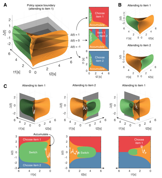
Figure 2. Navigating the optimal policy space.
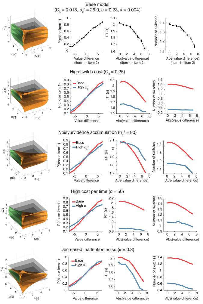
(A) The optimal policy space. The policy space can be divided into regions associated with different optimal actions (choose item 1 or 2, accumulate more evidence, switch attention). The boundaries between these regions can be visualized as contours in this space. The three panels on the right show cross-sections after slicing the space at different values, indicated by the gray slices in the left panel. Note that when (middle panel), the two items have equal value and therefore there is no preference for one item over the other. (B) Optimal policy spaces for different values of (currently attended item). The two policy spaces are mirror-images of each other. (C) Example deliberation process of a single trial demonstrated by a particle that diffuses across the optimal policy space. In this example, the model starts by attending to item 1, then makes two switches in attention before eventually choosing item 1. The bottom row shows the plane in which the particle diffuses. Note that the particle diffuses on the (gray, shaded) plane perpendicular to the time axis of the unattended item, such that it only increases in tj when attending to item j. Also note that the policy space changes according to the item being attended to, as seen in (B). See results text for more detailed description. See Figure 2—figure supplement 1 to view changes in the optimal policy space depending on changes to model parameters.


