Distributional reinforcement learning in the brain

Abstract

Learning about rewards and punishments is critical for survival. Classical studies have demonstrated an impressive correspondence between the firing of dopamine neurons in the mammalian midbrain and the reward prediction errors of reinforcement learning algorithms, which express the difference between actual reward and predicted mean reward. However, it may be advantageous to learn not only the mean but also the complete distribution of potential rewards. Recent advances in machine learning have revealed a biologically plausible set of algorithms for reconstructing this reward distribution from experience. Here, we review the mathematical foundations of these algorithms as well as initial evidence for their neurobiological implementation. We conclude by highlighting outstanding questions regarding the circuit computation and behavioral readout of these distributional codes.

Biological and Artificial Intelligence

The field of artificial intelligence (AI) has recently made rapid progress in algorithms and network architectures that solve complex tasks [1–4]. These advances in AI raise new questions in neurobiology, which ask whether these state-of-the-art algorithms are also used in the brain [5]. Here we discuss a new family of algorithms, termed distributional reinforcement learning (distributional RL; see Glossary) [6,7]. A recent study suggests that the brain’s reward system indeed uses distributional RL [8], opening up opportunities for fruitful interactions between AI and neuroscience.

In this review, we provide an accessible introduction to distributional RL with the hope that it will facilitate such interactions. We first explain the basic algorithms of distributional RL and show that they can be understood from the single, unified perspective of regression. Next, we examine emerging neurobiological evidence supporting the idea that the brain uses distributional RL. Finally, we discuss open questions and future challenges of distributional RL in neurobiology.

Development of Distributional Reinforcement Learning in AI

Reinforcement learning (RL) is the field of AI that studies algorithms by which an agent (e.g. an animal or computer) learns to maximize the cumulative reward it receives [9]. One common approach in RL is to predict a quantity called value, defined as the mean discounted sum of rewards starting from that moment and continuing to the end of the episode [9]. Predicting values can be challenging if the number of states is large and the value function is nonlinear. A recent study overcame these challenges by combining past RL insights with modern artificial neural networks to develop a deep Q-network (DQN) that reached human-level performance in complex video games [2] (Figure 1a–b).

Figure 1. Deep reinforcement learning.

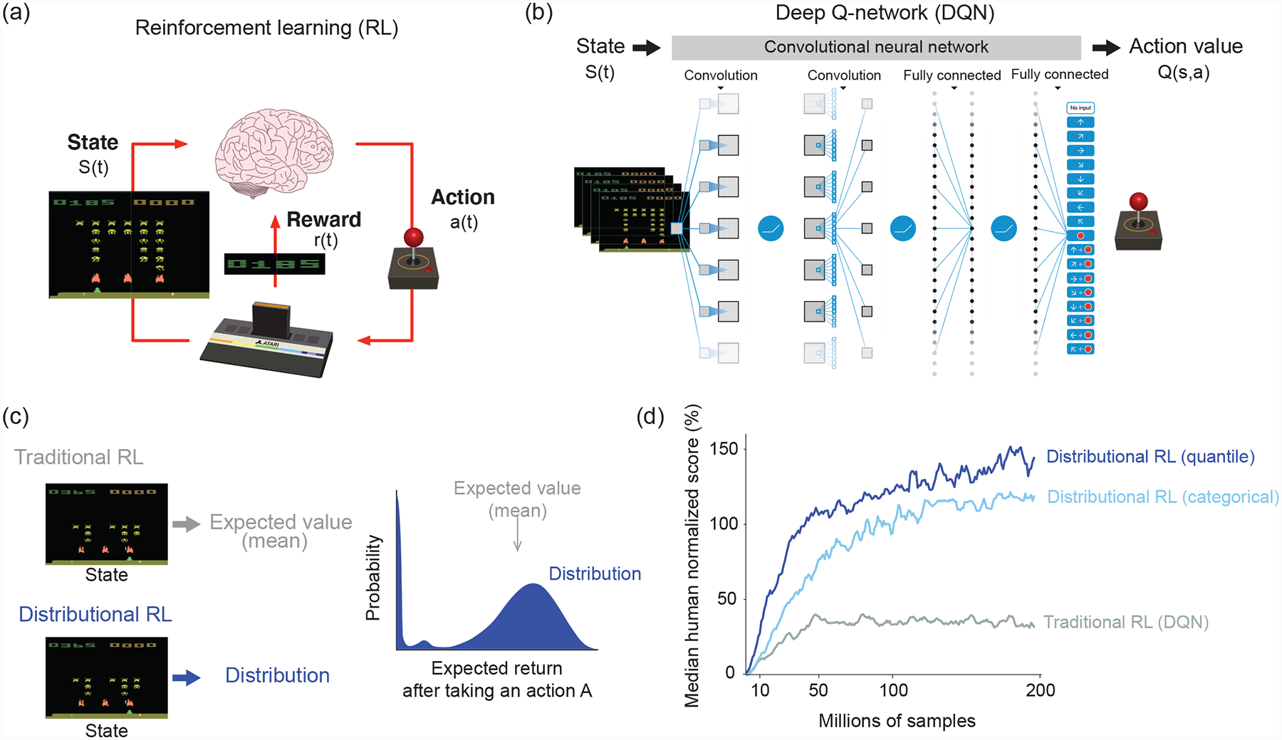
(a) A formulation of reinforcement learning problems. In reinforcement learning, an agent learns what action to take in a given state in order to maximize the cumulative sum of future rewards. In video games such as in an Atari game (here the Space Invader game is shown), an agent chooses which action (a(t), joystick turn, button press) to take based on the current state (s(t), pixel images). The reward (r(t)) is defined as the points that the agent or player earns. After David Silver’s lecture slide (https://www.davidsilver.uk/teaching/).

(b) Structure of deep Q-network (DQN). A deep artificial neural network (more specifically, a convolutional neural network) takes as input a high-dimensional state vector (pixel images of 4 consecutive Atari game frames) along with sparse scalar rewards, and returns as output a vector corresponding to the value of each possible action given that state (called action values or Q-values and denoted Q(s, a)). The agent chooses actions based on these Q-values. To improve performance, the original DQN implemented a technique called “experience replay,” whereby a sequence of events are stored in a memory buffer and replayed randomly during training [2]. This helped remove correlations in the observation sequence, which had previously prevented RL algorithms from being used to train neural networks. Modified after [2].

(c) Difference between traditional and distributional reinforcement learning. Distributional DQN estimates a complete reward distribution for each allowable action. Modified after [6].

(d) Performance of different RL algorithms in DQN. Gray, DQN using a traditional RL algorithm [2]. Light blue, DQN using a categorical distributional RL algorithm (C51 algorithm [6]). Blue, DQN using a distributional RL based on quantile regression [7]. Modified after [7].

Various algorithms have been developed to improve upon DQN [10], including distributional RL [6,7]. The key innovation of distributional RL lies in how these algorithms predict future rewards. In environments where rewards and state transitions are inherently stochastic, traditional RL algorithms learn to predict a single quantity, the mean over all potential rewards. Distributional RL algorithms, by contrast, learn to predict the entire probability distribution over rewards (Figure 1c). Remarkably, modifying DQN to implement variants of distributional RL boosts performance by as much as two and a half times [6,7,10] (Figure 1d).

How Distributional Reinforcement Learning Works

Two major topics in distributional RL are (i) how the reward distribution is represented, and (ii) how it is learned. The original distributional RL algorithm [6] used data structures akin to histograms (the number of samples falling into fixed bins, or categories) to represent a distribution and treated learning as a multiclass classification problem. This class of distributional RL is hence called “categorical” distributional RL [6]. Although using a histogram is an intuitive (and common) way to represent a distribution, it remains unclear whether neurons in the brain can instantiate this approach. A subsequent paper proposed to replace the histogram representation by an algorithm called quantile regression [7], which uses a novel population coding scheme to represent a distribution and a biologically-plausible learning algorithm to update it.

Learning from Prediction Errors

One of the key ideas in RL is that learning is driven by prediction errors, the discrepancy between actual and expected outcomes [11,12]. This idea originated in animal learning theories, and was formulated mathematically by Rescorla and Wagner [13]. The Rescorla-Wagner rule postulates that the strength of association between two stimuli is updated based on a prediction error. In the simplest case, when a stimulus (X) is presented, the animal predicts the value of the future outcome. Once this outcome is revealed, it compares the outcome (R) against the predicted value (V) and computes the prediction error δ≔ R − V. According to the Rescorla-Wagner rule, the value of stimulus X is updated in proportion to the prediction error:

$$V\leftarrow V+\alpha \cdot \delta .$$ (1)

Here, α is the learning rate parameter, which takes a value between 0 and 1. Eq. (1) defines how the value V is updated. (The arrow indicates that V on the left-hand side is the value after updating whereas V on the right-hand side is the value before.) If R is constant, the predicted value gradually approaches the actual value and the prediction error approaches 0. Even if R is probabilistic, the predicted value will converge to the mean reward amount, at which point positive and negative prediction errors will balance across trials (Figure 2a). In a more sophisticated RL algorithm called temporal difference (TD) learning [9,11,12], the prediction error is computed based on the difference between the predicted values at consecutive time points (Box 1), but the update rule may otherwise remain the same.

Figure 2. Learning rules of distributional RL (quantile and expectile regression).

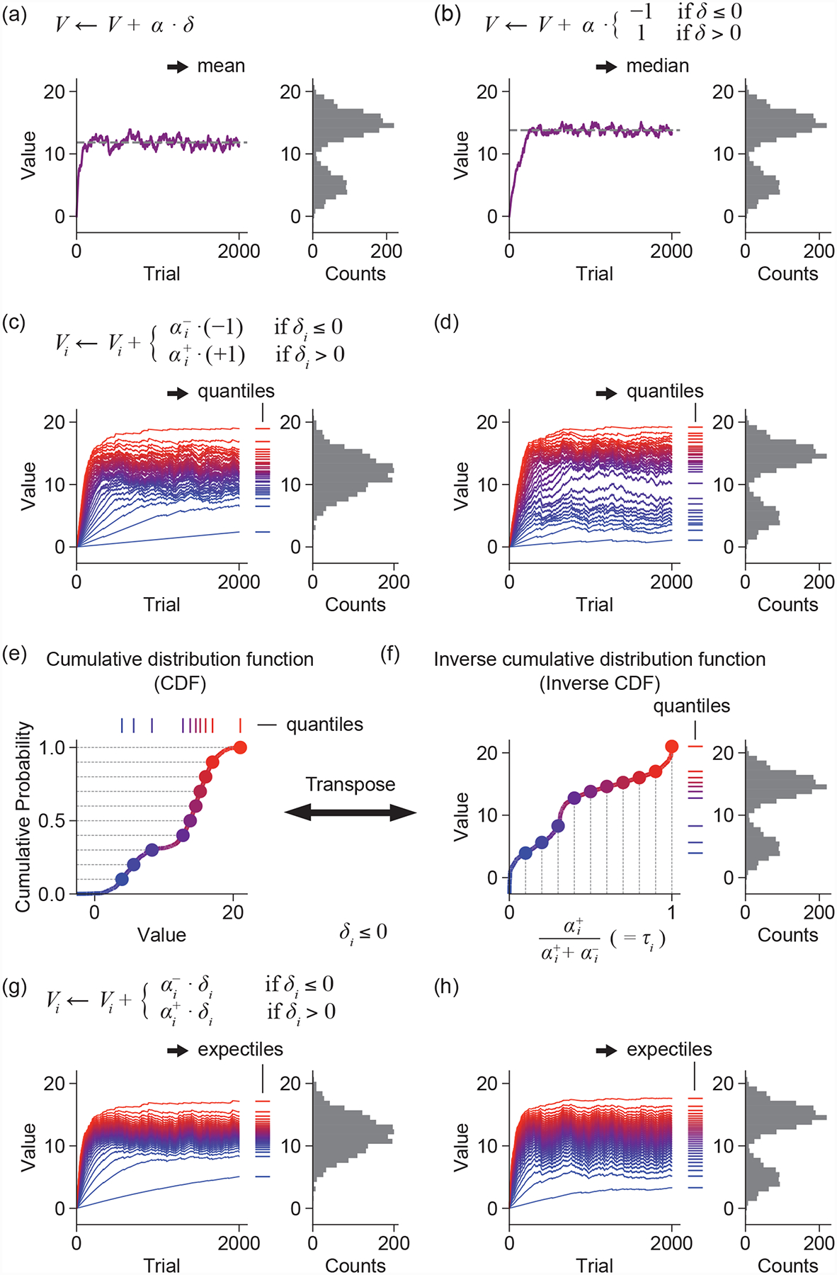
(a) The standard Rescorla-Wagner learning rule converges to the mean of the reward distribution.

(b) Modifying the update rule to use only the sign of the prediction error causes the associated value predictor to converge to the median of the reward distribution.

(c-d) Adding diversity to the learning rates alongside a binarized update rule that follows the sign of the prediction error causes a family of value predictors to converge to quantiles of the reward distribution. More precisely, the value $q_{{\tau }_i}$ to which predictor i converges is the τ_i-th quantile of the distribution, where τ_i is given by $\frac{{\alpha }_i^{+}}{{\alpha }_i^{+}+{\alpha }_i^{-}}$. This is illustrated for both unimodal (c) and bimodal (d) distributions.

(e) The cumulative distribution function (CDF) is a familiar representation of a probability distribution.

(f) By transposing this representation, we get the quantile function, or inverse CDF (left). Uniformly-spaced quantiles cluster in regions of higher probability density (right). Together, these quantiles encode the reward distribution in a non-parametric fashion.

(g-h) Multiplying the prediction error by asymmetric learning rates yields expectiles. Relative to quantiles, expectiles are pulled toward the mean for both unimodal (g) and bimodal (h) distributions.

Box 1. Temporal Difference Learning.

The Rescorla-Wagner (RW) rule [13], for all its success, is limited by its exclusive focus on immediate rewards. Fortunately, many of its shortcomings can be overcome by defining a different environmental structure and learning objective [9,11,12]. We start by considering arbitrary states s, which transition at each time step and sample a random reward (possibly zero or negative) from a probability distribution R(s_t). We then define a new learning objective, the value:

$$V\left(s_t\right):=E\left[R\left(s_t\right)+\gamma R\left(s_{t+1}\right)+{\gamma }^{2}R\left(s_{t+2}\right)+\dots \right],$$ (1.1)

where E[·] denotes an expectation over stochastic state transitions and reward emissions, and γ is a discount factor between 0 and 1, reflecting a preference for earlier rewards.

Contrary to the RW model, which cares only about the reward obtained in a trial, this model cares about (a weighted sum of) all future rewards. Since the environment is assumed to follow Markov dynamics, we can rewrite this relationship recursively, using the so-called Bellman equation:

$$V\left(s_t\right):=E\left[R\left(s_t\right)+\gamma V\left(s_{t+1}\right)\right].$$ (1.2)

Rearranging and sampling r_t ~ R(s_t) from the environment, we arrive at a new kind of reward prediction error, namely, a temporal difference (TD) error [4], which we also call δ to emphasize its similarity to the reward prediction error in the RW model:

$$\delta (t):=r_t+\gamma V\left(s_{t+1}\right)-V\left(s_t\right).$$ (1.3)

The value update then occurs in exactly the same manner as before:

$$V\left(s_t\right)\leftarrow V\left(s_t\right)+\alpha \delta (t).$$ (1.4)

The similarity between the RW and TD learning rules disguises one important difference. In the case of the RW rule, we computed the prediction error using the actual reward, R, that was experienced. In TD, we substitute R with r_t + γV(s_t+1), our estimate of the target value of state s_t. But this target includes yet another value predictor γV(s_t+1), which we also are trying to learn, and which may in fact be inaccurate. Therefore, we use one estimate to refine a different estimate, a procedure known as “bootstrapping.” For that reason, unlike RW, TD learning is not a true instance of stochastic gradient descent, since changing the parameters of our value function changes not only our estimate but also our target [9]. This is the principal reason why we focus on distributional forms of the RW (rather than TD) rule in the main text. Nonetheless, and quite remarkably, this “bootstrapping” procedure is proven to converge to a point near the local optimum in the case of linear function approximation [88], and can be made to work very well in practice even in situations where theoretical convergence is not guaranteed [2].

Toward Distributional RL

While expected values can be useful, summarizing a situation by just a single quantity discards information that may become important in the future. If the demands of the animal change — for example, if large, uncertain rewards become preferred to smaller, certain ones [14] — animals that store more detailed information about outcomes may perform better. Learning entire distributions sounds computationally expensive, but interestingly, distributional RL can arise out of two simple modifications to Eq. (1) [7,8].

First, we “binarize” the update rule as follows,

$$V\leftarrow V+\alpha \cdot \{\begin{array}{cc}-1& \text{ if }\delta \le 0\\ 1& \text{ if }\delta >0\end{array}.$$ (2)

That is, the prediction error (δ) in the update equation is replaced by +1 or −1 depending on the sign of δ, such that value predictions are incremented (or decremented) by a fixed amount. In this case, V will converge to the median rather than the mean of the reward distribution (Figure 2b). Intuitively, this is because the median is the value that divides a distribution such that a sample from the full distribution is equally likely to fall above or below it. The increments and decrements specified by Eq. (2) will balance out at the point where positive and negative prediction errors occur with exactly the same frequency, which is to say, when V is the median of the reward distribution.

The second modification is to add variability in learning rate (α). Suppose we have a family of value predictors, V_i, each of which learns its value prediction in a slightly different way [7,8]. We assign each V_i two separate learning rates, an ${\alpha }_i^{+}$ for positive prediction errors and an ${\alpha }_i^{-}$ for negative prediction errors, resulting in the learning rule

$$V_i\leftarrow V_i+\{\begin{array}{ll}{\alpha }_i^{-}\cdot (-1)\hfill & \text{ if }{\delta }_i\le 0\hfill \\ {\alpha }_i^{+}\cdot (+1)\hfill & \text{ if }{\delta }_i>0\hfill \end{array}.$$ (3)

In the case where ${\alpha }_i^{+}>{\alpha }_i^{-}$, positive prediction errors drive learning more strongly compared to negative ones. This will cause V_i to converge to a value larger than the median, so we call such value predictors “optimistic”. Conversely, when ${\alpha }_i^{+}<{\alpha }_i^{-}$, the value predictors become “pessimistic.” For any combination of ${\alpha }_i^{+}$ and ${\alpha }_i^{-}$, a value predictor which learns according to the above rule will converge to the $\frac{{\alpha }_i^{+}}{{\alpha }_i^{+}+{\alpha }_i^{-}}={\tau }_i\text{-th}$ quantile (Figure 2c–d). Multiple value predictors associated with different τ_i’s thus form a population code that is the inverse of the cumulative distribution function (CDF; Figure 2e–f) of rewards.

We can also consider a family of value predictors that retains the original form of the update rule in Eq. (1), such that

$$V_i\leftarrow V_i+\{\begin{array}{ll}{\alpha }_i^{-}\cdot {\delta }_i\hfill & \text{ if }{\delta }_i\le 0\hfill \\ {\alpha }_i^{+}\cdot {\delta }_i\hfill & \text{ if }{\delta }_i>0\hfill \end{array}.$$ (4)

This update rule gives rise to a range of value estimates called expectiles (Figure 2g–h), which generalize the mean just as quantiles generalize the median. However, unlike quantiles, expectiles do not bear a straightforward relationship to the CDF. To understand them, it is necessary to adopt a more general perspective on learning.

Distributional Reinforcement Learning as the Process of Minimizing Estimation Errors

The distributional RL algorithms illustrated above are known as quantile and expectile regression [7,8]. This is because in addition to thinking of quantiles as places to divide ordered samples into two sets of given size ratios, they can be derived from the perspective of minimizing certain continuous loss functions, which is precisely what a regression does [15,16]. We will demonstrate this here by re-deriving the aforementioned learning algorithms for quantiles and expectiles from the common perspective of regression (Figure 3a).

Figure 3. Distributional RL as minimizing a loss function.

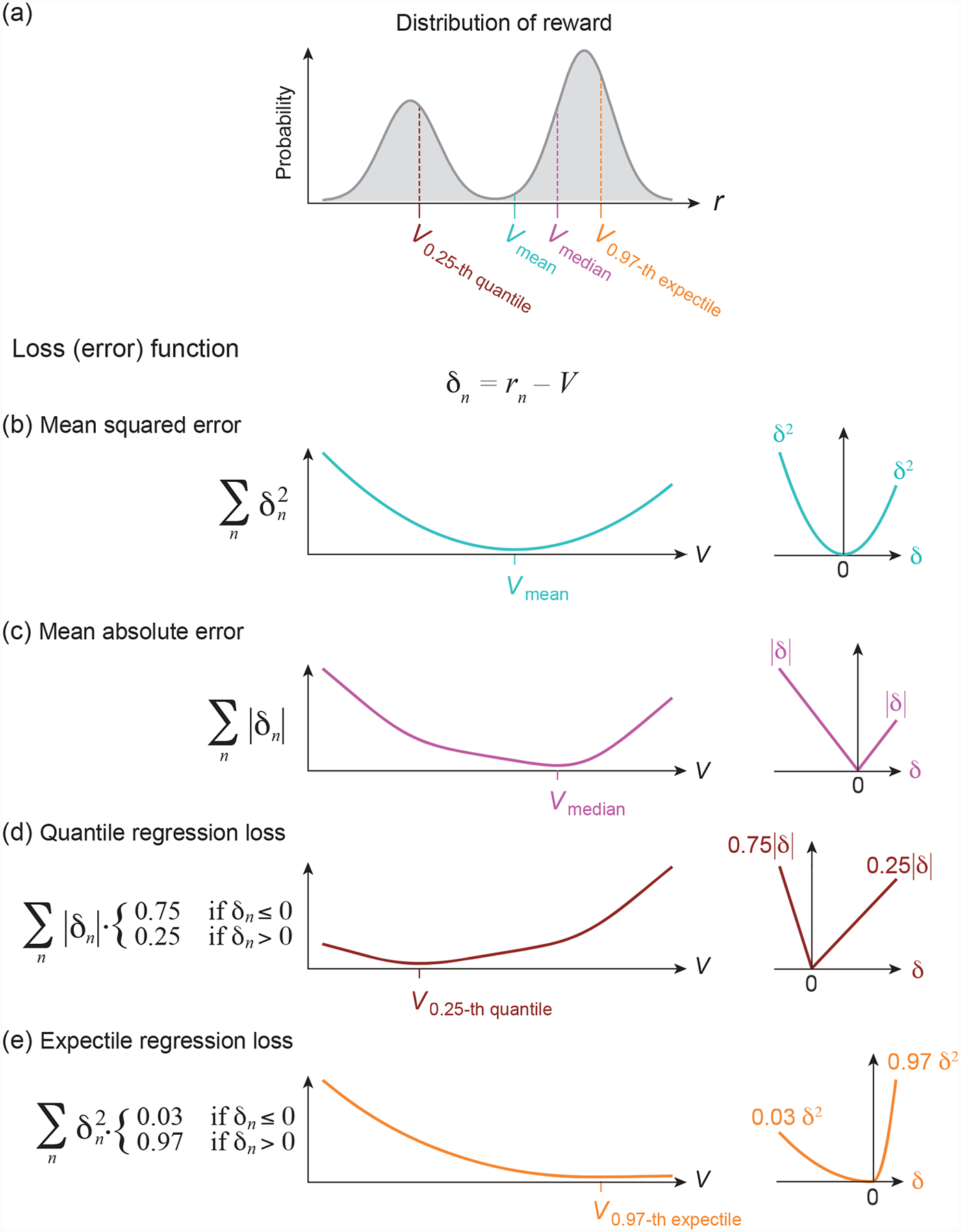
(a) The reward probabilities of an example reward distribution. Mean V_mean, median V_median, 0.25-quantile V_{0.25-quantile} and 0.97-expectile V_{0.97-expectile} of this distribution are indicated with different colors.

(b-e) Loss as a function of the value estimate V (left) when the rewards follow the distribution presented in (a), illustrating that V = V_mean minimizes the mean squared error (b), V = V_median minimizes the mean absolute error (c), V = V_{0.25-quantile} minimizes the quantile regression loss for τ = 0.25 (d), and V = V_{0.97-expectile} minimizes the expectile regression loss for τ = 0.97 (e). The right panels show the loss as a function of the RPE δ.

Let us first consider the most widespread error measure used in linear regression, the mean squared error (MSE), in the context of learning about rewards (r). Assuming that we have observed rewards r₁, r₂, …, r_N across N trials, the MSE of some value V is defined as

$$MSE(V)=\frac{1}{N}{\sum }_{n=1}^N{\left(r_n-V\right)}^2,$$ (5)

and so measures the squared difference of this value to each observed reward, averaged across all rewards [17]. This definition makes the MSE a function of V, such that as the value of V changes, the MSE will increase or decrease (Figure 3b). The question that we want to ask is: what is the V that minimizes the MSE? To find this minimum, we set the derivative of the MSE with respect to V to zero and solve for V, resulting in $V=\frac{1}{N}{\sum }_{n=1}^N{r}_n$. Therefore, if one defines the prediction error associated with the nth reward as δ_n = r_n − V, then the MSE (the mean across all ${\delta }_n^2$) is minimized if V equals the average reward across trials.

One approach to minimize Eq. (5) is to memorize all rewards across trials and subsequently compute their mean. However, once the number of trials N is large, this method is neither memory-efficient nor biologically plausible. An alternative method that is widely applied in machine learning is stochastic gradient descent [18]. Revisiting the above example, assume that the rewards r₁, r₂, …, r_N are observed one after the other. We would like to find a local learning rule that allows us to come up with an estimate V that approximately minimizes the sum of squared prediction errors.

With stochastic gradient descent, the current reward estimate V is adjusted every time a new observation r_n becomes available by moving one small step down along the gradient of the squared error. (For mathematical convenience, here we actually compute the gradient of half the squared error, $\nabla \left({\delta }_n^2/2\right)$, but the conceptual approach is the same.) This gradient measures how the output of the loss function associated with this new observation, ${\delta }_n^2$, will change when the relevant parameters are modified. In this case, the relevant parameter is just V, such that the required gradient is given by the derivative of ${\delta }_n^2/2$ with respect to V:

$$\begin{gathered} \nabla \left({\delta }_n^2/2\right)=\frac{d{\left(r_n-V\right)}^2/2}{dV} \\ =-\left(r_n-V\right) \\ =-{\delta }_n. \end{gathered}$$

The parameter V will then be updated according to $V\leftarrow V-\alpha \nabla \left({\delta }_n^2/2\right)$. After substituting the gradient, we obtain

$$V\leftarrow V+\alpha \cdot {\delta }_n.$$ (6)

The current error function, which depends only on the most recently available reward r_n, here acts as a proxy of the error function encompassing all trials, Eq. (5). Intuitively speaking, subtracting α times the gradient from the current reward estimate, as performed in Eq. (6), corresponds to adjusting the reward estimate slightly towards the steepest drop of the current error function. Notice that Eq. (6) is equivalent to Eq. (1). Therefore, the Rescorla-Wagner rule is equivalent to stochastic gradient descent if we measure the loss by the mean squared error [19].

In general, as long as the error we aim to minimize has a form similar to Eq. (5), in which the global error is a sum of local errors, each of which only depends on the reward in one trial, we can always apply an update rule similar to Eq. (6), using the corresponding gradient to carry out stochastic gradient descent. Below, we apply this approach to a variety of loss functions to derive the corresponding update rules.

One simple change is to replace the square of δ_n by its absolute value, leading to the mean absolute error

$$\frac{1}{N}{\sum }_{n=1}^N\left|{\delta }_n\right|.$$ (7)

In this case, the derivative with respect to V of |δ_n| = |r_n – V| is simply −sign(δ_n), which readers will recognize as the update that converges to the median of the reward distribution (Figure 3c).

If we additionally weigh positive and negative errors differently,

$$\frac{1}{N}{\sum }_{n=1}^N\left|{\delta }_n\right|\cdot \{\begin{array}{cc}1-\tau & \text{ if }{\delta }_n\le 0\\ \tau & \text{ if }{\delta }_n>0\end{array},$$ (8)

where τ is a fixed value between 0 and 1, the best estimate becomes the τ-th quantile of the reward distribution [16]. Hence, Eq. (8) is called the quantile regression loss function.

We can again turn the global error function, Eq. (8), into a sequential update by stochastic gradient descent, resulting in

$$V\leftarrow V+\alpha \cdot \{\begin{array}{cc}-(1-\tau )& \text{ if }{\delta }_n\le 0\\ \tau & \text{ if }{\delta }_n>0\end{array}.$$ (9)

If δ_n is negative, the rate parameter equals −α(1 – τ) = −α⁻; if it is positive, this product becomes ατ = α⁺. This confirms the intuition developed in the preceding section (Eq. 3), showing that such an update rule indeed minimizes the quantile regression loss function and approximates the τ-th quantile (Figure 3d).

To arrive at expectile regression, we move one step further and replace the absolute value of δ_n with its square in Eq. (8). This yields the weighted squared error loss function, also called the expectile regression loss function [15,20],

$$\frac{1}{N}{\sum }_{n=1}^N{\delta }_n^2\cdot \{\begin{array}{cc}1-\tau & \text{ if }{\delta }_n\le 0\\ \tau & \text{ if }{\delta }_n>0\end{array},$$ (10)

whose associated best estimate is the τ-th expectile (Figure 3e). For τ = 0.5, the two weights are equal, such that the error measure becomes equivalent to the mean squared error, Eq. (1). This confirms that the 0.5-th expectile is the mean across all rewards. Other expectiles can be interpreted as the analogue to quantiles, but for squared rather than absolute errors.

Stochastic gradient descent on Eq. (10) results in the update rule

$$V\leftarrow V+\alpha {\delta }_n\cdot \{\begin{array}{cc}1-\tau & \text{ if }{\delta }_n\le 0\\ \tau & \text{ if }{\delta }_n>0\end{array},$$ (11)

which is a modified version of Rescorla-Wagner rule in which the rate parameter takes on different values for negative and positive δ_n (Eq. 4).

Different loss functions therefore lead to estimating different statistics of the reward distribution. Even if we fix a loss function, however, there are still many possible ways to represent and learn the corresponding statistic. For instance, instead of storing the estimated quantiles directly and performing updates on them as in Eq. (9), the brain may approximate quantiles by a parametric vector-valued function q(θ) = (q₁(θ), …, q_M(θ)), with parameters θ that might correspond to synaptic strengths between different neurons and outputs q_i denoting the value of the τ_i-th quantile. The same strategy could also apply to expectiles e(θ).

To find the update rules for these representations, we can again use stochastic gradient descent. However, rather than computing the gradient with respect to V, we now compute it with respect to the function’s parameters, θ. Following similar calculations as shown above, this update rule for learning quantiles turns out to be

$$\theta \leftarrow \theta +\alpha {\sum }_{i=1}^M{\nabla }_{\theta }{q}_i(\theta )\cdot \{\begin{array}{cc}-(1-\tau )& \text{ if }{\delta }_{i,n}\le 0\\ \tau & \text{ if }{\delta }_{i,n}>0\end{array},$$ (12)

while for learning expectiles, it becomes

$$\theta \leftarrow \theta +\alpha {\sum }_{i=1}^M{\delta }_{i,n}{\nabla }_{\theta }{e}_i(\theta )\cdot \{\begin{array}{cc}1-\tau & \text{ if }{\delta }_{i,n}\le 0\\ \tau & \text{ if }{\delta }_{i,n}>0\end{array}.$$ (13)

Thus, the only changes to the update rules are (i) the addition of the gradient terms ∇_θq_i(θ) or ∇_θe_i(θ), and (ii) the sum of contributions from different component quantiles or expectiles. For components q_i(θ) or e_i(θ) estimated as linear parametric functions $u_i^T\theta +v_i$, this gradient is u_i, which results in a simple re-scaling of the parameter update by u_i. Such functions include single-layer neural networks, in which case it is synaptic weights that are incremented or decremented. If we move from linear to non-linear parametric functions, like multi-layer neural networks, the gradients (and therefore the updates) become slightly more complex, but the general principles of stochastic gradient descent remain.

Traditional and Distributional Reinforcement Learning in the Brain

The idea that the brain uses some form of RL to select appropriate actions has been supported by a number of observations of animal behavior and neuronal activity [12,13,21–23]. One of the strongest pieces of evidence is the close relationship between the activity of dopamine neurons and the reward prediction error (RPE) term in RL algorithms [21–23]. Neural activity representing value, the other critical variable in these algorithms, is also found in dopamine-recipient areas [24–26].

Dopamine neurons are located mainly in the ventral tegmental area (VTA) and substantia nigra pars compacta (SNc) in the midbrain, from which they send long axons to a wide swath of the brain that includes striatum, prefrontal cortex and amygdala. The information conveyed by different dopamine neurons varies greatly based on their projection targets [27–30], with the dopamine neurons in the VTA that project to the ventral part of the striatum (nucleus accumbens) thought to mainly signal RPEs (but see [31,32]). Beyond this coarse projection specificity, which has been reviewed elsewhere [27,28], there is also fine-grained diversity within VTA dopamine neurons, which is our focus here. While the activity of these neurons appears quite homogenous compared to neurons in other parts of the brain [33,34], recent studies have revealed more diverse firing patterns [35] at least some of which may reflect systematic variation in RPE signals [36]. Distributional RL offers one possible explanation for the functional significance of this diversity within the VTA.

Testing Distributional Reinforcement Learning

The key ingredient that transforms traditional RL into distributional RL is the diversity in learning rate parameters for positive and negative RPEs (α⁺and α⁻), or, more critically, the ratio between them, $\tau =\frac{{\alpha }^{+}}{{\alpha }^{+}+{\alpha }^{-}}$, which we call the asymmetric scaling factor [7,8]. Although the biological processes that implement α⁺ and α⁻ remain unclear, one possibility is that these parameters correspond to how the firing of each dopamine neuron scales up or down with respect to positive or negative RPEs, respectively. This leads to several testable predictions in the expectile setting.

First, there should be ample diversity in asymmetric scaling factors across dopamine neurons (Figure 4a), which should result in optimistic and pessimistic value predictors (Figure 4b). The information contained in these value predictors (V_i), in turn, is routed back to dopamine neurons for computing RPEs, subtracting “expectation” (V_i) from the response to a received reward (R). This means that for optimistic dopamine neurons, which are coupled to relatively high value predictors, larger rewards are necessary to cancel out their reward response and obtain zero RPE. Thus, optimistic dopamine neurons with α⁺ > α⁻ will have “reversal points” that are shifted towards above-average reward magnitudes (Figure 4c). Conversely, pessimistic dopamine neurons with α⁺ < α⁻ will have reversal points shifted towards below-average reward magnitudes. Across the population of neurons, distributional RL therefore makes the unique prediction that the reversal points of dopamine response functions should be positively correlated with their asymmetric scaling factors ($\tau =\frac{{\alpha }^{+}}{{\alpha }^{+}+{\alpha }^{-}}$).

Figure 4. The structured diversity of midbrain dopamine neurons is consistent with distributional RL.

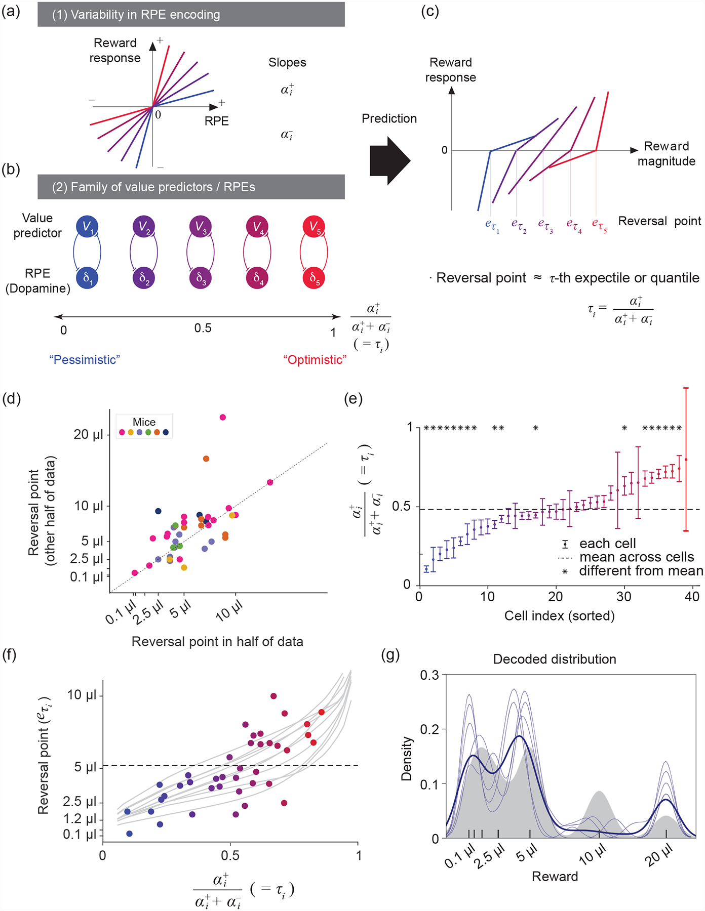
(a) Schematic of five different response functions (spiking activity of dopamine neurons) to positive and negative RPEs. In this model, the slope of the response function to positive and negative RPEs corresponds to the learning rates α⁺ and α⁻. Diversity in α⁺ and α⁻ values results in different asymmetric scaling factors ($\frac{{\alpha }_i^{+}}{{\alpha }_i^{+}+{\alpha }_i^{-}}$).

(b) RPE channels (δ_i) with α⁺ < α⁻ overweight negative prediction errors, resulting in pessimistic (blue) value predictors (V_i), while RPE channels with α⁺ > α⁻ overweight positive prediction errors and result in optimistic (red) value predictors. This representation corresponds to the Rescorla-Wagner approach in which RPE and value pairs form separate channels, with no crosstalk between channels with different scaling factors. See Box 2 for the general update rule when this condition is not met.

(c) Given that different value predictors encode different reward magnitudes, the corresponding RPE channels will have diverse reversal points (reward magnitudes that elicit no RPE activity relative to baseline). The reversal points correspond to the values V_i of the τ_i-th expectiles of the reward distribution.

(d) Reversal points are consistent across two different halves of the data, suggesting that the diversity observed is reliable (P = 1.8 × 10⁻⁵, each point represents a cell). Modified after [8].

(e) Diversity in asymmetric scaling in dopamine neurons tiles the entire [0, 1] interval and is statistically reliable (one-way ANOVA; F(38,234) = 2.93, P = 4 × 10⁻⁷). Modified after [8].

(f) Significant correlation between reversal points and asymmetric scaling in dopamine neurons (each point is a cell, linear regression P = 8.1 × 10⁻⁵). Grey traces show variability over simulations of the distributional TD algorithm run to calculate reversal points in this task. Modified after [8].

(g) Decoding of the reward distribution from dopamine cell activity using an expectile code. The expectiles of the distribution, $\left\{{\tau }_i,e_{{\tau }_i}\right\}$, were defined by the asymmetries and reversal points of dopamine neurons. Grey area represents the smoothed reward distribution, light blue traces represent several decoding runs, and the dark blue trace their mean. Modified after [8].

A recent study [8] tested these predictions using existing data from optogenetically-tagged VTA dopamine neurons in mice performing a task in which a single odor preceded a variable reward [34,37]. Responses differed in subtle but important ways among dopamine neurons; some neurons were consistently excited, even for below-average rewards, while others were excited only by rewards that exceeded the average (Figure 4d) [8]. The reversal points in this task were assumed to reflect different value predictions: each reversal point $e_{{\tau }_i}$ was interpreted as the τ_i-th expectile of the reward distribution.

To independently compute τ_i, ${\alpha }_i^{+}$ and ${\alpha }_i^{-}$ were estimated for each neuron i as the slopes of the average response function above and below the neuron’s reversal point. This analysis revealed significant variability in asymmetric scaling factors, tiling a relatively wide range between 0 and 1 (Figure 4e). Critically, these asymmetric scaling factors were positively correlated with the reversal points, as predicted above (Figure 4f). Finally, such structured heterogeneity in dopamine neurons allowed the authors to decode possible reward distributions from the neural data by finding reward distributions compatible with the expectiles defined by $\left\{{\tau }_i,e_{{\tau }_i}\right\}$ (Figure 4g). Importantly, this decoding procedure strongly relied on the structured heterogeneity assumption imposed by an expectile code and should have been unsuccessful if the variability merely reflected random noise.

Distributional RL lends itself to several additional experimental predictions, which remain to be tested [8]. For example, dopamine neurons should show consistent asymmetric scaling factors across different reward distributions. Furthermore, optimistic cells should learn more slowly from negative prediction errors compared to pessimistic cells, and therefore be slower to devalue when reward contingencies are changed. Quantile-like distributions of value should be present in both the downstream targets as well as the inputs to VTA dopamine neurons [8], with optimistic neurons in one region projecting predominantly to optimistic neurons elsewhere. Finally, distributional representations should predict behavior in operant tasks, such that biasing dopamine neurons optimistically [38] elicits risk-seeking behavior.

Is Distributional Reinforcement Learning Biologically Plausible?

The studies discussed above are promising, but the prospect of distributional RL in the brain raises many new questions regarding development, plasticity, and computation in the dopamine system.

Diversity in Asymmetric Scaling and Independent Loops

The critical feature of distributional RL — the diversity of asymmetric scaling factors in dopamine signals (Figure 4a) — might be established developmentally simply through stochasticity in wiring. However, there may be more specific mechanisms in place to ensure such diversity. Recent evidence suggests that positive and negative RPEs may be shaped by relatively separate mechanisms. For example, lesions of the lateral habenula or rostromedial tegmental nucleus (RMTg) result in a preferential reduction of responses to negative RPEs [38,39]. Intriguingly, habenula-lesioned animals become “optimistic” in reward-seeking behavior as well [38], raising the possibility that asymmetric scaling factors might influence behavior.

One important assumption in the distributional RL model discussed above is the independence between loops of dopamine neuron-value predictor pairs, to separate optimistic and pessimistic value predictors (Figure 4b). Of course, complete independence of these loops would be unrealistic, given the complexity of wiring in the brain. Axons of dopamine neurons branch extensively in the dorsal striatum, but branching in the ventral striatum is much more restricted [40–42]. It turns out that adding relatively extensive crosstalk between neighboring dopamine projections does not disturb distributional RL [8], provided that optimistic and pessimistic dopamine neurons (and value predictors) are topographically organized [e.g. 42]. One way to create such a gradient would be through inhomogeneous projections of inputs generating excitatory and inhibitory responses in dopamine neurons, as is the case for input from RMTg [44,45]. There is additional topographic variability in the intrinsic membrane properties of dopamine neurons, particularly in their response to hyperpolarizing current, that is hypothesized to render them differentially sensitive to positive and negative RPEs [43], adding yet another layer of diversity that could support distributional RL.

Learning Rate Parameters in Striatum and Cortex

Up to this point, we have assumed that asymmetric scaling factors are already implemented in the firing of dopamine neurons [8]. However, learning rate parameters may also be affected by downstream processes such as synaptic plasticity at dopamine-recipient neurons. Recent studies have begun to establish experimental paradigms for inducing synaptic plasticity using transient dopamine release in vitro and measuring the resulting “plasticity function” [46,47]. Along these lines, recent studies indicate that positive and negative RPEs are processed differently depending on whether the target cells in the striatum express D1- or D2-type dopamine receptors [46,47]. This dichotomous circuit architecture resembles the binarized update rules above, but it is at present unclear whether it enables distributional RL in the brain.

Normative models predict that the overall learning rate should be dynamically modulated by the volatility of rewards in the environment [48]. The mechanism of distributional RL leaves open the possibility that additional, extrinsic factors might modulate the overall learning rate, or “gain,” while leaving the ratio between positive and negative learning rates — and thus the distributional codes — relatively unchanged. Neuromodulators such as serotonin and norepinephrine, acting in cortical or striatal areas, are good candidates for tuning such a gain mechanism [49,50]. Furthermore, frontal regions such as the anterior cingulate [48,51] and orbitofrontal [52] cortex that project densely to more ventral portions of the striatum [53] also encode value, prediction error, uncertainty, and volatility, and have been hypothesized to adjust the gain under conditions of uncertainty [54]. In principle, this additional, cortical level of regulation could go beyond adapting the learning rate to directly influencing the computation or readout of a quantile-like code — for example, by biasing downstream circuits towards more optimistic or pessimistic value predictors.

Powerful evidence of the interplay between cortical and subcortical circuits comes from the Iowa Gambling Task (IGT), which was originally created to characterize deficits in risk-based decision-making in patients with orbitofrontal damage [55]. Parkinson’s patients treated with L-DOPA, which elevates dopamine levels — but not unmedicated patients [56], who have normal levels of ventral striatal dopamine [57] — also exhibit deficits in the IGT, as well as impulse control disorders such as pathological gambling [58,59]. This pattern suggests that L-DOPA may compromise the fidelity of distributional RL, and is consistent with previous reports that dopaminergic [60] and ventral striatal [61,62] activity can combine information about reward mean and variance to influence choice behavior [63–66]. Distributional RL provides a new potential mechanism to explain the involvement of dopaminergic activity in risk and could play a critical role in guiding efficient exploration of uncertain environments [67].

How Does the Brain Benefit from Distributional Representations?

The performance improvement garnered by distributional RL in previous studies [6–8,10] is not due to better decision-making at the action selection stage; the modified DQN in these studies computed the mean of the inferred reward distribution to decide which action to take. Instead, it is thought that the benefit of distributional RL comes mainly from its ability to support efficient representation learning in multi-layer neural networks. In traditional DQN, states with the same expected value yield the same output even if they give rise to very different reward distributions; thus, there is no drive to distinguish these states in lower layers of the network. A distributional DQN, by contrast, outputs the complete return distribution and so requires distinct representations in the hidden layers [8]. By combining the quantile or expectile loss with backpropagation or other optimization methods, deep neural networks can convey this much richer information to lower layers and thereby improve performance even with risk-neutral policies. Linear function approximators (e.g. single-layer neural networks) do not learn hidden representations, so distributional RL confers no benefit for estimating the expected value in the linear setting [49]. Whether or not such distributional codes also promote state learning in the brain remains to be tested experimentally. However, it is compelling to speculate that such codes are central not just for learning distributions of reward magnitude [8,34,69] and probability [38], but also for tracking rewards across uncertain delay intervals [70–72] and representing such distributions in the common currency of value.

Quantile-like codes are non-parametric codes, as they do not a priori assume a specific form of a probability distribution with associated parameters. Previous studies have proposed different population coding schemes. For example, probabilistic population codes (PPCs) [73,74] and distributed distributional codes (DDCs) [75,76] employ population coding schemes from which various statistical parameters of a distribution can be read out, making them parametric codes. As a simple example, a PPC might encode a Gaussian distribution, in which case the mean would be reflected in which specific neurons are most active, and the variance would be reflected in the inverse of the overall activity [73]. It is not yet known if parametric codes predict similar structured heterogeneity of dopamine neuron RPEs. Understanding the precise format of population codes is crucial because it helps determine how downstream neurons can use that information to guide behavior. While PPCs, for example, support Bayesian inference [77,73], quantile codes could support simple implementations [8] of Cumulative Prospect Theory [78], which provides a descriptive model of human and animal behavior [79]. There have also been simpler algorithms proposed that learn a specific parameter (e.g. variance) of a distribution [54,80]. While these algorithms are not meant to learn the entire shape of a distribution, such parameters may be useful for specific purposes, and it will be important to clarify under what circumstances quantile-like codes outperform these simpler mechanisms.

In the limit of infinite experience, the full distribution of future returns captures intrinsic and irreducible stochasticity in the environment, such as variability in reward size. However, there are several additional possible sources of uncertainty in the RL framework, such as state, value, and policy uncertainty, all of which have been proposed to affect dopamine cell activity, albeit through different mechanisms [81]. For example, there is strong evidence that reward expectations inferred from ambiguous state information [71,72,82] or perceptual uncertainty [83,84] modulate dopamine activity. Future avenues of research should explore how a distributional representation of outcomes can be combined with such independent forms of uncertainty to produce more robust learning.

Distributional TD Updates in the Brain

A subtle but crucial distinction between traditional and distributional RL when moving from the Rescorla-Wagner to the TD framework centers on the computation of the prediction error δ (Box 2). In the case of traditional RL, δ can be computed from a single, local estimate of the value at the succeeding state. By contrast, distributional RL often requires samples to be generated from the reward distribution of the succeeding state in order to compute δ [7,8]. The information required to generate these samples is no longer contained locally within a (hypothetical) single unit; instead, it is distributed across a population of neurons, and hence available only globally. Computing δ in the general TD case thus requires more elaborate feedback than simple TD-value predictor loops (Box 2). Future work should seek to identify neural architectures that could compute the distributional TD update, as well as experimental paradigms or environments that demand such an update.

Box 2. Distributional Temporal Difference Learning.

In distributional TD learning, the objective is no longer simply the expected value, but rather the entire distribution over cumulative discounted future reward beginning in state s_t. This is called the return distribution and denoted Z(s_t) [6]. We emphasize that Z(s_t) is a random variable, unlike its expectation V(s_t) = E[Z(s_t)]. Nonetheless, we can write down a similar “distributional Bellman equation,” where the D denotes equality of distribution:

$$Z\left(s_t\right)\stackrel{D}{=}R\left(s_t\right)+\gamma Z\left(s_{t+1}\right).$$ (2.1)

If we were to take the expectation on both sides, we would get back our familiar, non-distributional Bellman equation. In contrast, we now seek to learn each statistic V_i(s_t) that minimizes the quantile regression loss (Eq. 8, main text) on samples from Z(s_t) for τ = τ_i. One way to do this is by computing samples of the distributional TD error [7]:

$${\delta }_i(t)≔r_t+\gamma \tilde{z}\left(s_{t+1}\right)-V_i\left(s_t\right).$$ (2.2)

Here, r_t is a sample from R(s_t), provided by the environment, and $\tilde{z}\left(s_{t+1}\right)$ is a sample from the estimated distribution Z(s_t+1). Note that this TD error departs from the traditional form; in particular, as $\tilde{z}\left(s_{t+1}\right)$ is fundamentally random, so is the TD error, and δ_i(t) ≠ r_t + γV_i(s_t+1) − V_i(s_t), as one might otherwise expect. Furthermore, since δ_i(t) enters the value update equations in a non-linear way, we cannot simply operate with the average TD error, E[δ_i(t)]. Despite these differences, our value predictors can be updated in direct analogy to the distributional RW rule:

$$V_i\left(s_t\right)\leftarrow V_i\left(s_t\right)+\{\begin{array}{ll}{\alpha }_i^{-}\cdot (-1)\hfill & \text{ if }{\delta }_i(t)\le 0\hfill \\ {\alpha }_i^{+}\cdot (+1)\hfill & \text{ if }{\delta }_i(t)>0\hfill \end{array}.$$ (2.3)

While asymptotically correct, a strategy that relies on a single sample $\tilde{z}\left(s_{t+1}\right)$ from the upcoming reward distribution, and associated single δ_i(t) sample, would be limited by high variance. To reduce variance, we average across J updates, each of which depends on its own sample of δ_i(t) [7]:

$$E\left[\Delta V_i\left(s_t\right)\right]=\frac{1}{J}\sum _{j=1}^J\{\begin{array}{ll}{\alpha }_i^{-}\cdot (-1)\hfill & \text{ if }{\delta }_{i,j}(t)\le 0\hfill \\ {\alpha }_i^{+}\cdot (+1)\hfill & \text{ if }{\delta }_{i,j}(t)>0\hfill \end{array}$$ (2.4)

$$V_i\left(s_t\right)\leftarrow V_i\left(s_t\right)+E\left[\Delta V_i\left(s_t\right)\right].$$ (2.5)

The expected update (Eq. 2.5) becomes equivalent to the sample update (Eq. 2.3) when Z(s_t+1) collapses to a single Dirac, in which case all $\tilde{z}\left(s_{t+1}\right)$ are equivalent, and to the RW quantile update (Eq. 3, main text) when no future reward is expected, in which case all $\tilde{z}\left(s_{t+1}\right)$ are zero. This last case is the regime explored in work to date [8] and in most of the present article, for simplicity.

Computing E[ΔV_i(s_t)] (Eq. 2.4) is straightforward for quantiles, since quantiles with uniformly spaced τ_i can be treated as samples from the underlying distribution as long as the number of quantiles is reasonably large. We can therefore simply interpret each quantile V_j(s_t+1) as a sample from Z(s_t+1) and compute the expectation of ΔV_i(s_t) over j for all pairs of (V_i(s_t), V_j(s_t+1)) [7]. However, performing similar sampling for a given set of discrete expectiles requires a different and currently computationally expensive approach [89]. It remains to be seen whether alternative sampling strategies — or other approximations not dependent on sampling — can be made to ensure robust, efficient computation of these estimators in a biologically plausible manner.

Concluding Remarks

Distributional RL arises from structured diversity in RPEs. The specific type of diversity confers a computational advantage, providing a normative perspective on the diversity of dopamine neuron firing. It is interesting to note that the signatures of this type of diversity were present in previous studies, but were typically averaged out to focus on general trends across dopamine neurons [85,34,69]. This attests to the potential of machine learning to inform the study of the brain: without the development of distributional RL, this type of neural variability might have been discarded as mere “noise.”

Beyond the dopamine system, the efficacy of quantile-like codes in deep RL and the biological plausibility of the associated learning rules raise new possibilities for neural encoding. Whether such codes exist elsewhere in the brain, and how they interact with other population coding schemes, remains unknown (see Outstanding Questions). Generally, the optimal type and format of a neural code depends on the specific computations that it facilitates. Artificial neural networks specifically adapted for performance on machine learning tasks may reveal novel combinations of neural codes and related computations, as has been widely documented in the primate visual system [86,87]. Ongoing collaborations in this area will help close the loop between biological and artificial neural networks and push the frontiers of neuroscience and AI.

Outstanding Questions Box.

• Under what circumstances do animals use reward distributions, rather than expected values (utility) in making decisions? How does distributional RL support changes in risk preferences?

• Are optimistic and pessimistic value predictors explicitly specified during development? Are they organized in a topographic fashion in the mesostriatal dopamine pathway?

• Does the brain use distributional TD errors to improve its representation of states in the environment, as is the case in artificial systems?

• How do quantile-like codes compare quantitatively to existing probabilistic population coding theories, such as PPCs and DDCs?

• Are learning rates modulated by environmental volatility in a way that preserves the optimism or pessimism of individual value channels?

• Might other neuromodulatory systems such as acetylcholine be sensitive to the distribution of predicted events, and if so, what kinds of codes are used to signal them?

• What are the rules governing plasticity in downstream neurons — particularly D1 and D2 receptor-expressing medium spiny neurons — in response to positive and negative dopamine transients? Do these rules serve to enhance distributional RL?

• Biased value predictions and belief updating are associated with clinical anxiety, depression, addiction, and bipolar disorder. Do these biases arise from distributional RL, and if so, could interventions specifically targeting optimistic or pessimistic neurons help ameliorate them?

Highlights.

• A large family of distributional RL algorithms emerges from a simple modification to traditional RL and dramatically improves performance of artificial agents on AI benchmark tasks. These algorithms operate using biologically plausible representations and learning rules.

• Dopamine neurons show substantial diversity in reward prediction error coding. Distributional RL provides a normative framework for interpreting such heterogeneity.

• Emerging evidence suggests that the combined activity of dopamine neurons in the VTA encodes not just the mean but rather the complete distribution of reward via an expectile code.

Glossary

Distributional reinforcement learning

a family of algorithms whereby an agent learns not only the expected reward, but rather the entire distribution of reward.

Expectile

the τ-th expectile of a distribution is the value e_τ that minimizes the expectile regression loss function for τ (Eq. 10). The 0.5-th expectile equals the mean.

Gradient

the partial derivative of a multivariate function with respect to a parameter.

Loss function

also called cost, error, or objective function, it is the equation that provides a metric for the goodness-of-fit of a set of parameters to data. We can fit e.g. a regression by finding the parameters that minimize the loss function.

Markov dynamics

property of a state space such that the probability of a successor state s_t+1 depends directly on s_t and not any prior state: P(s_t+1|s₀, s₁, …s_t) = P(s_t+1|s_t).

Non-parametric code

a type of population code that makes no assumptions about the underlying type of distribution. A quantile-like code is one example.

Parametric code

a type of population code in which neural activity reflects particular parameters of a pre-defined type of distribution (in simple cases, the mean and variance of a Gaussian, but often more complex distributions).

Population code

the representation of particular information in the world (e.g. the presence of a specific sensory stimulus, the average reward, or the distribution of reward) by the firing of a population of neurons.

Quantile

the τ-th quantile of a distribution is the value q_τ such that τ fraction of samples is below q_τ while the other 1 – τ fraction is above it. Equivalently, q_τ minimizes the quantile regression loss function for τ (Eq. 8). The 0.5-th quantile is the median.

Quantile regression

a model that predicts quantiles of a distribution given some predictor variables (e.g. a state vector).

Reinforcement learning

the field of AI that considers the interaction between an agent and its environment. The agent receives states and rewards as inputs. It then takes actions that may modify its state and/or elicit reward. The agent’s objective, in general, is to maximize value.

States

the description of the environment that is input to RL algorithms, alongside rewards.

Stochastic gradient descent

minimization method that computes the gradient of the loss function on individual samples, selected at random, and then adjusts the parameters in the negative direction of this gradient.

Temporal difference (TD) learning

bootstrapping technique in RL that computes the difference between predicted value at successive points in time to update the estimate of value.

Value

in the Rescorla-Wagner formulation, it is the predicted amount of reward associated with a stimulus. In the TD framework, it is the expected sum of discounted future rewards associated with a state (see Box 1) or state-action combination.

References

- 1.LeCun Y et al. (2015) Deep learning. Nature 521, 436–444 [DOI] [PubMed] [Google Scholar]
- 2.Mnih V et al. (2015) Human-level control through deep reinforcement learning. Nature 518, 529–533 [DOI] [PubMed] [Google Scholar]
- 3.Silver D et al. (2016) Mastering the game of Go with deep neural networks and tree search. Nature 529, 484–489 [DOI] [PubMed] [Google Scholar]
- 4.Botvinick M et al. (2019) Reinforcement Learning, Fast and Slow. Trends Cogn. Sci. (Regul. Ed.) 23, 408–422 [DOI] [PubMed] [Google Scholar]
- 5.Hassabis D et al. (2017) Neuroscience-Inspired Artificial Intelligence. Neuron 95, 245–258 [DOI] [PubMed] [Google Scholar]
- 6.Bellemare MG et al. (2017) A Distributional Perspective on Reinforcement Learning. Proceedings of the 34th International Conference on Machine Learning - Volume 70 [Google Scholar]
- 7.Dabney W et al. (2018) Distributional reinforcement learning with quantile regression. Proceedings in Thirty-Second AAAI Conference on Artificial Intelligence [Google Scholar]
- 8.Dabney W et al. (2020) A distributional code for value in dopamine-based reinforcement learning. Nature 577, 671–675 [DOI] [PMC free article] [PubMed] [Google Scholar]
- 9.Sutton RS and Barto AG (1998) Reinforcement Learning: An introduction, 1MIT Press. [Google Scholar]
- 10.Hessel M et al. (2018), Rainbow: Combining Improvements in Deep Reinforcement Learning., in The Thirty-second AAAI Conference on Artificial Intelligence, pp. 3215–3222 [Google Scholar]
- 11.Sutton RS (1988) Learning to predict by the methods of temporal differences. Mach Learn 3, 9–44 [Google Scholar]
- 12.Sutton RS and Barto AG (1990) Time-derivative models of Pavlovian reinforcement. In Learning and computational neuroscience: Foundations of adaptive networks (Gabriel M and Moore J, eds), pp. 497–537, The MIT Press [Google Scholar]
- 13.Rescorla RA and Wagner AR (1972) A Theory of Pavlovian Conditioning: Variations in the Effectiveness of Reinforcement and Nonreinforcement. In Classical conditioning II: current research and theory (Black A and Prokasy W, eds), pp. 64–99 [Google Scholar]
- 14.Yamada H et al. (2013) Thirst-dependent risk preferences in monkeys identify a primitive form of wealth. Proc. Natl. Acad. Sci. U.S.A 110, 15788–15793 [DOI] [PMC free article] [PubMed] [Google Scholar]
- 15.Newey WK and Powell JL (1987) Asymmetric Least Squares Estimation and Testing. Econometrica 55, 819–847 [Google Scholar]
- 16.Koenker R and Hallock KF (2001) Quantile Regression. Journal of Economic Perspectives 15, 143–156 [Google Scholar]
- 17.Boyd S and Vandenberghe L (2004) Convex Optimization, Cambridge University Press. [Google Scholar]
- 18.Bottou L (1998) Online learning and stochastic approximations. In On-line learning in neural networks 17, 9 vols.pp. 9–42, Cambridge University Press [Google Scholar]
- 19.Sutton RS and Barto AG (1981) Toward a modern theory of adaptive networks: Expectation and prediction. Psychological Review 88, 135–170 [PubMed] [Google Scholar]
- 20.Aigner DJ et al. (1976) On the Estimation of Production Frontiers: Maximum Likelihood Estimation of the Parameters of a Discontinuous Density Function. International Economic Review 17, 377–396 [Google Scholar]
- 21.Schultz W et al. (1997) A neural substrate of prediction and reward. Science 275, 15931599. [DOI] [PubMed] [Google Scholar]
- 22.Niv Y (2009) Reinforcement learning in the brain. Journal of Mathematical Psychology 53, 139–154 [Google Scholar]
- 23.Watabe-Uchida M et al. (2017) Neural Circuitry of Reward Prediction Error. Annu. Rev. Neurosci 40, 373–394 [DOI] [PMC free article] [PubMed] [Google Scholar]
- 24.Dayan P and Daw ND (2008) Decision theory, reinforcement learning, and the brain. Cognitive, Affective, & Behavioral Neuroscience 8, 429–453 [DOI] [PubMed] [Google Scholar]
- 25.Lee D et al. (2012) Neural basis of reinforcement learning and decision making. Annu. Rev. Neurosci 35, 287–308 [DOI] [PMC free article] [PubMed] [Google Scholar]
- 26.Kable JW and Glimcher PW (2009) The neurobiology of decision: consensus and controversy. Neuron 63, 733–745 [DOI] [PMC free article] [PubMed] [Google Scholar]
- 27.Watabe-Uchida M and Uchida N (2018) Multiple Dopamine Systems: Weal and Woe of Dopamine. Cold Spring Harb. Symp. Quant. Biol 83, 83–95 [DOI] [PubMed] [Google Scholar]
- 28.Cox J and Witten IB (2019) Striatal circuits for reward learning and decision-making. Nat. Rev. Neurosci 20, 482–494 [DOI] [PMC free article] [PubMed] [Google Scholar]
- 29.Verharen JPH et al. (2020) Aversion hot spots in the dopamine system. Curr. Opin. Neurobiol 64, 46–52 [DOI] [PMC free article] [PubMed] [Google Scholar]
- 30.Klaus A et al. (2019) What, If, and When to Move: Basal Ganglia Circuits and Self-Paced Action Initiation. Annu. Rev. Neurosci 42, 459–483 [DOI] [PubMed] [Google Scholar]
- 31.Berke JD (2018) What does dopamine mean? Nat. Neurosci 21, 787–793 [DOI] [PMC free article] [PubMed] [Google Scholar]
- 32.Coddington LT and Dudman JT (2019) Learning from Action: Reconsidering Movement Signaling in Midbrain Dopamine Neuron Activity. Neuron 104, 63–77 [DOI] [PubMed] [Google Scholar]
- 33.Tian J et al. (2016) Distributed and Mixed Information in Monosynaptic Inputs to Dopamine Neurons. Neuron 91, 1374–1389 [DOI] [PMC free article] [PubMed] [Google Scholar]
- 34.Eshel N et al. (2016) Dopamine neurons share common response function for reward prediction error. Nat. Neurosci 19, 479–486 [DOI] [PMC free article] [PubMed] [Google Scholar]
- 35.Engelhard B et al. (2019) Specialized coding of sensory, motor and cognitive variables in VTA dopamine neurons. Nature 570, 509–513 [DOI] [PMC free article] [PubMed] [Google Scholar]
- 36.Kim HR et al. (2019) A unified framework for dopamine signals across timescales. bioRxiv DOI: 10.1101/803437 [DOI] [PMC free article] [PubMed] [Google Scholar]
- 37.Eshel N et al. (2015) Arithmetic and local circuitry underlying dopamine prediction errors. Nature 525, 243–246 [DOI] [PMC free article] [PubMed] [Google Scholar]
- 38.Tian J and Uchida N (2015) Habenula Lesions Reveal that Multiple Mechanisms Underlie Dopamine Prediction Errors. Neuron 87, 1304–1316 [DOI] [PMC free article] [PubMed] [Google Scholar]
- 39.Li H et al. (2019) Three Rostromedial Tegmental Afferents Drive Triply Dissociable Aspects of Punishment Learning and Aversive Valence Encoding. Neuron 104, 987–999.e4 [DOI] [PMC free article] [PubMed] [Google Scholar]
- 40.Prensa L and Parent A (2001) The nigrostriatal pathway in the rat: A single-axon study of the relationship between dorsal and ventral tier nigral neurons and the striosome/matrix striatal compartments. J. Neurosci 21, 7247–7260 [DOI] [PMC free article] [PubMed] [Google Scholar]
- 41.Matsuda W et al. (2009) Single nigrostriatal dopaminergic neurons form widely spread and highly dense axonal arborizations in the neostriatum. J. Neurosci 29, 444–453 [DOI] [PMC free article] [PubMed] [Google Scholar]
- 42.Rodríguez-López C et al. (2017) The Mesoaccumbens Pathway: A Retrograde Labeling and Single-Cell Axon Tracing Analysis in the Mouse. Front Neuroanat 11, 25. [DOI] [PMC free article] [PubMed] [Google Scholar]
- 43.Otomo K et al. (2020) Subthreshold repertoire and threshold dynamics of midbrain dopamine neuron firing in vivo. bioRxiv DOI: 10.1101/2020.04.06.028829 [DOI] [PMC free article] [PubMed] [Google Scholar]
- 44.Smith RJ et al. (2019) Gene expression and neurochemical characterization of the rostromedial tegmental nucleus (RMTg) in rats and mice. Brain Struct Funct 224, 219–238 [DOI] [PMC free article] [PubMed] [Google Scholar]
- 45.Jhou TC et al. (2009) The rostromedial tegmental nucleus (RMTg), a GABAergic afferent to midbrain dopamine neurons, encodes aversive stimuli and inhibits motor responses. Neuron 61, 786–800 [DOI] [PMC free article] [PubMed] [Google Scholar]
- 46.Yagishita S et al. (2014) A critical time window for dopamine actions on the structural plasticity of dendritic spines. Science 345, 1616–1620 [DOI] [PMC free article] [PubMed] [Google Scholar]
- 47.Iino Y et al. (2020) Dopamine D2 receptors in discrimination learning and spine enlargement. Nature 579, 555–560 [DOI] [PubMed] [Google Scholar]
- 48.Behrens TEJ et al. (2007) Learning the value of information in an uncertain world. Nat. Neurosci 10, 1214–1221 [DOI] [PubMed] [Google Scholar]
- 49.Matias S et al. (2017) Activity patterns of serotonin neurons underlying cognitive flexibility. Elife 6 [DOI] [PMC free article] [PubMed] [Google Scholar]
- 50.Doya K (2002) Metalearning and neuromodulation. Neural Netw 15, 495–506 [DOI] [PubMed] [Google Scholar]
- 51.Monosov IE (2017) Anterior cingulate is a source of valence-specific information about value and uncertainty. Nat Commun 8, 134. [DOI] [PMC free article] [PubMed] [Google Scholar]
- 52.O’Neill M and Schultz W (2010) Coding of reward risk by orbitofrontal neurons is mostly distinct from coding of reward value. Neuron 68, 789–800 [DOI] [PubMed] [Google Scholar]
- 53.Hunnicutt BJ et al. (2016) A comprehensive excitatory input map of the striatum reveals novel functional organization. Elife 5 [DOI] [PMC free article] [PubMed] [Google Scholar]
- 54.Soltani A and Izquierdo A (2019) Adaptive learning under expected and unexpected uncertainty. Nat. Rev. Neurosci 20, 635–644 [DOI] [PMC free article] [PubMed] [Google Scholar]
- 55.Bechara A et al. (1994) Insensitivity to future consequences following damage to human prefrontal cortex. Cognition 50, 7–15 [DOI] [PubMed] [Google Scholar]
- 56.Poletti M et al. (2012) Dopamine agonists and delusional jealousy in Parkinson’s disease: a cross-sectional prevalence study. Mov. Disord 27, 1679–1682 [DOI] [PubMed] [Google Scholar]
- 57.Kish SJ et al. (1988) Uneven pattern of dopamine loss in the striatum of patients with idiopathic Parkinson’s disease. Pathophysiologic and clinical implications. N. Engl. J. Med 318, 876–880 [DOI] [PubMed] [Google Scholar]
- 58.Poletti M et al. (2011) Iowa gambling task in Parkinson’s disease. J Clin Exp Neuropsychol 33,395–409 [DOI] [PubMed] [Google Scholar]
- 59.Castrioto A et al. (2015) Iowa gambling task impairment in Parkinson’s disease can be normalised by reduction of dopaminergic medication after subthalamic stimulation. J. Neurol. Neurosurg. Psychiatry 86, 186–190 [DOI] [PubMed] [Google Scholar]
- 60.Fiorillo CD et al. (2003) Discrete coding of reward probability and uncertainty by dopamine neurons. Science 299, 1898–1902 [DOI] [PubMed] [Google Scholar]
- 61.Preuschoff K et al. (2006) Neural Differentiation of Expected Reward and Risk in Human Subcortical Structures. Neuron 51, 381–390 [DOI] [PubMed] [Google Scholar]
- 62.Zalocusky KA et al. (2016) Nucleus accumbens D2R cells signal prior outcomes and control risky decision-making. Nature 531, 642–646 [DOI] [PMC free article] [PubMed] [Google Scholar]
- 63.Fiorillo CD (2013) Two dimensions of value: dopamine neurons represent reward but not aversiveness. Science 341, 546–549 [DOI] [PubMed] [Google Scholar]
- 64.Schultz W et al. (2008) Explicit neural signals reflecting reward uncertainty. Philos. Trans. R. Soc. Lond., B, Biol. Sci 363, 3801–3811 [DOI] [PMC free article] [PubMed] [Google Scholar]
- 65.St Onge JR and Floresco SB (2009) Dopaminergic modulation of risk-based decision making. Neuropsychopharmacology 34, 681–697 [DOI] [PubMed] [Google Scholar]
- 66.Nasrallah NA et al. (2011) Risk preference following adolescent alcohol use is associated with corrupted encoding of costs but not rewards by mesolimbic dopamine. Proc. Natl. Acad. Sci. U.S.A 108, 5466–5471 [DOI] [PMC free article] [PubMed] [Google Scholar]
- 67.Mavrin B et al. (2019) Distributional Reinforcement Learning for Efficient Exploration. Proceedings in International Conference on Machine Learning, pp. 4424–4434 [Google Scholar]
- 68.Lyle C et al. (2019) A Comparative Analysis of Expected and Distributional Reinforcement Learning. Proceedings of the AAAI Conference on Artificial Intelligence 33, 4504–4511 [Google Scholar]
- 69.Matsumoto H et al. (2016) Midbrain dopamine neurons signal aversion in a reward-context-dependent manner. Elife 5 [DOI] [PMC free article] [PubMed] [Google Scholar]
- 70.Li Y and Dudman JT (2013) Mice infer probabilistic models for timing. Proc. Natl. Acad. Sci. U.S.A 110, 17154–17159 [DOI] [PMC free article] [PubMed] [Google Scholar]
- 71.Starkweather CK et al. (2017) Dopamine reward prediction errors reflect hidden-state inference across time. Nat. Neurosci 20, 581–589 [DOI] [PMC free article] [PubMed] [Google Scholar]
- 72.Starkweather CK et al. (2018) The Medial Prefrontal Cortex Shapes Dopamine Reward Prediction Errors under State Uncertainty. Neuron 98, 616–629 [DOI] [PMC free article] [PubMed] [Google Scholar]
- 73.Ma WJ et al. (2006) Bayesian inference with probabilistic population codes. Nat. Neurosci 9, 1432–1438 [DOI] [PubMed] [Google Scholar]
- 74.Pouget A et al. (2013) Probabilistic brains: knowns and unknowns. Nat. Neurosci 16, 1170–1178 [DOI] [PMC free article] [PubMed] [Google Scholar]
- 75.Sahani M and Dayan P (2003) Doubly distributional population codes: simultaneous representation of uncertainty and multiplicity. Neural Comput 15, 2255–2279 [DOI] [PubMed] [Google Scholar]
- 76.Vértes E and Sahani M (2018) Flexible and accurate inference and learning for deep generative models., in Advances in Neural Information Processing Systems, pp. 4166–4175 [Google Scholar]
- 77.Beck JM et al. (2011) Marginalization in neural circuits with divisive normalization. J. Neurosci 31, 15310–15319 [DOI] [PMC free article] [PubMed] [Google Scholar]
- 78.Tversky A and Kahneman D (1992) Advances in prospect theory: Cumulative representation of uncertainty. J Risk Uncertainty 5, 297–323 [Google Scholar]
- 79.Constantinople CM et al. (2019) An Analysis of Decision under Risk in Rats. Curr. Biol 29, 2066–2074.e5 [DOI] [PMC free article] [PubMed] [Google Scholar]
- 80.Mikhael JG and Bogacz R (2016) Learning Reward Uncertainty in the Basal Ganglia. PLoS Comput. Biol 12, e1005062. [DOI] [PMC free article] [PubMed] [Google Scholar]
- 81.Gershman SJ and Uchida N (2019) Believing in dopamine. Nat. Rev. Neurosci 20, 703714. [DOI] [PMC free article] [PubMed] [Google Scholar]
- 82.Babayan BM et al. (2018) Belief state representation in the dopamine system. Nat Commun 9, 1891. [DOI] [PMC free article] [PubMed] [Google Scholar]
- 83.Lak A et al. (2017) Midbrain Dopamine Neurons Signal Belief in Choice Accuracy during a Perceptual Decision. Curr. Biol 27, 821–832 [DOI] [PMC free article] [PubMed] [Google Scholar]
- 84.Sarno S et al. (2017) Dopamine reward prediction error signal codes the temporal evaluation of a perceptual decision report. Proc. Natl. Acad. Sci. U.S.A 114, E10494–E10503 [DOI] [PMC free article] [PubMed] [Google Scholar]
- 85.Fiorillo CD et al. (2013) Diversity and homogeneity in responses of midbrain dopamine neurons. J. Neurosci 33, 4693–4709 [DOI] [PMC free article] [PubMed] [Google Scholar]
- 86.Yamins DLK et al. (2014) Performance-optimized hierarchical models predict neural responses in higher visual cortex. Proc. Natl. Acad. Sci. U.S.A 111, 8619–8624 [DOI] [PMC free article] [PubMed] [Google Scholar]
- 87.Bashivan P et al. (2019) Neural population control via deep image synthesis. Science 364, [DOI] [PubMed] [Google Scholar]
- 88.Bertsekas DP and Tsitsiklis JN (1996) Neuro-Dynamic Programming, (1st edn) Athena Scientific. [Google Scholar]
- 89.Rowland M et al. (2019) Statistics and Samples in Distributional Reinforcement Learning. Proceedings in International Conference on Machine Learning, pp. 5528–5536 [Google Scholar]