Air pollution prediction by using an artificial neural network model

Abstract

Air pollutants impact public health, socioeconomics, politics, agriculture, and the environment. The objective of this study was to evaluate the ability of an artificial neural network (ANN) algorithm to predict hourly criteria air pollutant concentrations and two air quality indices, air quality index (AQI) and air quality health index (AQHI), for Ahvaz, Iran, over one full year (August 2009–August 2010). Ahvaz is known to be one of the most polluted cities in the world, mainly owing to dust storms. The applied algorithm involved nine factors in the input stage (five meteorological parameters, pollutant concentrations 3 and 6 h in advance, time, and date), 30 neurons in the hidden phase, and finally one output in last level. When comparing performance between using 5% and 10% of data for validation and testing, the more reliable results were from using 5% of data for these two stages. For all six criteria pollutants examined (O₃, NO₂, PM₁₀, PM_2.5, SO₂, and CO) across four sites, the correlation coefficient (R) and root-mean square error (RMSE) values when comparing predictions and measurements were 0.87 and 59.9, respectively. When comparing modeled and measured AQI and AQHI, R² was significant for three sites through AQHI, while AQI was significant only at one site. This study demonstrates that ANN has applicability to cities such as Ahvaz to forecast air quality with the purpose of preventing health effects. We conclude that authorities of urban air quality, practitioners, and decision makers can apply ANN to estimate spatial–temporal profile of pollutants and air quality indices. Further research is recommended to compare the efficiency and potency of ANN with numerical, computational, and statistical models to enable managers to select an appropriate toolkit for better decision making in field of urban air quality.

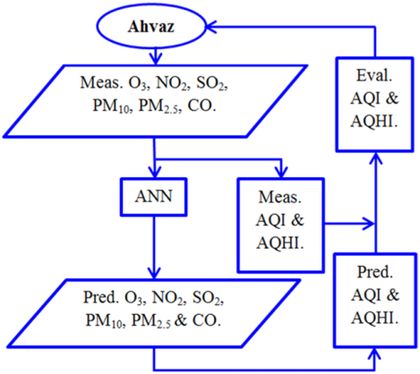
Graphical abstract

Introduction

Air pollution poses deleterious effects on people’s health, especially those in vulnerable populations such as children, elder women and men, and patients who suffer from respiratory and cardiovascular diseases (Naddafi et al. 2012; Nourmoradi et al. 2016). Air pollution also has detrimental effects on the environment, socioeconomics, agriculture, and politics (Zhang et al. 2008; Vlachokostas et al. 2010; Maghrabi et al. 2011; Hou et al. 2016). The following six criteria air pollutants are sufficiently harmful for humans and the environment that they are routinely monitored by the United States Environmental Protection Agency (US EPA), which has set National Ambient Air Quality Standards (40 CFR part 50) for these species: carbon monoxide, lead, nitrogen dioxide, ozone, particulate matter (PM₁₀ and PM_2.5), and sulfur dioxide. The EPA reports daily air quality conditions as an air quality index (AQI), which is calculated based on these criteria air pollutants (except lead). The air quality health index (AQHI), developed by Health Canada and Environment Canada (HCEC), is an analogous index considering PM_2.5, O₃, and NO₂.

Meteorology and emissions sources of pollutants are two basic factors influencing the aforementioned air quality indices and can be used in computational approaches to predict spatiotemporal pollutant profiles and air quality index values. Various applicable examples include the Community Multi-scale Air Quality (CMAQ) model, the Weather Research and Forecasting model with Chemistry (WRF-Chem), and artificial neural network (ANN) and fuzzy inference systems (Pokrovsky et al. 2002; Cai et al. 2009; Wang et al. 2010; Feng et al. 2015; Zhang et al. 2015, 2016). ANN approaches can enhance forecasting accuracy relative to previously used statistical procedures (Nagendra and Khare 2005). Types of ANN include the back-propagation neural network (BPNN) (Chen and Pai, 2015; Bai et al. 2016), multilayer perceptron (MLP) (Wang and Lu 2006; Duräo et al. 2016), radial basis function (RBF) (Lu et al. 2004; Iliyas et al. 2013), and adopted neuro-fuzzy inference systems (ANFIS) (Shahraiyni et al. 2015; Prasad et al. 2016). Among the earliest applications of ANN for air pollution, research was forecasting SO₂ levels in Slovenia (Boznar et al. 1993). More recent attempts of using ANN include combining remotely sensed aerosol optical depth (AOD) and meteorological data to estimate surface PM_2.5 levels (Gupta and Christopher 2009). Numerous studies have evaluated various aspects of PM_2.5 and PM₁₀ mass concentration in different areas such as Taiwan (Chang and Lee 2007), Italy (Ragosta and Gioscio 2009), New Zealand (Elangasinghe et al. 2014), the western Mediterranean (de Gennaro et al. 2013), India (Patra et al. 2016), Portugal (Russo et al. 2015), and China (Qin et al. 2014; Yao and Lu 2014).

In this study, we apply a ANN model approach to predict hourly criteria air pollutant concentrations (O₃, NO₂, SO₂, PM₁₀, PM_2.5, CO), daily AQI, and hourly AQHI. The analysis focuses on Ahvaz, Iran, which suffers from some of the worst air conditions globally owing to severe dust storms. It was recently reported to be the highest ranked city in terms of mean-annual PM₁₀ concentration on the Earth (372 μg m⁻³; Goudie 2014). The subsequent analysis focuses on model prediction comparisons to measurement data at four sites around Ahvaz, with attention given to how well diurnal profiles are reproduced.

Experimental methods

Study area

Ahvaz is the capital of Khuzestan province located close to the Persian Gulf in southwestern of Iran, and it contains the largest river of Iran (Karun) (Fig. 1). Its population is ~ 1.2 million and has an area of ~ 528 km² (Naimabadi et al. 2016). The climate in this region is hot and humid. This study makes use of hourly data collected between August 2009 and August 2010 by the Ahvaz Environmental Protection Organization (AEPO) and Ahvaz Meteorological Center. Samples were obtained using the beta attenuation procedure, which is often common at routine monitoring stations. Measurements of O₃, NO₂, CO, SO₂, and PMs were conducted, respectively, via the use of Beer–Lambert’s law, chemiluminescence, non-dispersive infrared spectroscopy, UV fluorescence, and beta radiation (Mazaheri Tehrani et al. 2015; Alizadeh-Choobari et al. 2016). Data related to pollutants concentration and meteorological parameters affecting the forecast of model, such as wind speed (m/s), ambient air temperature (°C), dew point (°C), rainfall (mm), and air pressure, are presented in Table 2. The four sampling locations for O₃, NO₂, PM₁₀, PM_2.5, SO₂, CO, and meteorology are shown in Fig. 1 (Naderi, Havashenasi, Mohite Zist, Behdasht).

Fig. 1.

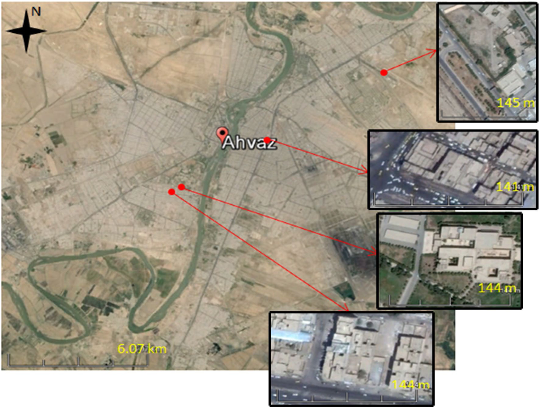
Map showing the location of four sites from which data were collected for criteria air pollutants in Ahvaz, Iran. Names of sites (from top to bottom) are Havashenasi (Meteorology), Naderi, Behdasht, and Mohit Zist (Maleki et al. 2016)

Table 2.

Range, mean, and standard deviation of input meteorological parameters and measured and predicted criteria air pollutant concentrations (WS wind speed, T temperature, T_d dew point, P air pressure, R rainfall)

Variable	Unit	Range	Mean	SD
Measured
WS	m s−1	[0.0–6.7]	1.1	1.0
T	°C	[3.0–50.2]	27.1	10.1
Td	°C	[−9.9 to 29.6]	9.8	5.4
P	hPa	[990.7–1025.2]	1009.3	8.1
R	mm	[0.0–34.0]	245.3a	1.6
O3	ppb	[0.2–567.8]	25.1	17.4
NO2	ppb	[0.1–692.7]	23.5	36.3
SO2	ppb	[0.0–488.3]	32.1	54.2
PM10	μg m−3	[8.0–6900.0]	284.3	421.3
PM2.5	μg m−3	[3.2–2760.0]	113.7	165.5
CO	ppm	[0.0–25.5]	1.6	2.2
Predicted
O3	ppb	[−8.3 to 547.0]	25.0	15.1
NO2	ppb	[−156.0 to 681.4]	23.2	31.1
SO2	ppb	[−11.3 to 480.2]	32.2	53.7
PM10	μg m−3	[−492.8 to 6889.6]	287.4	372.3
PM2.5	μg m−3	[−242.3 to 2422.4]	113.6	142.2
CO	ppm	[−1.3 to 23.6]	1.6	2.1

^aThis shows the accumulative volume of rainfall

Air pollution indexes

AQI is calculated using concentration data for PM, NO₂, SO₂, CO, and O₃. Index values differ among global cities owing to various levels of anthropogenic activity, potential sources of natural emissions, as well as transport patterns of pollutants. Values are classified as good (0–50, green), moderate (51–100, yellow), unhealthy for susceptible groups (101–150, orange), unhealthy (151–200, red), very unhealthy (201–300, purple), and hazardous (301–500, Maroon). As will be shown, AQI values exceed 500 in the study region. The general equation to calculate AQI is as follows:

$$I_{\text{p}}=\frac{I_{\text{Hi}}-I_{\text{Lo}}}{{\text{BP}}_{\text{Hi}}-{\text{BP}}_{\text{Lo}}}\left(C_{\text{p}}-{\text{BP}}_{\text{Lo}}\right)+I_{\text{Lo}}$$ (1)

where I_p=the index for pollutant p, C_p=the rounded concentration of pollutant p, BP_Hi=the breakpoint that is ≥ C_p, BP_Lo=the breakpoint that is ≤ C_p, I_Hi=the AQI value corresponding to BP_Hi, and I_Lo=the AQI value corresponding to BP_Lo.

AQHI presents the health risk of pollutants based on the following scale: low risk (1–3, blue), moderate risk (4–6, orange), high risk (7–10, red), and very high risk (> 10, black). The AQHI is calculated according to the following formula using 3-h average concentrations of O₃, NO₂, and PM_2.5 (El-Latef et al. 2018).

$$\text{AQHI}=\frac{1000}{10.4}*\left[\left({\text{e}}^{0.000537*O_3}-1\right)+\left({\text{e}}^{0.000871*N{O}_2}-1\right)+\left({\text{e}}^{0.000487*P{M}_{2.5}}-1\right)\right]$$ (2)

Artificial neural network

A neural network utilizes artificial neurons, which are the smallest units of data processing (Sadorsky 2006). The framework of a one-input system is demonstrated in Fig. 2. Equation 3 is used to quantify the output:

$$p=f\left(\sum _{i=1}^m{w}_i{x}_i\right)+b$$ (3)

$$\sigma \left(p\right)=\frac{1}{1+{\text{e}}^{-p}}$$ (4)

where b and w represent parameters that are set based on a selected activation function and type of learning algorithm. A number of different activation functions such as linear, sigmoid, and hyperbolic tangent can be used that for this study Sigmoid function was used (Eq. 4) (Alimissis et al. 2018; Elfwing et al. 2018).

Fig. 2.

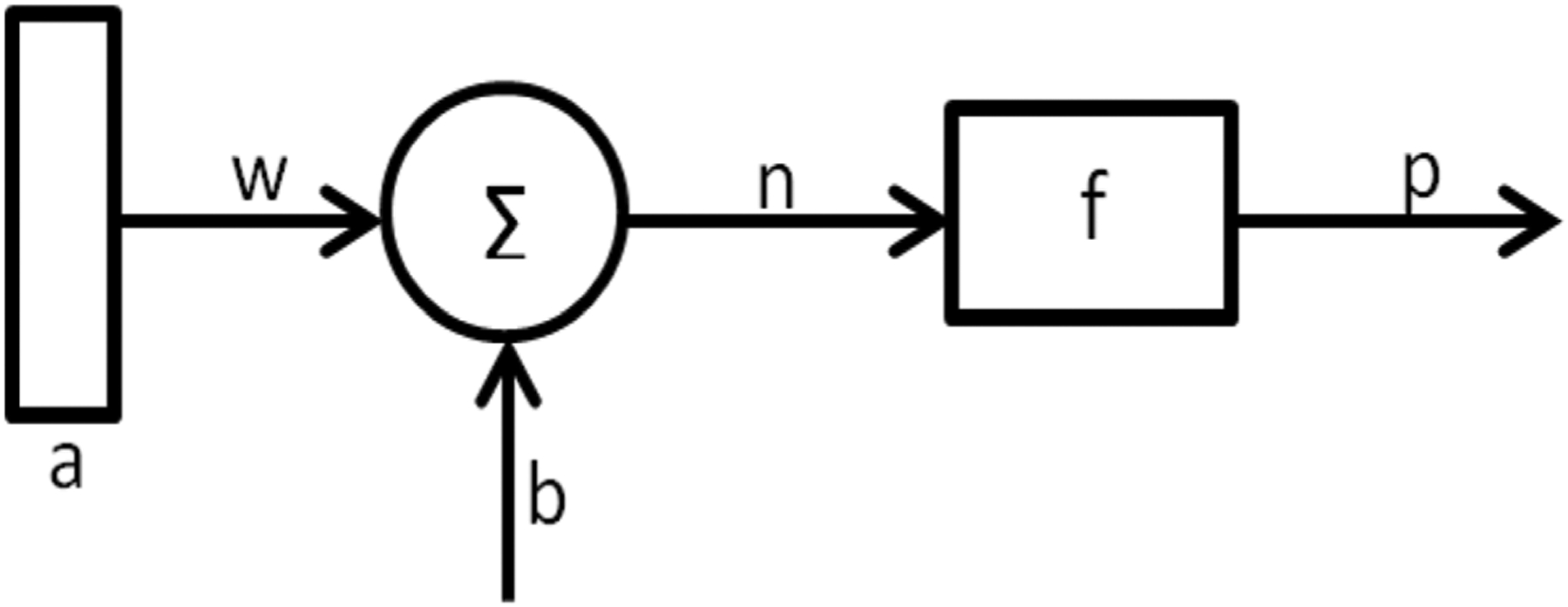
A one-input neuron system, where f is the activation function, and a, p, w, and b are the entrance data, outcome, weight, and neuron bias, respectively

Figure 3 depicts the ANN structure applied in this study. Nine input factors are used, with 30 nerve cells in the intermediate step leading to one outcome. The 30 neurons in the interior layer were identified through a trial-and-error process using between 6 and 60 nerve cells. It was necessary to determine what percentage of randomly selected data points from the available sample set needed to be assigned to training, validation, and testing in order to obtain the best agreement between predicted and measured concentrations. Points assigned to training are used for computations and updating the network weights and biases to train candidate algorithms. For evaluation of performance, Eqs. 5 and 6 are used to obtain linear correlation coefficients and RMSE, respectively:

$$R^2={\left(\frac{{\sum }_1^n\left[\left({\widehat{Y}}_i-{\overline{\widehat{Y}}}_i\right)*\left(Y_i-{\overline{Y}}_i\right)\right]}{{\left({\sum }_1^n\left[{\left({\widehat{Y}}_i-{\overline{\widehat{Y}}}_i\right)}^2*\left(Y_i-{\overline{Y}}_i\right)\right]\right)}^{0.5}}\right)}^2$$ (5)

$$\text{RMSE}=\sqrt{\frac{{\sum }_1^n{(\text{Meas}-\text{Pred})}^2}{n}}$$ (6)

where Y_i and Ȳ_i are the measured concentrations and average of measured concentrations for a pollutant, respectively. Ŷ_i and ${\overline{\widehat{Y}}}_i$ are predicted concentrations and average of predicted concentrations for a pollutant, respectively, n is the number of data values, Meas is the measured data, and Pred is the predicted data. The ideal value for R² and RMSE is 1 and 0, respectively (Ho et al. 2002).

Fig. 3.

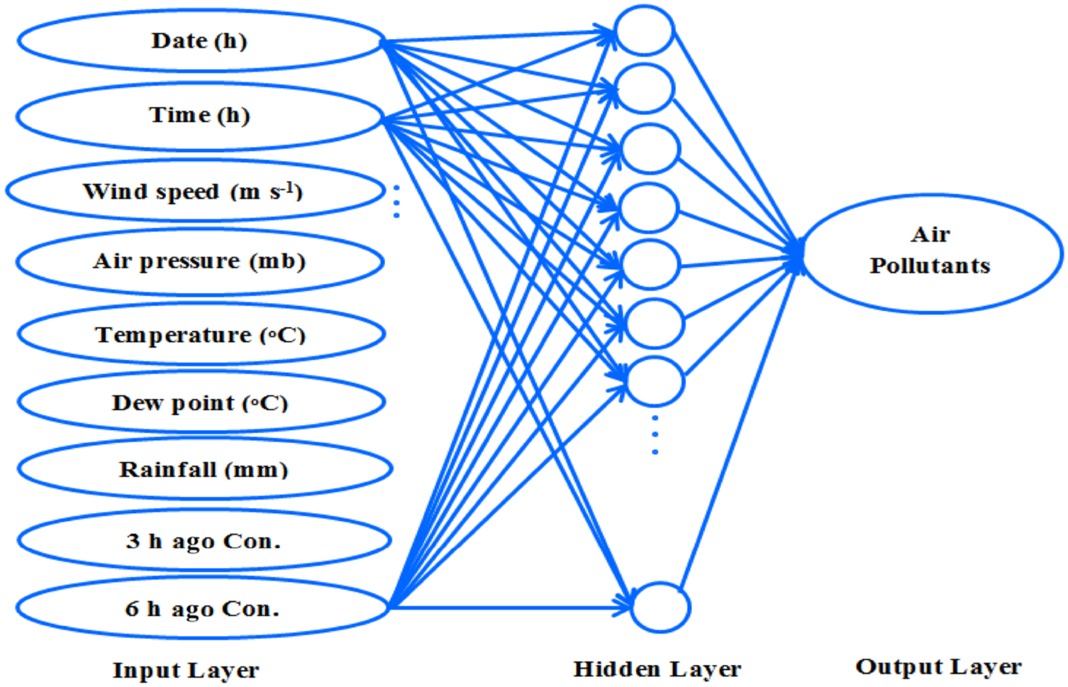
Structural diagram of ANN with nine inputs, one hidden layer (30 neurons), and one output. “3 h ago Con.” and ‘6 h ago Con.” refer to concentrations of a particular pollutant 3 and 5 h in advance of the time of the predicted concentration, respectively

Results and discussion

It was first necessary to determine under what conditions the best agreement could be attained between predicted and measured concentrations. The ANN was tested with having either 5% or 10% of data used for both validation and testing, with the remainder for training. When the total data used in the validation and testing stage decreased from 10 to 5% for the four air quality monitoring stations in Ahvaz, the average correlation coefficient (R) between measured and predicted concentrations (for all pollutants and sites combined) increased by 8.1% while RMSE decreased by 11.8% (Table 1).

Table 1.

Correlation coefficient (R) and root-mean square error (RMSE) when using 5% and 10% of data for validation and testing of criteria air pollutant concentrations for the four air quality monitoring stations in Ahvaz

Stations	O3 (ppb)		NO2 (ppb)		SO2 (ppb)		PM10 (μg m−3)		PM2.5 (μg m−3)		CO (ppm)
	R	RMSE	R	RMSE	R	RMSE	R	RMSE	R	RMSE	R	RMSE
5%
Naderi	0.88	2.8	0.89	4.0	0.83	12.3	0.91	236.6	0.91	80.3	0.87	0.6
Havashenasi	0.84	2.9	0.82	40.9	0.75	5.0	0.85	200.9	0.86	57.5	0.81	0.3
Mohite Zist	0.90	2.8	0.84	13.4	0.99	12.1	0.86	343.3	0.86	123.5	0.84	1.3
Behdasht	0.80	3.0	0.91	4.8	0.88	4.6	0.89	213.4	0.89	69.3	0.94	1.6
Average	0.86	2.9	0.87	15.8	0.86	8.5	0.88	248.5	0.88	82.6	0.87	1.0
10%
Naderi	0.82	8.2	0.85	19.4	0.82	11.9	0.87	298.3	0.87	80.6	0.85	0.5
Havashenasi	0.83	9.4	0.79	38.1	0.69	5.4	0.84	251.3	0.82	88.2	0.80	0.4
Mohite Zist	0.89	8.4	0.79	11.5	0.99	12.2	0.84	264.6	0.83	136.3	0.81	1.4
Behdasht	0.77	10.3	0.91	4.4	0.87	3.0	0.86	274.0	0.86	90.4	0.93	1.4
Average	0.77	9.1	0.80	18.3	0.83	8.1	0.85	272.0	0.84	98.9	0.74	1.0

Figure 4 shows the relationship between measured and predicted concentrations at all sites for different pollutants based on 5% of data for validation and testing stages. Among criteria air pollutants, SO₂ exhibited the best results at the Mohite Zist station (R = 0.99), while SO₂ yielded the worst performance at the Havashenasi station (R = 0.75). The lowest RMSE was for CO at the Havashenasi station (0.3), while the highest value was for PM₁₀ at the Mohite Zist station (360.5). The averages among all pollutants and sites combined for R and RMSE were 0.87 and 59.9, respectively.

Fig. 4.

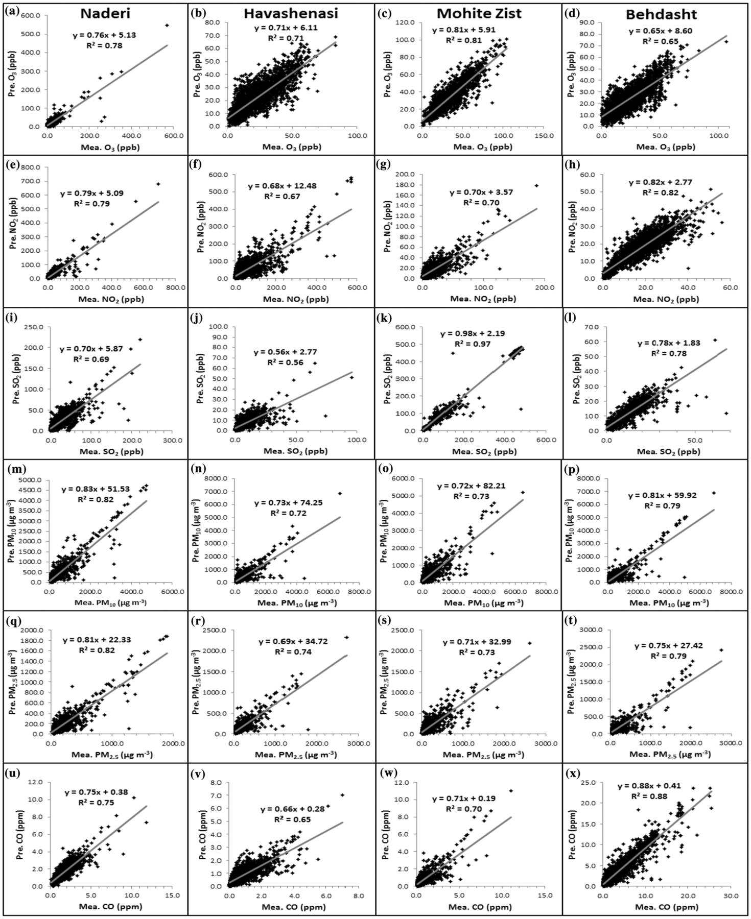
Scatterplots showing measured versus predicted concentrations for various pollutants in four stations based on 5% of data used for validation and testing. Data shown for panels in each column refer to the station shown at the top of that column

A comparison between measured and predicted pollutant concentrations of all four stations is presented in Table 2. When taking an average for all six pollutants, the range of variation for predicted levels increased by 3.4% as compared to measured values, whereas the standard deviation decreased by 10.2%. No difference was observed between the average of total predicted and measured pollutant concentrations. The widest range of values was for PM₁₀, while the lowest was for CO.

The diurnal concentration profile of measured and predicted pollutant concentrations at the four air quality monitoring stations in Ahvaz is presented in Fig. 5. Expectedly based on the results of Table 1, the diurnal profiles for the studied pollutants are similar between measurements and the model. O₃, PM₁₀, PM_2.5, and SO₂ exhibit minimum levels early in the morning and late night, with maximum values in between during the day. Diurnal variations for NO₂ and CO exhibit minimum values in the early morning and afternoon, and maximum levels before noon and at night.

Fig. 5.

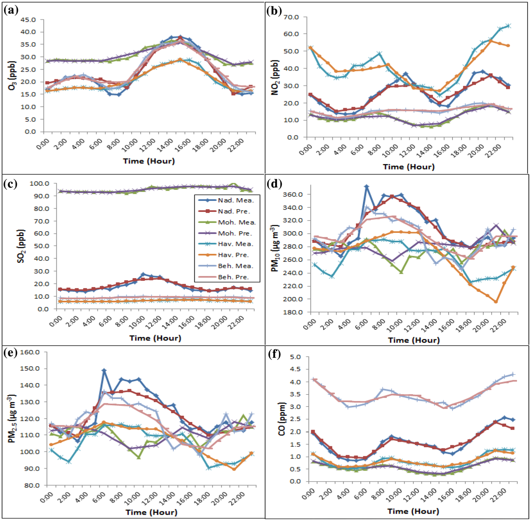
Measured and predicted diurnal average concentration of O₃ (a), NO₂ (b), SO₂ (c), PM₁₀ (d), PM_2.5 (e), and CO (f) for the four air quality monitoring stations

A comparison between calculated and predicted AQI is presented in Table 3 for the four sites in Fig. 1 and also for all four sites combined, representative of the entire city of Ahvaz. With regard to R² values, the ANN method was weak in terms of predicting AQI at the Naderi, Mohite Zist, and Behdasht stations, but it had acceptable performance (R² = 0.73) at the Havashenasi station. The cumulative percentage of days where the predicted AQI category did not match the measured one at Naderi, Havashenasi, Mohite Zist, and Behdasht stations and the bulk average of all sites as Ahvaz city was 49.6%, 38.1%, 61.3%, 48.5%, and 42.7%, respectively. Also, the number of days when at least one of the six pollutants exceeded its maximum limit at Naderi, Havashenasi, Mohite Zist, and Behdasht, and Ahvaz city was 28, 23, 31, 25, and 71, respectively.

Table 3.

Number (N) and percentage (%) of days when the measured AQI category does not match the predicted one (moderate (M), unhealthy for sensitive groups (UNSG), unhealthy (UN), very unhealthy (VUN) and hazardous (H¹ and H²)), in addition to correlation coefficient (R²) values for the relationship between measured and predicted AQI, and the days out of range (DOR) for measured AQI in Ahvaz

Stations	R2	M		UHSG		UH		VUH		H1		H2		Sum		DOR
		N	%	N	%	N	%	N	%	N	%	N	%	N	%	N	%
Naderi	0.003	-	-	55	15.1	73	20	16	4.4	23	6.3	14	3.8	171	49.6	28	7.7
Havashenasi	0.73	-	-	70	19.2	24	6.6	29	7.9	9	2.5	7	1.9	139	38.1	23	6.3
Mohite Zist	0.004	5	1.4	100	27.4	78	21.4	12	3.3	18	4.9	11	3	224	61.3	31	8.5
Behdasht	0.001	-	-	67	18.4	67	18.4	23	6.3	7	1.9	13	3.6	177	48.5	25	6.8
Ahvaz	0.07	-	-	3	0.8	54	14.8	33	9	36	9.9	30	8.2	156	42.7	71	19.5

The daily profile of AQI during the study period (August 2009–August 2010) is illustrated in Fig. 6. We assumed the upper limit of AQI was equal to 600 instead of 500. At the Havashenasi station, there were no significant fluctuations for AQI in November, December, and January. Averages of calculated AQI were 188, 178, 172, 180, and 240 at Naderi, Havashenasi, Mohite Zist, and Behdasht, and Ahvaz city, respectively, without considering (by ignoring) the assumed value of AQI for correspondent pollutants during the study period. As a result, the capability of ANN for predicting AQI increased when the number of out-of-range days related to correspondent pollutants (mostly PM₁₀ and PM_2.5 in Ahvaz) decreased. By considering the maximum level of AQI at all stations to describe Ahvaz’s AQI, the average of it in the city of Ahvaz was 1.34 times higher than mean AQI of air quality control stations.

Fig. 6.

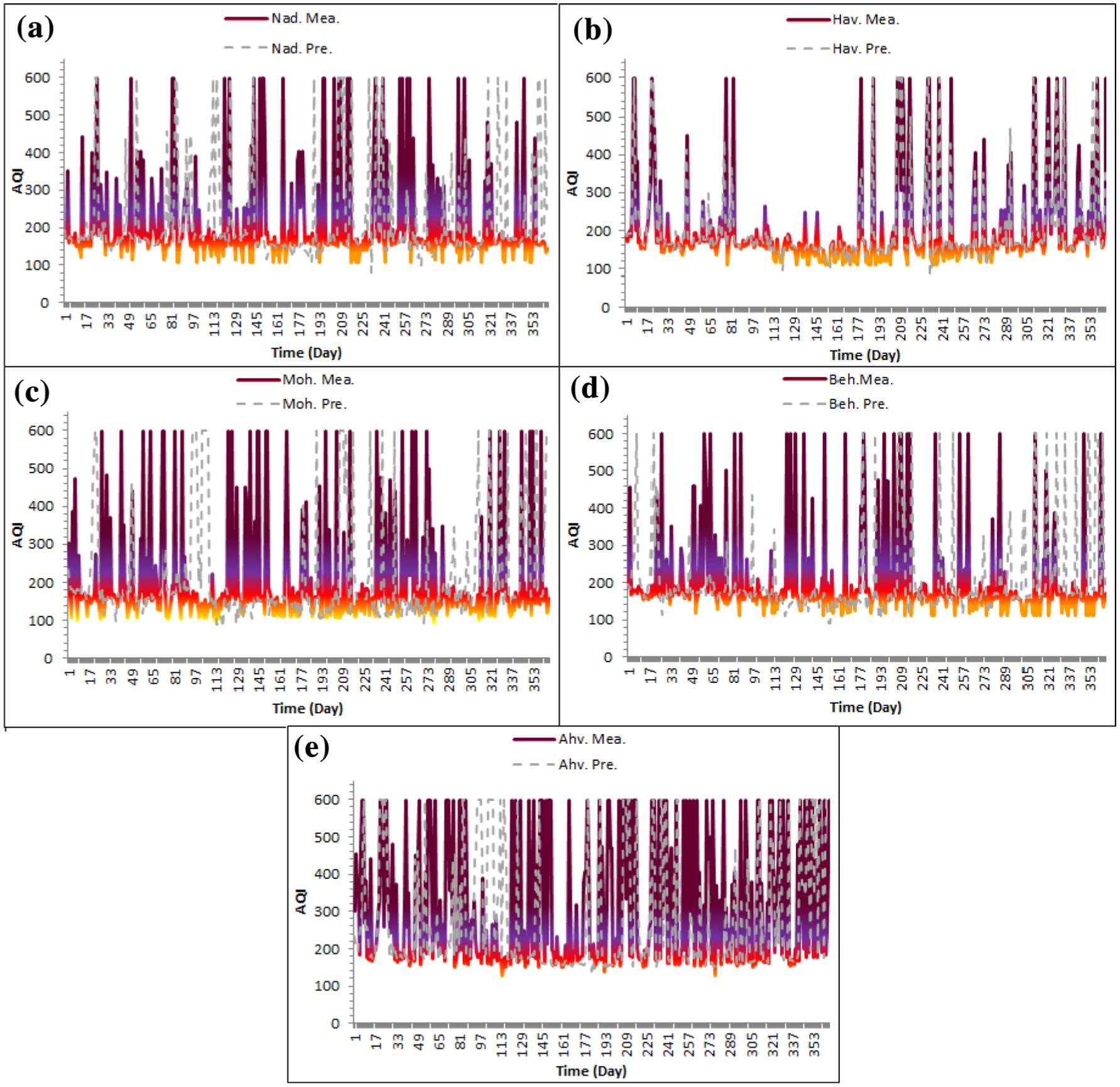
Time series of predicted and measured AQI for four air quality monitoring stations in Ahvaz, including all of them averaged, which is representative of the entire city of Ahvaz. Results are shown for the period between August 2009 and August 2010. Values are classified as good (0–50, green), moderate (51–100, yellow), unhealthy for susceptible groups (101–150, orange), unhealthy (151–200, red), very unhealthy (201–300, purple), and hazardous (> 301, Maroon)

A comparison between calculated and predicted AQHI is presented in Table 4. The R² value from the ANN method for predicting AQHI was 0.81, 0.70, and 0.78 at Naderi, Mohite Zist, and Behdasht, respectively, indicative of a decent level of performance. The Havashenasi station was an exception with a low R² value, which implies weak performance of the ANN to predict AQHI at this station. The percentage of hours with mismatches between predicted and measured AQHI at Naderi, Havashenasi, Mohite Zist, and Behdasht was 35.7%, 45.6%, 40.9%, and 37.8%, respectively. Also, the number of hours for AQHI being greater than or equal to 20, which is close to an AQI of 500, was 553, 677, 450, and 382 (out of a total of 8030) at Naderi, Havashenasi, Mohite Zist, and Behdasht, respectively.

Table 4.

Number (N) and percentage (%) of hours when the measured AQHI category does not match the predicted one (low (L), moderate (M), high (H) and very high (VH)), correlation coefficient (R²) value of measured and predicted AQHI and the hours greater and equal than 20 (HGE₂₀)

Stations	R2	L		M		H		VH		Sum		HGE20
		N	%	N	%	N	%	N	%	N	%	N	%
Naderi	0.81	112	1.4	1239	15.4	913	11.4	602	7.5	2866	35.7	553	6.9
Havashenasi	0.38	368	4.6	1689	21.0	931	11.6	677	8.4	3665	45.6	677	8.4
Mohite Zist	0.70	713	8.9	1336	16.6	852	10.6	381	4.7	3282	40.9	450	5.6
Behdasht	0.78	292	3.6	1417	17.6	864	10.8	466	5.8	3039	37.8	382	4.8

The temporal profile of calculated and predicted AQHI at the four stations over a span of 1 year (8760 h) is depicted in Fig. 7. On average, the calculated AQHI values at Naderi, Havashenasi, Mohite Zist, and Behdasht were 10, 10, 8, and 9, respectively. If there are many hours with AQHI ≥ 20, the capability of ANN to accurately predict AQHI decreases. Of note is that there was no significant fluctuation in Ahvaz during December and January for AQHI.

Fig. 7.

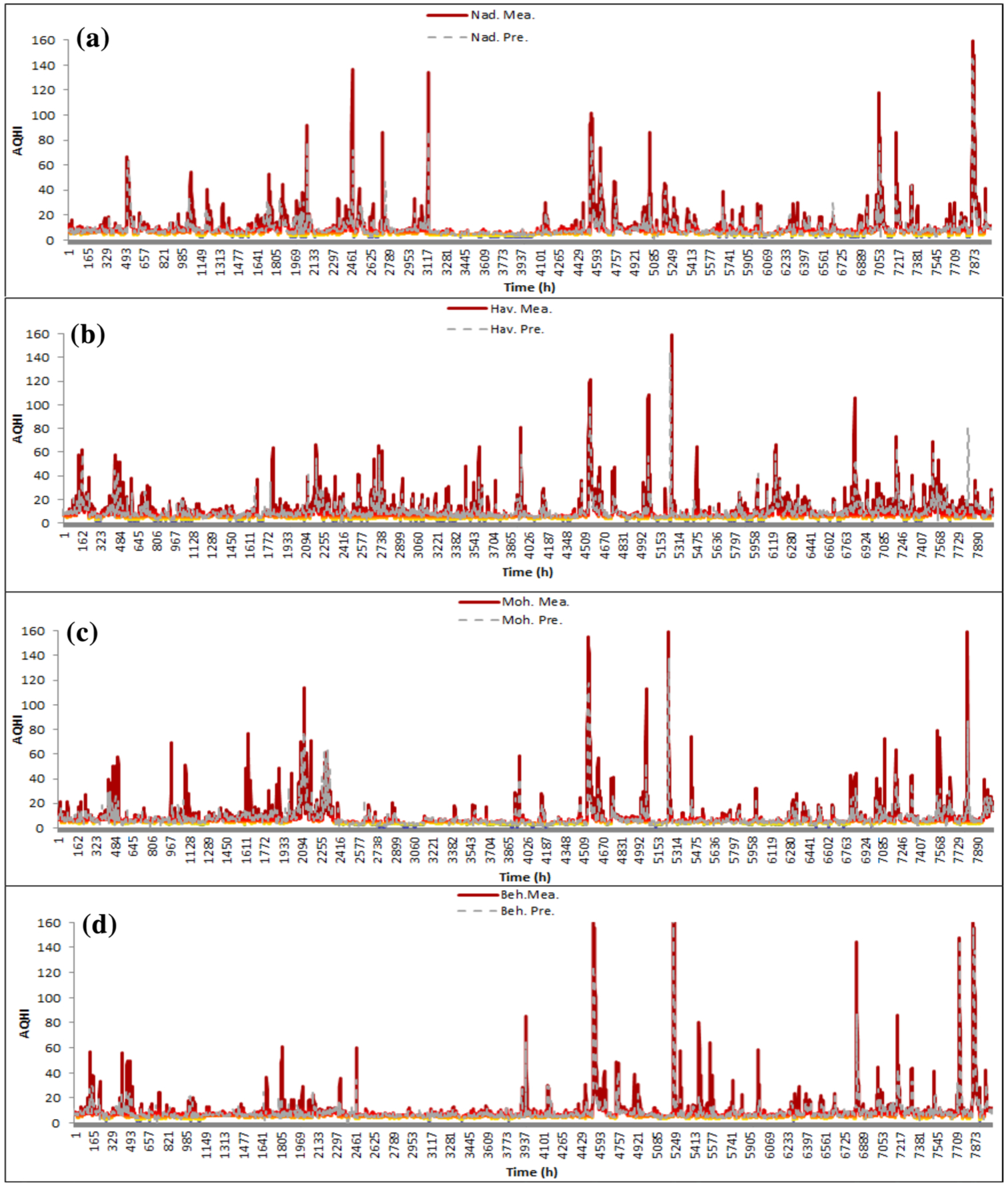
Predicted and measured AQHI variations for four air quality monitoring stations from August 2009 through August 2010 in Ahvaz

Conclusions

The overall correlation coefficient (R) for measured versus predicted pollutant concentrations for several sites in Ahvaz was shown to be 0.87 over the span of 1 year. The diurnal concentration profiles for both measured and predicted O₃, PM₁₀, PM_2.5, and SO₂ were similarly unimodal, while the variations for NO₂ and CO were bimodal. The critical aspect for the accuracy of ANN model is the number of high-polluted hours and days, respectively, for AQHI and AQI.

We conclude that authorities of urban air quality, practitioners, and decision makers can apply ANN to forecast the spatial–temporal profile of pollutant concentrations and air quality indices during power outage and wrong and negative records of pollutants. The study proposes that the ANN models could be used as an effective alternative in air pollution spatial interpolation and the representativeness of the air monitoring networks by providing data at currently unmonitored locations and thus eliminating the requirement of a relatively high number of monitoring stations for describing the air pollution spatial variability (Alimissis et al. 2018). Further research is recommended to compare the efficiency and potency of ANN with numerical, computational, and statistical models to enable managers to select an appropriate toolkit for better decision making in field of urban air quality.

References

- Alimissis A, Philippopoulos K, Tzanis CG, Deligiorgi D (2018) Spatial estimation of urban air pollution with the use of artificial neural network models. Atmos Environ 191:205–213 [Google Scholar]
- Alizadeh-Choobari O, Bidokhti AA, Ghafarian P, Najafi MS (2016) Temporal and spatial variations of particulate matter and gaseous pollutants in the urban area of Tehran. Atmos Environ 141:443–453 [Google Scholar]
- Bai Y, Li Y, Wang X, Xie J, Li C (2016) Air pollutants concentrations forecasting using back propagation neural network based on wavelet decomposition with meteorological conditions. Atmos Pollut Res 7(3):557–566 [Google Scholar]
- Boznar M, Lesjak M, Mlakar P (1993) A neural network-based method for short-term predictions of ambient SO2 concentrations in highly polluted industrial areas of complex terrain. Atmos Environ Part B Urban Atmos 27(2):221–230 [Google Scholar]
- Cai M, Yin Y, Xie M (2009) Prediction of hourly air pollutant concentrations near urban arterials using artificial neural network approach. Transp Res Part D Transp Environ 14(1):32–41 [Google Scholar]
- Chang SC, Lee CT (2007) Assessment of PM10 enhancement by yellow sand on the air quality of Taipei, Taiwan in 2001. Environ Monit Assess 132:297–309 [DOI] [PubMed] [Google Scholar]
- Chen L, Pai T-Y (2015) Comparisons of GM (1, 1), and BPNN for predicting hourly particulate matter in Dali area of Taichung City, Taiwan. Atmos Pollut Res 6(4):572–580 [Google Scholar]
- de Gennaro G, Trizio L, Di Gilio A, Pey J, Perez N, Cusack M, Alastuey A, Querol X (2013) Neural network model for the prediction of PM10 daily concentrations in two sites in the Western Mediterranean. Sci Total Environ 463:875–883 [DOI] [PubMed] [Google Scholar]
- Durao RM, Mendes MT, Pereira MJ (2016) Forecasting O3 levels in industrial area surroundings up to 24 h in advance, combining classification trees and MLP models. Atmos Pollut Res 7(6):961–970 [Google Scholar]
- Elangasinghe MA, Singhal N, Dirks KN, Salmond JA, Samarasinghe S (2014) Complex time series analysis of PM10 and PM2.5 for a coastal site using artificial neural network modelling and k-means clustering. Atmos Environ 94:106–116 [Google Scholar]
- Elfwing S, Uchibe E, Doya K (2018) Sigmoid-weighted linear units for neural network function approximation in reinforcement learning. Neural Netw 107:3–11 [DOI] [PubMed] [Google Scholar]
- El-Latef EMA, Zaki GR, Issa AI (2018) Traffic air quality health index in a selected street, Alexandria. J High Inst Public Health 48(2):67–76 [Google Scholar]
- Feng X, Li Q, Zhu Y, Hou J, Jin L, Wang J (2015) Artificial neural networks forecasting of PM 2.5 pollution using air mass trajectory based geographic model and wavelet transformation. Atmos Environ 107:118–128 [Google Scholar]
- Goudie AS (2014) Desert dust and human health disorders. Environ Int 63:101–113 [DOI] [PubMed] [Google Scholar]
- Gupta P, Christopher SA (2009) Particulate matter air quality assessment using integrated surface, satellite, and meteorological products: 2. A neural network approach. J Geophys Res Atmos 114(D14) [Google Scholar]
- Ho S, Xie M, Goh T (2002) A comparative study of neural network and Box-Jenkins ARIMA modeling in time series prediction. Comput Ind Eng 42(2):371–375 [Google Scholar]
- Hou Q, An X, Tao Y, Sun Z (2016) Assessment of resident’s exposure level and health economic costs of PM 10 in Beijing from 2008 to 2012. Sci Total Environ 563:557–565 [DOI] [PubMed] [Google Scholar]
- Iliyas SA, Elshafei M, Habib MA, Adeniran AA (2013) RBF neural network inferential sensor for process emission monitoring. Control Eng Pract 21(7):962–970 [Google Scholar]
- Lu W-Z, Wang W-J, Wang X-K, Yan S-H, Lam JC (2004) Potential assessment of a neural network model with PCA/RBF approach for forecasting pollutant trends in Mong Kok urban air, Hong Kong. Environ Res 96(1):79–87 [DOI] [PubMed] [Google Scholar]
- Maghrabi A, Alharbi B, Tapper N (2011) Impact of the March 2009 dust event in Saudi Arabia on aerosol optical properties, meteorological parameters, sky temperature and emissivity. Atmos Environ 45(13):2164–2173 [Google Scholar]
- Maleki H, Sorooshian A, Goudarzi G, Nikfal A, Baneshi MM (2016) Temporal profile of PM10 and associated health effects in one of the most polluted cities of the world (Ahvaz, Iran) between 2009 and 2014. Aeolian Res 22:135–140 [DOI] [PMC free article] [PubMed] [Google Scholar]
- Mazaheri Tehrani A, Karamali F, Chimehi E (2015) Evaluation of 5 air criteria pollutants Tehran, Iran. Int Arch Health Sci 2(3):95–100 [Google Scholar]
- Naddafi K, Hassanvand MS, Yunesian M, Momeniha F, Nabizadeh R, Faridi S, Gholampour A (2012) Health impact assessment of air pollution in megacity of Tehran, Iran. Iran J Environ Health Sci Eng 9(1):1. [DOI] [PMC free article] [PubMed] [Google Scholar]
- Nagendra SS, Khare M (2005) Modelling urban air quality using artificial neural network. Clean Technol Environ Policy 7(2):116–126 [Google Scholar]
- Naimabadi A, Ghadiri A, Idani E, Babaei AA, Alavi N, Shirmardi M, Khodadadi A, Marzouni MB, Ankali KA, Rouhizadeh A (2016) Chemical composition of PM 10 and its in vitro toxicological impacts on lung cells during the Middle Eastern Dust (MED) storms in Ahvaz, Iran. Environ Pollut 211:316–324 [DOI] [PubMed] [Google Scholar]
- Nourmoradi H, Khaniabadi YO, Goudarzi G, Daryanoosh SM, Khoshgoftar M, Omidi F, Armin H (2016) Air quality and health risks associated with exposure to particulate matter: a cross-sectional study in Khorramabad, Iran. Health Scope 5(2):e31766 [Google Scholar]
- Patra AK, Gautam S, Majumdar S, Kumar P (2016) Prediction of particulate matter concentration profile in an opencast copper mine in India using an artificial neural network model. Air Qual Atmos Health 9:697–711 [Google Scholar]
- Pokrovsky OM, Kwok RH, Ng C (2002) Fuzzy logic approach for description of meteorological impacts on urban air pollution species: a Hong Kong case study. Comput Geosci 28(1):119–127 [Google Scholar]
- Prasad K, Gorai AK, Goyal P (2016) Development of ANFIS models for air quality forecasting and input optimization for reducing the computational cost and time. Atmos Environ 128:246–262 [Google Scholar]
- Qin SS, Liu F, Wang JZ, Sun BB (2014) Analysis and forecasting of the particulate matter (PM) concentration levels over four major cities of China using hybrid models. Atmos Environ 98:665–675 [Google Scholar]
- Ragosta M, Gioscio G (2009) Neural network model for forecasting atmospheric particulate levels. Chem Environ Impact Health Eff, Aerosols, pp 149–160 [Google Scholar]
- Russo A, Lind PG, Raischel F, Trigo R, Mendes M (2015) Neural network forecast of daily pollution concentration using optimal meteorological data at synoptic and local scales. Atmos Pollut Res 6:540–549 [Google Scholar]
- Sadorsky P (2006) Modeling and forecasting petroleum futures volatility. Energy Econ 28(4):467–488 [Google Scholar]
- Shahraiyni HT, Sodoudi S, Kerschbaumer A, Cubasch U (2015) A new structure identification scheme for ANFIS and its application for the simulation of virtual air pollution monitoring stations in urban areas. Eng Appl Artif Intell 41:175–182 [Google Scholar]
- Vlachokostas C, Nastis S, Achillas C, Kalogeropoulos K, Karmiris I, Moussiopoulos N, Chourdakis E, Banias G, Limperi N (2010) Economic damages of ozone air pollution to crops using combined air quality and GIS modelling. Atmos Environ 44(28):3352–3361 [Google Scholar]
- Wang D, Lu W-Z (2006) Forecasting of ozone level in time series using MLP model with a novel hybrid training algorithm. Atmos Environ 40(5):913–924 [Google Scholar]
- Wang F, Chen D, Cheng S, Li J, Li M, Ren Z (2010) Identification of regional atmospheric PM 10 transport pathways using HYSPLIT, MM5-CMAQ and synoptic pressure pattern analysis. Environ Model Softw 25(8):927–934 [Google Scholar]
- Yao L, Lu N (2014) Spatiotemporal distribution and short-term trends of particulate matter concentration over China, 2006–2010. Environ Sci Pollut R 21:9665–9675 [DOI] [PubMed] [Google Scholar]
- Zhang M, Song Y, Cai X, Zhou J (2008) Economic assessment of the health effects related to particulate matter pollution in 111 Chinese cities by using economic burden of disease analysis. J Environ Manag 88(4):947–954 [DOI] [PubMed] [Google Scholar]
- Zhang L, Wang T, Lv M, Zhang Q (2015) On the severe haze in Beijing during January 2013: unraveling the effects of meteorological anomalies with WRF-Chem. Atmos Environ 104:11–21 [Google Scholar]
- Zhang Y, Zhang X, Wang L, Zhang Q, Duan F, He K (2016) Application of WRF/Chem over East Asia: part I. Model evaluation and intercomparison with MM5/CMAQ. Atmos Environ 124:285–300 [Google Scholar]