DenseCNN: A Densely Connected CNN Model for Alzheimer's Disease Classification Based on Hippocampus MRI Data

Abstract

Alzheimer's Disease (AD) is a common type of dementia, affecting human memory, language ability and behavior. Hippocampus is an important biomarker for AD diagnosis. Previous hippocampus-based biomarker analyses mainly focused on volume, texture and shape of the bilateral hippocampus. 3D convolutional neural networks (CNNs) can understand and extract complex morphology features from Magnetic resonance imaging (MRI) and have recently been developed for hippocampus-based AD classification. However, existing CNN models often have highly complex structures and require large amounts of training data. Here we propose an accurate and lightweight Densely Connected 3D convolutional neural network (DenseCNN) for AD classification based on hippocampus segments. DenseCNN was trained on 746 and tested on 187 pairs of hippocampus from Alzheimer's Disease Neuroimaging Initiative (ADNI) databases. DenseCNN has an average accuracy of 0.898, sensitivity of 0.985, specificity of 0.852, and area under curve (A UC) of0.979, which are better than or comparable to state-of-art approaches.

Introduction

Alzheimer's Disease (AD) is a common type of dementia among elderly individuals. It causes the death of brain cells and brain atrophy and its symptoms include memory loss, language disability, mood swings, among others. Recorded number of deaths from AD in the United States was 83,493 in 2010, making it one of the leading causes of death in the elderly, and the number of people with Alzheimer's disease is expected to be 13.8 million by 2050¹.

AD is highly complex and heterogeneous, therefore accurate and less invasive biomarkers and tools for early diagnosis are needed. Many diagnostic methods for AD have been developed, including definitive diagnosis at postmortem; positron emission tomography (PET)² with b-amyloid or Tau specific radioligands; immunoassays in cerebrospinal fluid (CSF)³; Magnetic resonance imaging (MRI) to detect structural defects due to neurodegeneration, like localized thinning of cortical gray matter or loss of hippocampal volume; Structural MRI and 18-F Fluorodeoxyglucose (FDG) PET to recognize patterns of tissue loss and cerebral glucose Hypometabolism. While CSF sampling requires lumbar puncture and PET scans involve exposure to radioactivity, MRI is less invasive.

The Alzheimer's Disease Neuroimaging Initiative (ADNI) is a longitudinal multicenter study designed to develop clinical, imaging, genetic, and biochemical biomarkers for the early detection and tracking of AD⁴. Researchers have been using ADNI databases to build diagnosis tools of genetic, genomic, biochemical, and image features. N. Schuff et al. demonstrated that ApoE is highly related to AD and it has become a major genetic biomarker⁵. Features extracted from brain MRI, such as volume, cortical thickness and hippocampus shape have been used to diagnose AD⁶. Oskar Hansson et al. used CSF and PET from ADNI to predict clinical progression of mild cognitive impairment (MCI)⁷.

Deep learning or deep neural networks (DNN) has been increasingly applied in the field of biomedical image-based diagnosis. U-net, which is a neural network comprised of down sampling layers and up sampling layers, is widely used for biomedical image segmentation⁸. Deep Mind has used deep convolutional neural networks (CNN) for lung cancer screening based on low-dose chest computed tomography ⁹. Unsupervised DNN has been used as an Autoencoder so that high dimensional features of brain MRI can be compressed to low dimensional features, so that supervised DNN model can be built on low dimensional features to classify AD and normal controls (CN)¹⁰. CNN has shown its advantages in computer vision tasks since AlexNet in 2012¹¹. However Deep CNN suffers from degradation since adding more layers often lowers accuracy. Kaiming He et al. in 2015 introduced Residual blocks (ResBlock) into CNN model¹². The key to ResBlock is that a shortcut connects the input of the first convolutional layer and the output of the second convolutional layer, which can pass low level features to later layers in order to overcome the degradation problem in Deep CNN models. Gao Huang et al. proposed Densely Connected Convolutional Networks (DenseNet)¹³ of multiple Dense Blocks in order to significantly reduce parameters.

Hippocampus is a major component of the human brain that plays significant roles in both short- and long-term memory. Hippocampal atrophy is an important biomarker for AD diagnosis. A number of machine learning models have been developed to classify AD based on hippocampus imaging data. Olfa et al. extracted image features from Hippocampus, and built models based on Support Vector Machines(SVM) and Bayesian classifier¹⁴ . Ruoxuan Cui et al developed 3-Dimensional convolutional neural networks(3D-CNN) to classify AD and CN¹⁵. Hongming Li et al used 3D residual CNN to extract deep features of the hippocampus, then built a time-to-event model to predict mild cognitive impairment (MCI) progressing to AD¹⁶. Manhua Liu et al. proposed a multi-model CNN AD classifier, which used ResBlock residual block and Dense block in one single model¹⁷. Previous CNN models often have sophisticated structures, for example residual CNN and multi-model CNN heavily relied on feature engineering and required large amounts of training data, the latter is often the bottleneck in biomedical field. Overfitting can happen in Deep and complex CNN models, when the model structures are complex and training data are limited.

In this study, we propose a light-weight, densely connected 3D-CNN model (DenseCNN) for classifying AD from control normal (CN) based on hippocampus segmentations from ADNI. DenseCNN is densely connected with features from all levels, therefore no particular feature engineering is needed. DenseCNN is lightweight with fewer convolutional kernels, relatively simple structure and fewer total parameters. It does not heavily rely on data augmentation and is fast in training and predicting. For preparing the training and testing data, we leveraged the latest deep learning hippocampus segmentation tool (Hippmapper) ¹⁸ and the segmentation results were further manually quality controlled. Compared to previous studies of MRI-based AD classification CNN models, DenseCNN is robust with simpler structure and fewer parameters and was trained on more high-quality training data. When tested on a testing dataset of 2 to 7 times larger than previous studies, our model reached a high accuracy of 0.89, sensitivity of 0.985, specificity of 0.852 and area under curve (AUC) of 0.979, which are better than or are comparable to several state-of-art CNN models by Olfa¹⁴, Ruoxuan¹⁵, Hongming¹⁶, Manhau¹⁷ et al].

2. Method

2.1. Data selection

We obtained data from the ADNI (http://adni.loni.usc.edu). The MRI data is T1-weighted structural from initial screening or baseline, including ADNI 1,2/GO and 3. Screening visit screening visit consists of a list of assessments(including imaging) to evaluate whether a participant should be included in ADNI. After passing screening, baseline assessment collects more biomarkers from participants. Most participants have the same diagnosis in screening and baseline. If a participant has both screening and baseline scans, we will choose the baseline one, as baseline diagnosis is considered to be more accurate. After hippocampus segmentation, we have 326 AD subjects, 607 control normal (CN) subjects and 544 Mild Cognitive Impairment (MCI) subjects, totaling 1477 hippocampus segmentations. In this study, we focused on classifying AD from CN, therefore AD and CN subjects were used to train our residual 3D-CNN model. Most MCI and AD cases have brain atrophy and share similar imaging features. Classifying AD and MCI via MRI is often more difficult with moderate accuracy of 70%-80% and may require features other than imaging features. While classifying AD and MCI via MRI is not the focus of this study, we are developing models based on MRI and other data to classify subjects into AD, MCI and CN.

2.2. Hippocampus segmentation

Hippmapper, a deep learning based hippocampal segmentation tool¹⁸, can segment hippocampus from T1-weighted raw MRI. It is the 3D version of U-net and has two stages: firstly, the tool finds the location of the hippocampus and generates bounding boxes; secondly, the hippocampus is extracted from the bounding boxes. It has been shown to have better segmentation results than traditional machining learning tools, such as FreeSurfer, in all metrics¹⁸.

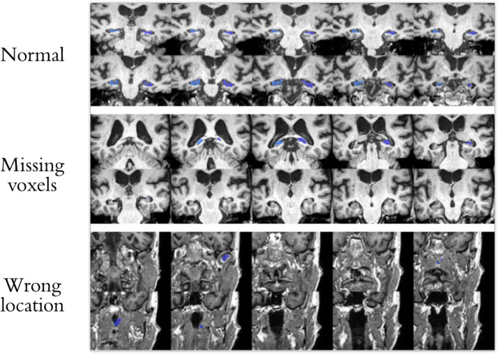
Accurate hippocampus segmentation data is the key to brain MRI-based classification models for AD, therefore we further manually checked all segmentation results from Hippmapper. Segmentations with following conditions were removed: segmentations from wrong sections of the brain; segmentations with noticeable missing voxels; the raw MRI data is not clear or has other defects. Examples of removed subjects are shown in Figure1. Around 5% of the initial segments were excluded from our dataset. During our experiments, we found that without this step of manual curation, the accuracy of our model was significantly lower as compared to models built on manually curated data.

2.3. 2.3. Data preprocess and augmentation

After segmentation, we had a list of masks for the location of the hippocampus in raw MRI, which have the same dimensions as the raw image. The right and left masks were separated in order to remove voxels with 0 value between the left and right hippocampus. The left and right hippocampus were extracted by multiplying right and left masks, metrics only consisting of 1 and 0 voxels, with the raw image metrics. We then removed slices containing only 0 value voxels, reducing the size of a hippocampus to the dimension of (48, 60, 46). All voxels were normalized to the scale of 0 - 1, which is a common step for training a CNN model¹⁹. This normalization step reduces gradients in model training, decreases the chance of overflow, and improves training speed.

A series of augmentations were then applied to the preprocessed data. The input size (48*60* 46) to our model is comparable to that of 2D computer vision models (256*256, 512*512), which could have over 100 layers. In 2D computer vision tasks, models are often trained on large datasets(ImageNet 14 million,CIFAR-10 60,000)²⁰. Deep CNN models could contain millions of trainable parameters. Large numbers of parameters training on limited data often leads to overfitting. For our task of training 3D CNN models, augmentation to enlarge training data is crucial. Each hippocampus segment for training was moved along the x, y and z axis, 6 directions in total, based on the method from previous studies ²¹. The training dataset is 6 times larger than original data after translational change, totaling 5222 subjects. We did not apply rotation, zoom-in or zoom-out to the original dataset, since hippocampus volume and orientations are important features and play an important role in AD diagnosis.

2.4. 2.4 DenseCNN

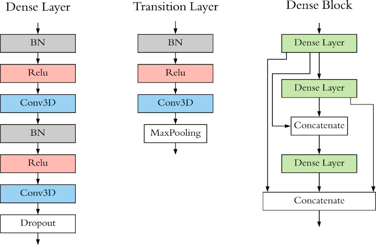
DenseCNN (Figure 2) has 3 dense layers, with each layer consisting of 2 convolutional layers, combined with Batch normalization (BN)²² layers and Relu activation layers. Transition Layers end with a Max Pooling layer to decrease the size of input data. The general dense connectivity was shown in eq. (1), where x0, x1, ... xl are the feature map for layers 0 to l and H() could be any non-linear transformation in the CNN.

$$xl=Hl([x0,x1,\dots xl-1])$$

Figure 2. Structure of Dense Layer, Transition Layer and Dense Block of Dense CNN.

In our case, the first convolutional layer used 1^1x1 size convolutional kernels(filter), while the second filter used filters with a size of 3x3x3 and had a stride of 1x1x1. In the Dense Block, the output of the first dense layer was concatenated with output of the second and third dense layers; the output of the second dense layer was concatenated with the third dense layer. Dropout layers²³ were used in our model to reduce overfitting.

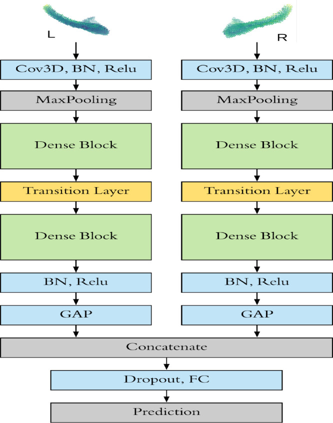
DenseCNN model has two streams for left and right hippocampus segments correspondingly (Figure 3). Each stream has an initial 3D convolutional layer followed by a BN layer and a Relu activation layer, extracting low level image features. Then a Max pooling was used to ignore 0 voxels on the edges of the input data and reduce the data size. Two Dense Blocks and a Transition Layer were stocked in each stream, using 8 and 16 filters correspondingly. At the end of each stream is a global average pooling (GAP) layer, which compresses high dimensional image features to 1-Dimensional features. After the GAP layer, two streams were merged followed by a dropout layer. Finally, a fully connected layer and a SoftMax layer were used for generating prediction.

Figure 3. The architecture of DenseCNN.

2.5. Validation

A total of 326 AD subjects and 607 CN subjects were used in this study. 5-fold cross validation was used in our study. Each time, 4 folds (746 subjects) were used for training and 1-fold (65 AD, 122 CN) for validation. Average classification accuracy, sensitivity, and precision of the 5 folds, receiver operating characteristic (ROC) curve, and area under ROC curve (AUC) were used as evaluation metrics.

2.6. Comparison

We compared DenseCNN with previous hippocampus-based CNN AD classification models, including Feature Based model, Plain 3D-CNN, Residual 3D CNN and Multi-model 3D CNN, described in the introduction. Classification accuracy, sensitivity, precision, and AUC were compared.

We examined the performance of DenseCNN with various depth and complexity and experimented with building models with different numbers of Dense Blocks and filters. A Transition Layer was also added into the model when an extra Dense Block was necessary. We tried Dense Blocks ranging from 1-4 and filters ranging from 4-64. Among those trails, we chose 4 models for comparison: 1. model with 3 Dense Blocks and has (8,16,32) filters in each Dense Block; 2. model with 3 blocks and has (6,12,12) filters; 3 model with 2 blocks and has (6,12)filters; 4. model with 2 blocks and has (12,24) filters. These comparison models have trainable parameters ranging from 140,682 to 1,021,074, which provided a wide-range coverage of model complexity.

Experiment platform and parameters

The segmentation process and model training were conducted on a NVIDIA GeForce GTX 1080 ti GPU with 11 GB memory. The model was implemented by Keras with the TensorFlow backend. RMSprop was chosen as the optimizer in the early stage of training. Once the model reached 80% accuracy, the optimizer was switched to Gradient Descent with Momentum for final fine turning. L2 regularization was used to reduce overfitting. We experimented with a wide range of hyperparameter values and different structures of models.

Result

2.7. 4.1. Performance Comparison of DenseCNN, Feature Based method, Plain 3D-CNN and Multi-model CNN

We computed the average performance from 5-fold cross validating. The model has achieved of an average accuracy of 0.891, sensitivity of 0.985, specificity of 0.852 and AUC of 0.979. We compared DenseCNN with previous methods (Table 1). In summary, our model achieved an overall best performance among all the previous models based on AUC and sensitivity measures. ResNet had an accuracy of 90.0% and is 0.2% higher than DenseCNN, however our model was evaluated on a test dataset of two times larger than ResNet (187 vs 63 subjects). The performances of previous studies were measured on test datasets consisting of 27 to 89 subjects. On the other hand, DenseCNN was evaluated on a test dataset of 187 subjects (Table 1), indicating that our performance measures are more robust.

Table 1. Performance Comparison of DenseCNN, Feature Based method, Plain 3D-CNN and Multi-model CNN.

Method	ACC	SEN	SPE	AUC	Number of test subjects
Olfa et al. 2014 Feature Based	85.0	76.0	81.0	-	27(15AD 12CN)
Ruoxuan et al. 2018 Plain 3D-CNN	87.0	79.38	93.22	86.41	46(20AD 26CN)
Hongming et al. 2019 ResNet	90.0	-	-	95.6	63(26AD 37NC)
Manhua et al. 2020 Multi-model CNN	88.9	86.6	90.8	92.5	89(45AD 44NC)
DenseCNN	89.8	98.5	85.2	97.9	187(65AD 122NC)

2.8. 4.2. Performance comparison of DenseCNNs with different architectures

We built DenseCNN with different architectures and compared their performances (Table 2). The Filters column in Table 2 shows the corresponding numbers of filters in each Dense Block. For example, a model with 3 Dense Blocks has 8 filters in the first block, 16 in second block, 32 in the third, and 1,021,074 trainable parameters in total. The lightest model has only 140,682 trainable parameters and has the lowest accuracy, demonstrating that an overly simplified models may be highly biased. The model with the most parameters (1,021,074) has the lowest AUC of 0.846, demonstrating that complex CNN models may be highly variable. The best performance was achieved for DenseCNN with 243,090 parameters.

Table 2. Comparison of DenseCNNs with different number of Dense Blocks and filters.

Total parameters	number of dense blocks	Filters	ACC	SEN	SPE	AUC
1,021,074	3	8,16,32	83.4	67.7	91.8	84.6
270,546	3	6,12,12	86.6	93.8	82.8	96.7
140,682	2	6,12	81.8	73.8	86.1	88.7
532,434	2	12,24	82.4	75.4	86.1	89.3
243,090	2	8, 16	89.8	98.5	85.2	97.9

Although shortcuts in Dense Block can pass low level feature to later layers in the same block, low level features may not be able to flow to all Dense Blocks. Models with 3 Dense Blocks were ended up with 21 convolutional layers, which may be too deep for any small size hippocampus (48,60,46). The model with one Dense Block had worse performance than plain CNN models. During our experimentation, we found that models with 2 Blocks worked the best. The number of Filter is also a significant performance factor. We followed the guideline from the original Densenet¹³ and Resnet¹² and doubled the filter number when max pooling was applied. Therefore, filters in later layers are decided by the filter number in the first Dense block. The choice of an appropriate number of filters in the first Dense Block is important and affects the parameter number in all layers. The filters in the 1st Dense Block are needed to represent low level patterns. However, too many filters in the beginning will increase the total parameter number exponentially and the overall performance deteriorates. As expected, DenseCNN achieved the best performance at the near the balance point between acquiring low level features and total parameter number (last row of Table 2).

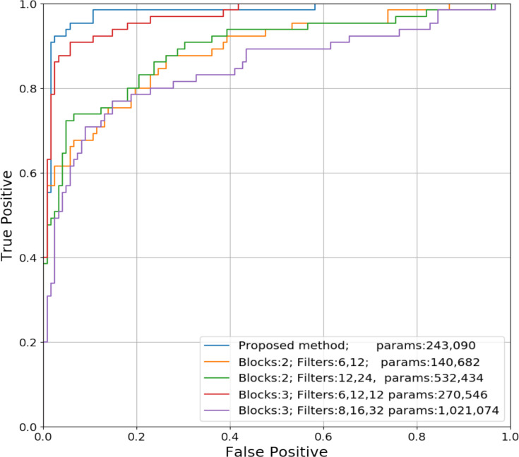
We compared the ROC curves of different Densely Connected CNNs (Figure 4). We observed that the curve with second highest AUC has 270,546 parameters, which is similar to that of the best performing DenseCNN model with 243,090 parameters. This further demonstrated that the proposed model is robust and has a suitable structure based on current data. The most complex model has over one million parameters, resulting the lowest AUC and sensitivity (67.7%), but it has higher accuracy than model with 532,434 parameters. Therefore, overly complex models may perform poorly in different aspects. Our experiments revealed that a lighter model with advanced structure can outweigh complicated models. Models with more layers and parameters is not necessary.

Figure 4. ROC curves of Densely Connected CNNs with different number of Dense Blocks and filters.

2.9. 4.3. Features visualization of DenseCNN

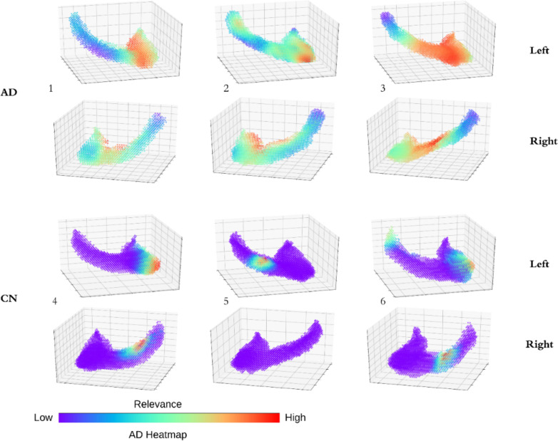
Deep learning methods are often criticized as Black Box, which is a major drawback for clinical applications. We illustrated the features related to AD prediction and provided visual information in an AD relevance 3D heatmap of 3 AD hippocampus and 3 CN hippocampus (Figure 5). We first computed the gradients from the output of the last Dense Block for a given hippocampus. We then averaged the gradients of all filters. The heatmaps are the overlays of the gradients and the input hippocampus. We can see that most parts in CN subjects has no relevance to AD. For example, the right hippocampus of the 5th subject has no relevance to those of AD subjects. Most parts in AD subject shows medium to high relevance. The high relevance areas are usually located in the lower head part of the hippocampus. The heatmap validated our results by visualizing the deep features of our model. Some CN hippocampus still has one or two small local areas highly related to AD, which may be explained as following: because of the shortcut connections in dense Block, the heatmap considers multiple convolutional layers at the same time. Consequently, both low- and high-level feature relevance are shown in the heatmap. Another possibility is that CN and AD subjects do share certain patterns, such as local textures and shapes, which may lead to some small but highly related areas in CN heatmaps. Our analysis of the relevance heatmap also showed the limitations of traditional shape and textured based methods duo to shared patterns between AD and CN subjects, which may provide insights for future improvements.

Figure 5. AD relevance heatmap: AD subjects (1-3) and CN subjects (4-6).

2.10. 4.4. Error analysis

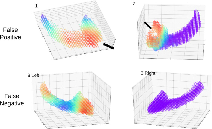
Three examples of misclassified subjects are shown in Figure 6. Example 1 and 2 are false positive (CN being misclassified as AD) and example 3 is false negative (AD being misclassified as CN). The false positives may be caused by missing voxels as shown in the first example and by a hole as shown in the second example (Figure 2). Only one side of the hippocampus is shown, because the other side has no observable missing voxels. Though we conducted quality control as mentioned in section 2.2 by manually viewing slices of segments., it is difficult to detect all missing parts in 3D plots as they can be observed only from a certain perspective. Minor differences between ground truth hippocampus and segmentation results do affect the performance of the model, as we can see that the voxel missing areas have high relevance to AD due to the fact that AD hippocampus may have concaves due to atrophy, which look similar to the pattens of the missing parts and holes. Unlike regular AD subjects who have relevance on both sides of hippocampus , the false negative (example 3 in Figure 6) has only left hippocampus showing some relevance to AD and the right showed no relevance at all. Consequently, the model misclassified example 3 as CN subject. These misclassified examples further demonstrated that AD is highly heterogeneous and the brain images varies among different AD patients.

Figure 6. 3 misclassified examples. Arrows indicating missing voxels in the hippocampus.

Discussion

In this study, we proposed a densely connected 3D-CNN model (DenseCNN) to classify AD and CN based on hippocampus imaging data from the ADNI database. DenseCNN achieved an overall best performance as compared to several state-of-art CNN methods. The following four reasons that may contributed to the high performance of DenseCNN: 1) advanced densely connected CNN architectures; 2) better hippocampus segmentation tools combined with manual curation; 3) more training data than previous method; 4) appropriate numbers of Dense Blocks and filters. Given the problem of limited data in biomedical domains, we focused on developing light models with fewer parameters. Compared to previous CNN models (e.g., Resnet¹⁶ and multi-model CNN¹⁷) with over 1 million parameters, Dense CNN has 243,090 trainable parameters. During our experiment, we found light models often outperformed more complex models.

Our study has a few limitations. First the quality of hippocampus segmentation is not perfect, which affected the overall performance as shown in our error analysis. Better segmentation tools, in the future, can further increase the performance of hippocamps based analysis method. Second, though our dataset consists of 326 AD subjects and 607 control normal (CN) subjects from the ADNI database, it still may not be large enough to train a CNN model with good generality. Third, we trained and tested DenseCNN using data from ADNI database. It will be important to test the model using data from other independent resources. Fourth, our current DenseCNN was trained based on hippocampus. Image features from other parts of the brains, for example total brain MRI, may further improve the oval performance. Fifth, incorporating non-imaging features such as patient genetics, genomics and demographics may further improve the performance. Finally, this study focused on classifying AD from CN, which is an easier problem than classifying subjects into AD, MCI and CN. Most MCI and AD cases have brain atrophy and share similar imaging features. Classifying AD and MCI via MRI is often more challenging and will require features other than imaging features.

Conclusion

In this paper, we developed a densely connected 3D-CNN model DenseCNN and compared it with several state-of-art 3D CNN methods. We demonstrated that DenseCNN has better or comparable performance while it is light, has significantly fewer number of parameters and is efficient to train. In summary, DenseCNN has potential as a robust, high performance and efficient diagnostic tools for AD classification.

Figures & Table

Figure 1. normal segment; wrong sections of brain; segmentations have noticeable missing voxels.

References

- 1.Alzheimer’s Association Alzheimer’s disease facts and figures. Alzheimer’s & Dementia. 2014 Mar 1;10(2):e47–92. doi: 10.1016/j.jalz.2014.02.001. 2014. [DOI] [PubMed] [Google Scholar]
- 2.Chugani HT, Phelps ME, Mazziotta JC. Positron emission tomography study of human brain functional development. Annals of neurology. 1987 Oct;22(4):487–97. doi: 10.1002/ana.410220408. [DOI] [PubMed] [Google Scholar]
- 3.Shaw LM, Vanderstichele H, Knapik-Czajka M, Clark CM, Aisen PS, Petersen RC, et al. Cerebrospinal fluid biomarker signature in Alzheimer’s disease neuroimaging initiative subjects. Annals of neurology. 2009 Apr;65(4):403–13. doi: 10.1002/ana.21610. [DOI] [PMC free article] [PubMed] [Google Scholar]
- 4.Jack CR, Jr, Bernstein MA, Fox NC, Thompson P, Alexander G, Harvey D, et al. The Alzheimer’s disease neuroimaging initiative (ADNI): MRI methods. Journal of Magnetic Resonance Imaging: An Official Journal of the International Society for Magnetic Resonance in Medicine. 2008 Apr;27(4):685–91. doi: 10.1002/jmri.21049. [DOI] [PMC free article] [PubMed] [Google Scholar]
- 5.Schuff N, Woerner N, Boreta L, Kornfield T, Shaw LM, Trojanowski JQ, et al. MRI of hippocampal volume loss in early Alzheimer’s disease in relation to ApoE genotype and biomarkers. Brain. 2009 Apr 1;132(4):1067–77. doi: 10.1093/brain/awp007. [DOI] [PMC free article] [PubMed] [Google Scholar]
- 6.Bron EE, Smits M, Van Der Flier WM, Vrenken H, Barkhof F, Scheltens P, et al. Standardized evaluation of algorithms for computer-aided diagnosis of dementia based on structural MRI: the CADDementia challenge. NeuroImage. 2015 May 1;111:562–79. doi: 10.1016/j.neuroimage.2015.01.048. [DOI] [PMC free article] [PubMed] [Google Scholar]
- 7.Hansson O, Seibyl J, Stomrud E, Zetterberg H, Trojanowski JQ, Bittner T, et al. CSF biomarkers of Alzheimer’s disease concord with amyloid-ß PET and predict clinical progression: A study of fully automated immunoassays in BioFINDER and ADNI cohorts. Alzheimer’s & Dementia. 2018 Nov 1;14(11):1470–81. doi: 10.1016/j.jalz.2018.01.010. [DOI] [PMC free article] [PubMed] [Google Scholar]
- 8.Ronneberger O, Fischer P, Brox T. Conference on Medical image computing and computer-assisted intervention. pp. 234-241. Vol. 5. Springer, Cham.; 2015. Oct, U-net: Convolutional networks for biomedical image segmentation. InInternational. [Google Scholar]
- 9.Ardila D, Kiraly AP, Bharadwaj S, Choi B, Reicher JJ, Peng L, et al. End-to-end lung cancer screening with three-dimensional deep learning on low-dose chest computed tomography. Nature medicine. 2019 Jun;25(6):954–61. doi: 10.1038/s41591-019-0447-x. [DOI] [PubMed] [Google Scholar]
- 10.Hosseini-Asl E, Keynton R, El-Baz A. In2016 IEEE International Conference on Image Processing (ICIP) IEEE; 2016. Sep 25, Alzheimer’s disease diagnostics by adaptation of 3D convolutional network; pp. 126–130. [Google Scholar]
- 11.Krizhevsky A, Sutskever I, Hinton GE. Imagenet classification with deep convolutional neural networks. InAdvances in neural information processing systems. 2012:1097–1105. [Google Scholar]
- 12.He K, Zhang X, Ren S, Sun J. Deep residual learning for image recognition. InProceedings of the IEEE conference on computer vision and pattern recognition. 2016:770–778. [Google Scholar]
- 13.Huang G, Liu Z, Van Der Maaten L, Weinberger KQ. Densely connected convolutional networks. InProceedings of the IEEE conference on computer vision and pattern recognition. 2017:4700–4708. [Google Scholar]
- 14.Ahmed OB, Benois-Pineau J, Allard M, Amar CB, Catheline G, Alzheimer’s Disease Neuroimaging Initiative. Classification of Alzheimer’s disease subjects from MRI using hippocampal visual features. Multimedia Tools and Applications. 2015 Feb 1;74(4):1249–66. [Google Scholar]
- 15.Cui R, Liu M. InTenth International Conference on Digital Image Processing (ICDIP 2018) Vol. 10806. International Society for Optics and Photonics; 2018. Aug 9, Hippocampus analysis based on 3D CNN for Alzheimer’s disease diagnosis; p. 108065O. [Google Scholar]
- 16.Li H, Habes M, Wolk DA, Fan Y. Alzheimer’s Disease Neuroimaging Initiative. A deep learning model for early prediction of Alzheimer’s disease dementia based on hippocampal magnetic resonance imaging data. Alzheimer’s & Dementia. 2019 Aug 1;15(8):1059–70. doi: 10.1016/j.jalz.2019.02.007. [DOI] [PMC free article] [PubMed] [Google Scholar]
- 17.Liu M, Li F, Yan H, Wang K, Ma Y, Shen L, et al. A multi-model deep convolutional neural network for automatic hippocampus segmentation and classification in Alzheimer’s disease. NeuroImage. 2020 Mar 1;208:116459. doi: 10.1016/j.neuroimage.2019.116459. [DOI] [PubMed] [Google Scholar]
- 18.Goubran M, Ntiri EE, Akhavein H, Holmes M, Nestor S, Ramirez J, et al. Hippocampal segmentation for brains with extensive atrophy using three-dimensional convolutional neural networks. Human brain mapping. 2020 Feb 1;41(2):291–308. doi: 10.1002/hbm.24811. [DOI] [PMC free article] [PubMed] [Google Scholar]
- 19.Patro S, Sahu KK. Normalization: A preprocessing stage. arXiv preprint arXiv:1503.06462. 2015. Mar 19,
- 20.Deng J, Dong W, Socher R, Li LJ, Li K, Fei-Fei L. In2009 IEEE conference on computer vision and pattern recognition. Ieee; 2009. Jun 20, Imagenet: A large-scale hierarchical image database; pp. 248–255. [Google Scholar]
- 21.Azulay A, Weiss Y. Why do deep convolutional networks generalize so poorly to small image transformations? Journal of Machine Learning Research. 2019 Jan 1;20(184):1–25. [Google Scholar]
- 22.Ioffe S, Szegedy C. Batch normalization: Accelerating deep network training by reducing internal covariate shift. arXiv preprint arXiv:1502.03167. 2015. Feb 11,
- 23.Srivastava N, Hinton G, Krizhevsky A, Sutskever I, Salakhutdinov R. Dropout: a simple way to prevent neural networks from overfitting. The journal of machine learning research. 2014 Jan 1;15(1):1929–58. [Google Scholar]
- 24.Ellis KA, Bush AI, Darby D, De Fazio D, Foster J, Hudson P. The Australian Imaging, Biomarkers and Lifestyle (AIBL) study of aging: methodology and baseline characteristics of 1112 individuals recruited for a longitudinal study of Alzheimer’s disease. International psychogeriatrics. 2009 Aug;21(4):672–87. doi: 10.1017/S1041610209009405. [DOI] [PubMed] [Google Scholar]