Building an Automated Orofacial Pain, Headache and Temporomandibular Disorder Diagnosis System

Abstract

Physicians collect data in patient encounters that they use to diagnose patients. This process can fail if the needed data is not collected or if physicians fail to interpret the data. Previous work in orofacial pain (OFP) has automated diagnosis from encounter notes and pre-encounter diagnoses questionnaires, however they do not address how variables are selected and how to scale the number of diagnoses. With a domain expert we extract a dataset of 451 cases from patient notes. We examine the performance of various machine learning (ML) approaches and compare with a simplified model that captures the diagnostic process followed by the expert. Our experiments show that the methods are adequate to making data-driven diagnoses predictions for 5 diagnoses and we discuss the lessons learned to scale the number of diagnoses and cases as to allow for an actual implementation in an OFP clinic.

1. Introduction

Diagnoses are one of the decisions physicians routinely make when encountering patients. Prior to an encounter with the physician, patients complete pre-encounter questionnaires with information on their medical history and a review of systems. To make decisions, physicians examine the answers provided in the questionnaires and any other available ancillary information, e.g., radiographic images or notes from a previous encounter as depicted in Figure 1. Physicians then make hypotheses on possible diagnoses and collect additional information asking questions or examining the patient, or prescribing tests to corroborate their hypothesis. This process requires both domain knowledge and expertise to avoid misdiagnosis. Expert physicians are more likely to carry out the process efficiently, e.g., without prescribing unnecessary tests, and they will converge quickly to make the correct decisions. To diagnose correctly, expert clinicians learn and retain a relatively large list of variables that define a wide variety of diagnoses. This is an imperfect process and failure to collect the needed data or failure to recognize the meaning of the collected data is not uncommon. In addition, novice physicians, e.g., physicians in training and non specialists, are at greater risk of making inefficient and/or incorrect decisions and these risks increase with uncommon diseases¹. Moreover, novice physicians either lack the necessary diagnostic and note taking skills, or generic interview practice fails to capture the discriminative features for specific diagnoses. The notes taken by novices may not contain the information needed for making the correct diagnoses or if the information is present it is not understood.

Figure 1:

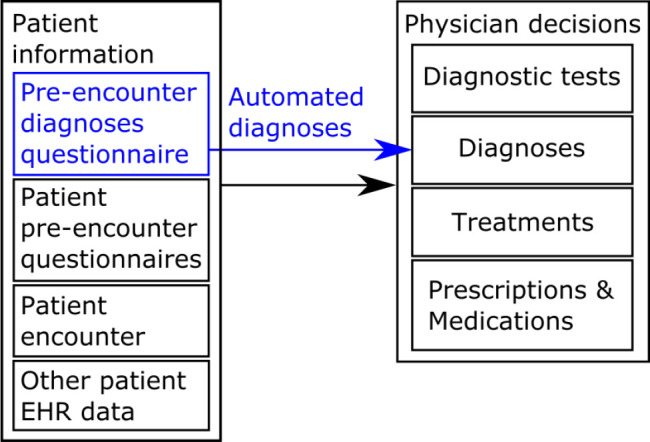
Clinical decision making process following patient encounters, and diagnoses automation using a patient filled pre-encounter diagnoses questionnaire (shown in blue).

One practical application of the predictions is to present clinicians with a set of diagnosis that they can validate or reject during a patient encounter. This could be achieved creating a patient facing questionnaire that will become a useful diagnostic adjunct. This would allow faster diagnosis times with potentially fewer misdiagnoses as long as the system performs equally or better than a typical clinician. In particular we believe that for clinicians in training automated diagnoses would be extremely valuable and that is our primary driving motivation with this work, since the system uses features (signs and symptoms) to narrow the number of possible conditions or diagnoses under consideration. A secondary clinical end point of the system would be to allow triaging incoming patients which would increase efficiency at a clinic and lower the burden on clinical resources, as long as the accuracy is sufficient compared to the information gathering process and decision making that would be needed. Furthermore ML approaches in these applications will allow us to select the most relevant features to use making the predictions, e.g., as a pedagogical tool for clinicians in training or as a set of features to focus the patient encounter on.

In this paper we are interested in the feasibility of automating the diagnosis of patients attending an orofacial pain (OFP) clinic who present with a variety of pain, headache and temporomandibular disorders. For this we want to augment the patient information of Figure 1 with a pre-encounter diagnoses questionnaire that is scored automatically. Most related work aimed at making OFP diagnostic prediction is on relatively small datasets and considers few diag-noses. These works either rely on patient notes which may fail because the discriminative variables are not recorded, or validated questionnaires that are prototyped based on expert opinion and which may omit other important variables and do not scale to the set of diagnoses that are needed for practical use in an OFP clinic. Therefore, our focus is on the process of generating data-driven patient questionnaires built on existing questionnaires and interview notes and that can be used to automate the diagnoses of orofacial pain disorders. For this we worked with an OFP expert at an OFP specialty clinic to build a suitable dataset and identify the relevant variables from recorded case notes. Our immediate goal is to examine the feasibility of automating and scaling the diagnosis process using supervised learning. While building the dataset we captured the expert thought process into a simplified expert model that we formalized and dubbed the High Frequency Value (HFV) model. We report on the performance of machine learning (ML) approaches and the simplified expert model and discuss the lessons learned on how to scale the number of diagnoses. While this work focuses on the automated diagnoses for OFP it is also of interest to other medical applications where pre-encounter questionnaires can be administered. The model predictions have in fact the potential to help physicians improve clinical outcomes by minimizing misdiagnoses through more efficient patient interviews with improved note taking.

The remainder of the paper is organized as follows: in Section 2 we discuss the related work. The dataset is presented in Section 3, Section 4 presents the methods used to create and validate the dataset. Results are presented in Section 5. Finally, in Section 6 we conclude the paper.

2. Related Work

Patient questionnaires are a prime source of information to physicians and this is especially so in a pain clinic. Some medical questionnaires are statistically validated for a target population. The PROMIS^®Patient-Reported Outcomes Measurement Information System² and consists of a set of person-centered measures that evaluates and monitors physical, mental, and social health in adults and children, can be used with the general population and with individuals living with chronic conditions. While PROMIS^®scores have been used to improve performance status assessment in cancer medicine³ and to predict postoperative outcomes⁴ their use to achieve an automated diagnosis remains limited. PROMIS short forms⁵ is an example of statistical questionnaires approach to select a small set of questions that are best understood and most predictive and remain a clinical standard. Statistically validated questionnaires such as PROMIS^®quantify the severity of a given outcome and cannot be applied to making multiple decisions such as diverging diagnoses.

With the increased use and availability of electronic health record (EHR) data, machine learning (ML) approaches have been used extensively for making data-driven clinical predictions^6,7. EHR data may include, patient interview notes, medical history, physical examination findings, imaging and laboratory test results. Several studies have used ML for clinical predictions, e.g., for symptom severity in mental care⁸, to diagnose common headaches⁹ and predict fertility¹⁰.

This work relies on traditional ML approaches (e.g., logistic regression, decision trees, support vector machine) that are known to perform well on smaller datasets.

Specifically, in the area of orofacial pain, narrative notes where used to diagnose four types of headaches⁹ from a set of 190 patients achieving accuracy levels greater than 90% concluding that if the data is sufficiently robust and the classification targets are sufficiently distinct, ML methods can provide a level of accuracy acceptable for use in clinical applications.

Several studies developed models to diagnose OFP from patient pre-interview questionnaires. McCartney et al. developed used a Neural Network (NN) to diagnose facial pain syndromes from patient’s self-assessment responses¹¹. Limonadi et al. used NN on a set of 143 patients to diagnose facial pain syndromes from a questionnaire with 18 binomial (yes/no) questions, obtaining good results on some of the 7 diagnoses that were considered¹². In other clinical applications, where large datasets are available, NN approaches have been shown to be successful, e.g., to predict optimal treatment strategies¹³. While these works realize the potential for pre-encounter diagnostic questionnaires they do not explore the process of selecting discriminative variables and how to scale beyond a limited set of diagnoses.

In this paper we specifically focus on using traditional supervised machine learning approaches as we build an OFP dataset for evaluation. The dataset we create is described in Section 3. Section 4 provides details on how we used a high frequency variable (HFV) algorithm to build the dataset and Section 5 presents the evaluation setup and results.

3. Dataset

The diagram of Figure 2 shows the process our OFP expert used to generate the OFP dataset that was ultimately used in the experiments of Section 5. To create the dataset, experts reviewed existing electronic patient notes, and for each case, extracted a set of features considered pertinent to the diagnoses based on domain knowledge and experience with the relevant diagnoses. Specifically, the expert, co-author Clark, initially bootstrapped the dataset process with 50 cases by identifying based on experience important variables and attempting to classify with a simple heuristic based on the features present. In parallel, to validate these 50 cases we have applied ML algorithms by training and testing on the same full set. This in turn has lead to identifying errors (such as missed relevant variables) and variables not present in the dataset which is typical in cases that get misclassified. We then iterated over this process expanding the dataset while formalizing the clinician expertise into the HFV model. A second expert, co-author Vistoso, independently extracted the features from the narrative notes and patient questionnaires and re-conciliated the feature set values over the entire dataset development process. Finally, we applied ML on the complete 451 cases dataset generating performance results including confusion matrices and examined cases that were misclassified leading to finding and correcting few more errors in the dataset, the majority of which resulted from typos in the spreadsheet that was used to create the dataset.

Figure 2:

Conceptual model used to generate and model the OFP dataset. Blue segments show how existing note taking protocols can be extended to include features used to improve the model performance. Ultimately, we aim at building models using information gathered through dynamic questionnaires.

The resulting dataset is formatted in the form of a dataframe¹⁴ as a table of rows, where each row corresponds to a case with features and labeled diagnoses. Variables were extracted from the patient interview encounter notes as filled by the physician and from the Medical History and Review of Systems questionnaires as filled by the patient. Notes taken by the physician include patient interview notes and selected examination variables. For our dataset this work was carried out manually, however applying natural language processing techniques to notes, that are usually captured as unstructured text, might allow us to automate this step. Throughout, we have tried to capture the expert thought process and found it to include the following steps for each case: (1) identify and reconfigure relevant diagnoses that could be achieved from patient input, (2) identify based on experience, the relevant variables that can be extracted from the notes, (3) wherever possible, make the extracted variables dichotomous (e.g., 1 if present and 0 if absent), (4) verify which variables are most prevalent (e.g., highest frequency) in all the cases where a given diagnosis occurs and (5) when a sufficient number of cases is available, classify the cases based on a similarity metric relating to the relative frequency of variables and diagnoses. To better capture this process and validate that it is sufficient for creating a robust dataset, we have implemented a simplified algorithm that proceeds according to steps 1-5 above. We have named the resulting algorithm the high frequency variable (HFV) algorithm and describe it in details in Section 4. The expert incrementally and iteratively built the final dataset by working in a spreadsheet and using the HFV algorithm for validation using the HFV computations described in Section 4. Our final dataset consisted of 451 cases: age range from 8 to 93, mean age is 43.4 years and age standard deviation is 21.4, with 320 females (71%) and 131 males (29%). We have considered 141 variables of which 138 are dichotomous, and 3 are continuous: age, pain severity on a discrete scale [0, 10], and max mouth opening in millimeters. The features include 6 variables that were used to quantize the continuous variables: age under 35, age over 59, pain severity lower or equal to 6, pain severity greater or equal to 8, and opening less or equal to 35 mm. We have limited our experiments in Section 5 to the 5 diagnoses presented in Table 1 for which the dataset has a sufficient number of positive samples. In the remainder of the paper we will refer to these 5 diagnoses as d1, d3, d4, d5 and d7 as show in Table 1. Each case in the dataset can have any or all of the diagnoses considered. Figure 2 shows the case counts for all possible combinations of the diagnoses considered, with the other category corresponding to cases that have other diagnoses than the 5 considered.

Table 1:

OFP diagnoses included in the experiment

	Diagnosis description	Freq.	% Rel. Freq.
d1	Internal derangement (DDWR) / Internal derangement (eDDNR)	169	37.47
d3	Masticatory or Cervical Myalgia/ Myofascial Pain	282	62.53
d4	Arthromyalgia Combo / Capsulitis	198	43.90
d5	TMJ Osteoarthritis / Rheumatoid Arthritis	83	18.40
d7	Chronic Trigeminal Neuropathy / Neuritis (not BMS)	63	13.97

4. Methods

We represent the set of questionnaire answers as a data vector of features X = [X₁, … , X_N] of size N, and formalize the diagnostic problem as a classification task that takes as input a vector X and outputs a label y for each possible diagnosis with y = [y₁, … , y_M] of size M. In the formulation of the HFV algorithm we restrict vectors X and y to contain binary values encoded as 0 and 1, i.e., X_i , y_i ∈ 0, 1 where 0 and 1 correspond to a value that is absent or present respectively. We assume K samples are available for training. In the following we describe the procedure for scoring a set of M diagnoses y with our HFV approach.

HFV Algorithm. Let f_ij be the relative frequency of feature i and label (i.e., diagnosis) j. We compute f_ij over the K training samples by counting the number of times the value of the feature corresponds to a positive label, i.e., feature value and diagnosis have a value of 1, and normalize by the count of samples with a positive label:

$$f_{ij}=\frac{{\displaystyle \sum {}_{k=1}^K}{X}_{ik}{y}_{jk}}{{\displaystyle \sum {}_{k=1}^K}{y}_{jk}{y}_{jk}}$$

We defined matrix of high frequency variables h of size M × N where h_ij is 1 if the relative frequency f_ij of feature i and label j is above a fixed threshold T_HF and 0 otherwise, i.e. h_ij = δ_T (f_ij), where the function δ_T = 1 if f_ij ≥ T_HF and δ_T = 0 otherwise. We then define the vector r_i of size N as the count of HFV for feature i:

$$r_i={\displaystyle \sum _{j=1}^M{h}_{ij}}$$

, and a weight vector w = [w₁, … , w_N] of size N with components $w_i=\frac{M}{r_i}$ if $r_i\ne 0$ and w_i = 0 otherwise. With W the diagonal matrix of w, we define the weighted matrix H of size M × N as H = hW. For a given input sample vector X = [x₁, … , x_N] the score vector s = [s₁, … , s_M] is given by s = HX. The ROC curve¹⁵ is used to determine the optimal score threshold to classify. Finally, we can estimate the confidence of label j as:

$$c_j=\frac{s_j}{{\displaystyle {\sum }_{i=1}^N{w}_i}}$$

5. Experiments

For developing the dataset, we initially implemented the HFV method of Section 4 in a spreadsheet and subsequently in python¹⁶ in order to compare with other ML approaches. We used Scikit-learn¹⁷ to implement and evaluate HFV, Random Forest, SVM, Logit and k-NN classifiers. Due to the relatively small size we only use ML approaches.

Classification Methods. Several classification algorithms were used to categorize the diagnoses. Extracted dichotomous features were labeled using a binary value (1 or 0 depending on whether the feature is present or absent) and used for training. We evaluate using HFV, Random Forest, SVM, Logit (Logistic Regression), and k-NN classifiers using scikit-learn¹⁷. Random Forest can be trained to classify labels one at the time or to classify all labels at once, i.e., multilabel classification, hence we examined both modalities. Combining classifiers was shown to improve performance¹⁸. We therefore report performance measurements for different combinations of classifiers using two ensemble methods: Average of Probabilities¹⁹ and Majority Voting²⁰. The Average of Probabilities fusion method returns the mean value of probabilities of multiple classifiers. The Majority Voting returns the class which gets the most votes among multiple classifiers.

Parameter Tuning. Classification parameters were adjusted for best results. The HFV method used T_HF = 0.67, i.e., we consider that a feature is a high value feature if it is positive for a positive diagnosis at least 2/3 of the time. Random Forest classifiers used 100 estimators (number of trees). SVM classifier used a slack variable cost C = 1 with radial basis function kernel, and continuous variables were scaled using min-max scaling. Logit used a stochastic average gradient SAG solver²¹. We used a K-fold cross validation with K = 5 and reported performance averaged over the folds.

Results. Table 2 presents, for the five diagnoses listed in Table 1, the classification results of seven classifiers: HFV multilabel, Random Forest multilabel, Random Forest, Logit, SVM, and k-NN. To make a fair comparison with the HFV method that is not designed to deal with continuous variables, we have replaced the continuous variables with corresponding quantized features as described in Section 3. Overall the accuracy ranges from 75.60% to 96.89%, precision ranges from 52.40% to 97.38%, recall ranges from 46.27% to 98.21%, and F-1 score ranges from 0.56 to 0.96. Classification accuracy rates per diagnosis are in decreasing order: d1, d5, d3, d7 and d4. Best accuracy: d1 (RFml / SVM 96.89%), d3 (SVM 93.34%), d4 (SVM 89.56%), d5 (RF 96.22%) and d7 (k-NN 91.57%). Compared to the best classifiers results, HFV achieves lower accuracy rates: d1 (-1.29%), d3 (-11.31%), d4 (-7.54%), d5 (-0.44%) and d7 (-5.52%). Overall HFV accuracy ranges from 82.02% to 95.78%, which seems to indicate that HFV was capable of capturing the expert decision making thought process and support the database building process. However, as HFV was used to build and test the dataset we note that the database might be biased towards the HFV method.

Table 2:

Classification performance for diagnoses d1, d3, d4, d5 and d7. RF: random forest, ml: multilabel, A: accuracy, P: precision, R: recall, and F1: F1-score. Best performance is shown in bold.

d1		A (%)	P (%)	R (%)	F1
	HFV ml	95.56	94.15	93.18	0.94
	RF ml	96.89	96.24	94.47	0.95
	RF	96.22	95.02	93.83	0.94
	Logit	96.00	95.93	92.76	0.94
	SVM	96.89	97.38	93.83	0.95
k-NN	92.23	86.21	93.62	0.89
d3	HFV ml	84.03	91.17	82.24	0.85
	RF ml	93.79	93.36	97.14	0.95
	RF	93.57	93.80	96.32	0.95
	Logit	93.34	93.83	96.04	0.95
	SVM	95.34	94.95	98.21	0.96
k-NN	83.82	87.40	86.49	0.86
d4	HFV ml	82.02	77.58	86.52	0.81
	RF ml	88.90	86.32	92.03	0.88
	RF	87.79	85.95	90.65	0.87
	Logit	88.91	86.31	91.52	0.88
	SVM	89.56	85.20	96.22	0.89
k-NN	75.60	69.56	82.32	0.75
d5	HFV ml	95.78	89.32	89.42	0.89
	RF ml	95.78	93.44	85.14	0.89
	RF	96.22	93.57	87.43	0.90
	Logit	88.91	86.31	91.52	0.88
	SVM	95.34	92.46	83.32	0.87
k-NN	92.46	90.18	65.65	0.76
d7	HFV ml	86.05	52.40	81.96	0.62
	RF ml	90.24	73.00	49.46	0.58
	RF	90.90	75.05	52.99	0.60
	Logit	90.02	67.50	54.99	0.60
	SVM	90.24	73.10	46.27	0.56
k-NN	91.57	77.22	53.56	0.63

We speculate that the lower HFV accuracy (82.02%) for the arthralgia diagnosis d4 was because this diagnosis had almost the same set of features as diagnosis d3 (myalgia), making it very hard to distinguish. Additional features are needed in the narrative note to better make this distinction or if they cannot be separated, highly overlapping diagnoses might need to be combined. Diagnoses d7 (trigeminal neuropathic pain) was also more difficult to predict and exhibited the lowest precision and accuracy levels. This diagnoses had the smallest relative positive diagnosis frequency (13.97%). However, for diagnosis d7, we hypothesize that a critical defining variable (e.g., focal allodynia, which is pain with non-painful stimulation) was not consistently captured in the narrative note but was needed for this diagnosis. Careful examination of feature data and expertise in the domain, allows speculation regarding which variables are missing. With this knowledge, we will need to amend the note-taking protocol and once new cases are collected to assess our hypotheses.

Table 3 presents classification results for top single classifiers of Table 2 and the three top combinations of classifiers considering the continuous variables (age, pain severity and max mouth opening) and excluding the related quantized features that were introduced to support the comparison with HFV in the results of Table 2. Classifier considered: Random Forest (RF), Random Forest multiclass (RF ml), Logit and SVM, Classifier combinations considered: Random Forest and SVM (RS), SVM and k-NN (Sk), Random Forest and SVM and Logit (RSL), Random Forest and Logit (RL). We label the combinations as mv for majority vote and ap for average of probabilities.

Table 3:

Single and combinations of classifiers performance (continuous variables included). RF: random forest, ml: multilabel, RL: Random Forest and Logit, RS: Random Forest and SVM, Sk: SVM and k-NN, RSL: Random Forest, SVM and Logit, ap: average of probabilities, mv: majority voting, A: accuracy, P: precision, R: recall, and F1: F1-score. Best performance is shown in bold.

d1		A (%)	P (%)	R (%)	F1
	RF ml	96.45	97.38	92.76	0.95
	Logit	95.78	95.93	92.35	0.94
	SVM	97.11	98.04	93.83	0.96
	RS mv	97.11	98.04	93.83	0.96
	Sk mv	95.79	98.46	90.13	0.94
RSL mv	96.89	98.04	93.18	0.95
d3	RF ml	94.01	94.08	96.70	0.95
	Logit	93.57	93.83	96.44	0.95
	SVM	95.34	94.95	98.21	0.96
	RL ap	93.57	93.83	96.44	0.95
	RS mv	93.79	94.52	96.02	0.95
Sk mv	93.35	94.45	95.28	0.95
d4	RF ml	89.57	86.88	93.15	0.89
	Logit	89.57	86.98	92.65	0.89
	SVM	89.78	85.21	96.75	0.90
	RL ap	88.68	85.88	93.15	0.88
	RS mv	88.91	87.92	89.40	0.88
RSL mv	89.13	87.77	89.72	0.88
d5	RF ml	95.12	93.12	81.10	0.87
	Logit	95.34	91.46	84.44	0.87
	SVM	95.34	92.46	83.32	0.87
	RL ap	95.56	92.63	84.44	0.88
	RS mv	95.12	93.29	81.04	0.87
Sk mv	95.34	93.44	82.15	0.87
d7	RF ml	90.23	68.49	49.35	0.56
	Logit	90.02	66.61	56.99	0.61
	SVM	90.68	75.60	49.52	0.59
	RL ap	90.90	72.17	59.10	0.64
	RS mv	90.68	79.38	47.46	0.58
Sk mv	90.68	76.78	48.71	0.58

Overall the accuracy ranges from 88.68% to 97.11%, precision ranges from 66.61% to 98.46%, recall ranges from 47.46% to 98.21%, and F-1 score ranges from 0.56 to 0.96. Similar to the results of Table 2, classification accuracy rates per diagnosis are in decreasing order: d1, d5, d3, d7 and d4. Best accuracy: d1 (RS mv / SVM 96.89%), d3 (RF ml 93.34%), d4 (SVM 89.56%), d5 (RL ap 95.56%) and d7 (RL ap 90.90%).

Tables 4 and 5 present an example for a combinations of factors intervening in a typical single label Random Forest prediction ordered by Gini coefficient. For the set of diagnoses considered, the topmost feature are all different, however some of the secondary and tertiary features appear in several diagnoses, e.g., age. Note that several features are the result of a physical examination; in a patient facing questionnaires these features could be reported by the patient as self examination. In general, features interpretability information can be used to assess the dataset and to inform physicians.

Table 4:

Top 3 features for Random Forest single label classifier ordered by Gini coefficient from most important (1) to least important (3) for diagnoses d1, d3, d4, d5 and d7.

	First most important	Second most important	Third most important
d1	exam tmj click (0.273)	tmjd clicking (0.147)	age (0.1)
d3	exam muscle tenderness (0.274)	extraoral jaw muscle (0.059)	age (0.058)
d4	exam tmj tenderness (0.24)	age (0.079)	exam muscle tenderness (0.062)
d5	exam tmj crunch (0.333)	tmjd crunching (0.16)	age (0.064)
d7	exam tooth pain problem (0.17)	cc tooth (0.09)	intraoral gingival (0.044)

Table 5:

Descriptions for the labels of Table 4. Labels prefixed with exam_ were extracted from patient encounter notes as confirmed by the clinician during the patient examination. TMJ refers to the temporomandibular joint.

Label	Description
age	subject age
cc tooth	chief complaint is problem with teeth or tooth
exam muscle tenderness	palpation tenderness in jaw or neck muscles
exam tmj click	auscultation shows click sound in TMJ on movement
exam tmj crunch	auscultation shows crunching in TMJ on movement
exam tmj tenderness	palpation tenderness in jaw joint
exam tooth pain problem	pain in the teeth confirmed by examination
extraoral jaw muscle	location of symptoms in jaw muscles
intraoral gingival	location of symptoms in gingival tissues
tmjd clicking	patient reports TMJ clicking
tmjd crunching	patient reports TMJ crunching

6. Conclusion

Automating the journey from data collection to diagnoses has the potential to improve standards of care by providing faster and reliable predictions. In addition predictions can inform physicians in training by relating important combinations of variables to potential diagnoses. For this end we propose in upcoming work to create and validate a pre-encounter patient questionnaire that can predict a variety of OFP diagnoses.

In this work, we examine how an OFP dataset can be created and explore the feasibility of automating OFP diagnoses with pre-encounter questionnaires. Working with an expert we have captured the expert’s thought process to look for the relevant variables and derived an algorithm to modeled this process, the HFV algorithm, that was implemented and used to iteratively and incrementally create an OFP dataset of 451 cases each containing 137 independent features. We report results of a comparative analysis of the HFV method with other machine learning models as a validation of the dataset creation process and best classification results obtained by using a combination of classifiers. These results show that the process used to define variables, forming the dataset is sound and the use of ML models to automate diagnoses is feasible. We understand that the HFV system was used in building the dataset and therefore has a bias, but it also validates the conceptual model clinicians use in patient interviews. Furthermore, the quality of the predictions seem to indicate that the process we use to generate the dataset (which questions are important to ask) is sound.

Any practical application of ML predictions will require addressing differential diagnoses and combination diagnoses. With this work we have shown that it is feasible to automate specific diagnosis if the needed features are present. In our future work we will examine how ML approaches and classifier metrics can be used to support both differential and combinatorial diagnoses by extending the number of cases and considering a wider set of OFP diagnoses. For this we plan to utilize natural language processing to extract the variables from the electronic patient notes. In addition we will update our note taking protocols to ensure that the variables that are discovered as important for the performance of the system are captured. We will seek to improve our algorithms once we scale the dataset to prove feasibility with additional OFP diagnoses. Finally, we will examine how to best create predictive patient questionnaires, e.g., how to formulate the questions so they can be best understood and answered easily and how to only ask the questions relevant to the diagnoses for the case at hand.

7. Acknowledgement

This work has been supported internally by Orofacial Pain and Oral Medicine Center at the Herman Ostrow School of Dentistry of USC. The opinions, findings, and conclusions or recommendations expressed in this material are those of the authors and do not necessarily reflect the views of the sponsors.

Figures & Table

Figure 3:

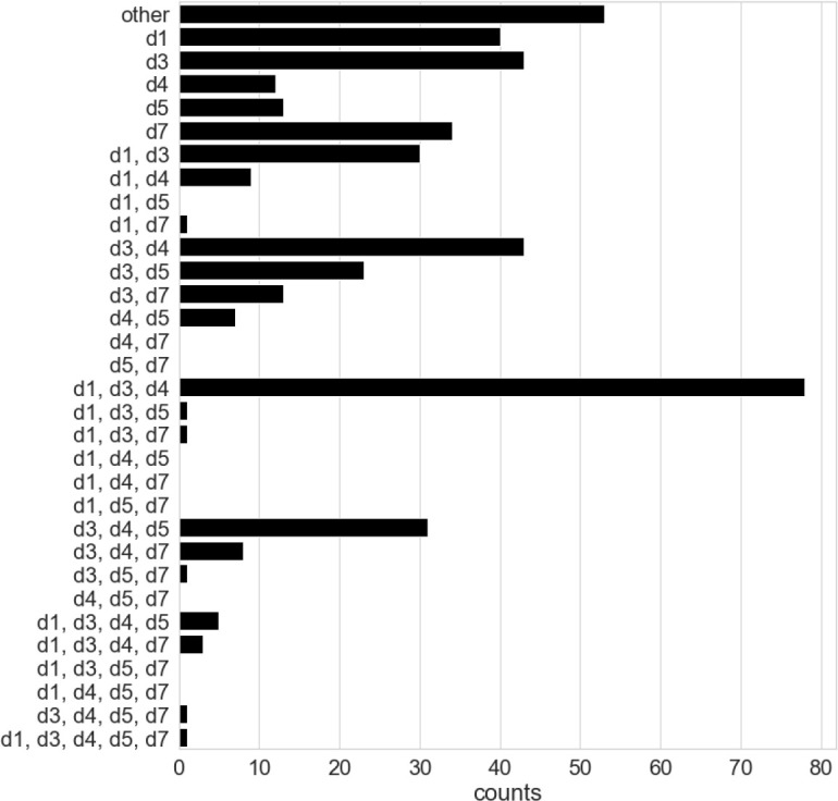
Dataset case counts by diagnoses combinations. “other” refers to diagnoses not considered in this study.

References

- 1.Hardeep Singh, Schiff Gordon D, Graber Mark L. Igho Onakpoya, and Matthew J Thompson. The global burden of diagnostic errors in primary care. BMJ Qual Saf. 2017;26(6):484–494. doi: 10.1136/bmjqs-2016-005401. [DOI] [PMC free article] [PubMed] [Google Scholar]
- 2.PROMISQR measurement system Url: http://www.healthmeasures.net/ Last accessed on 2020-03-17.
- 3.Broderick Joan E, Marcella May, Schwartz Joseph E, Ming Li, Aaron Mejia, Luciano Nocera, Anand Kolatkar, Ueno Naoto T, Sriram Yennu, Lee Jerry SH, et al. Patient reported outcomes can improve performance status assessment: a pilot study. Journal of patient-reported outcomes. 2019;3(1):41. doi: 10.1186/s41687-019-0136-z. [DOI] [PMC free article] [PubMed] [Google Scholar]
- 4.Anderson Michael R, Houck Jeff R, Saltzman Charles L, Man Hung, Florian Nickisch, Alexej Barg. Timothy Beals, and Judith F Baumhauer. Validation and generalizability of preoperative promis scores to predict postop- erative success in foot and ankle patients. Foot & ankle international. 2018;39(7):763–770. doi: 10.1177/1071100718765225. [DOI] [PubMed] [Google Scholar]
- 5.Lan Yu, Buysse Daniel J, Anne Germain, Moul Douglas E, Angela Stover, Dodds Nathan E. Kelly L Johnston, and Paul A Pilkonis. Development of short forms from the promisTM sleep disturbance and sleep-related impairment item banks. Behavioral sleep medicine. 2012;10(1):6–24. doi: 10.1080/15402002.2012.636266. [DOI] [PMC free article] [PubMed] [Google Scholar]
- 6.Jonathan H Chen, Steven M Asch. Machine learning and prediction in medicine—beyond the peak of inflated expectations. The New England journal of medicine. 2017;376(26):2507. doi: 10.1056/NEJMp1702071. [DOI] [PMC free article] [PubMed] [Google Scholar]
- 7.Wei-Hung Weng. Machine learning for clinical predictive analytics. arXiv preprint arXiv:1909.09246. 2019.
- 8.George Karystianis, Nevado Alejo J, Chi-Hun Kim, Azad Dehghan, Keane John A, Goran Nenadic. Auto- matic mining of symptom severity from psychiatric evaluation notes. International journal of methods in psychi- atric research. 2018;27(1):e1602. doi: 10.1002/mpr.1602. [DOI] [PMC free article] [PubMed] [Google Scholar]
- 9.Monire Khayamnia, Mohammadreza Yazdchi, Aghile Heidari, Mohsen Foroughipour. Diagnosis of common headaches using hybrid expert-based systems. Journal of medical signals and sensors. 2019;9(3):174. doi: 10.4103/jmss.JMSS_47_18. [DOI] [PMC free article] [PubMed] [Google Scholar]
- 10.Sahoo Anoop J, Yugal Kumar. Seminal quality prediction using data mining methods. Technology and Health Care. 2014;22(4):531–545. doi: 10.3233/THC-140816. [DOI] [PubMed] [Google Scholar]
- 11.Shirley McCartney. Markus Weltin, and Kim J Burchiel. Use of an artificial neural network for diagnosis of facial pain syndromes: an update. Stereotactic and functional neurosurgery. 2014;92(1):44–52. doi: 10.1159/000353188. [DOI] [PubMed] [Google Scholar]
- 12.Limonadi Farhad M. Shirley McCartney, and Kim J Burchiel. Design of an artificial neural network for diagnosis of facial pain syndromes. Stereotactic and functional neurosurgery. 2006;84(5-6):212–220. doi: 10.1159/000095167. [DOI] [PubMed] [Google Scholar]
- 13.Matthieu Komorowski, Celi Leo A, Omar Badawi. Anthony C Gordon, and A Aldo Faisal. The artificial intel- ligence clinician learns optimal treatment strategies for sepsis in intensive care. Nature medicine. 2018;24(11):1716–1720. doi: 10.1038/s41591-018-0213-5. [DOI] [PubMed] [Google Scholar]
- 14.Wes McKinney. Python for data analysis: Data wrangling with Pandas, NumPy, and IPython”. 2012. O’Reilly Media, Inc”. [Google Scholar]
- 15.Leo Breiman, Jerome Friedman, Charles J Stone, Richard A Olshen. Classification and regression trees. CRC press; 1984. [Google Scholar]
- 16.Python implementation of the hfv classifier Url: https://bitbucket.org/nocera/hfv-classifier. Last accessed on 2020-03-17.
- 17.Fabian Pedregosa, Gae¨l Varoquaux, Alexandre Gramfort, Vincent Michel, Bertrand Thirion, Olivier Grisel, Math- ieu Blondel, Peter Prettenhofer, Ron Weiss, Vincent Dubourg, et al. Scikit-learn: Machine learning in python. Journal of machine learning research. 2011;12(Oct):2825–2830. [Google Scholar]
- 18.Lior Rokach. Ensemble-based classifiers. Artificial Intelligence Review. 2010;33(1-2):1–39. [Google Scholar]
- 19.Robert PW Duin, David MJ Tax. Experiments with classifier combining rules; International Workshop on Multiple Classifier Systems; Springer. 2000. pp. 16–29. [Google Scholar]
- 20.Dymitr Ruta, Bogdan Gabrys. Classifier selection for majority voting. Information fusion. 2005;6(1):63–81. [Google Scholar]
- 21.Mark Schmidt, Nicolas Le Roux, Francis Bach. Minimizing finite sums with the stochastic average gradient. Mathematical Programming. 2017;162(1-2):83–112. [Google Scholar]