An electrophysiological megastudy of spoken word recognition

Abstract

This study used electrophysiological recordings to a large sample of spoken words to track the time-course of word frequency, phonological neighbourhood density, concreteness and stimulus duration effects in two experiments. Fifty subjects were presented more than a thousand spoken words during either a go/no go lexical decision task (Experiment 1) or a go/no go semantic categorisation task (Experiment 2) while EEG was collected. Linear mixed effects modelling was used to analyze the data. Effects of word frequency were found on the N400 and also as early as 100 ms in Experiment 1 but not Experiment 2. Phonological neighbourhood density produced an early effect around 250 ms and the typical N400 effect. Concreteness elicited effects in later epochs on the N400. Stimulus duration affected all epochs and its influence reflected changes in the timing of the ERP components. Overall the results support cascaded interactive models of spoken word recognition.

Introduction

Our ability to recognise spoken words is one of the most frequently used and important of our cognitive skills. So, it is perhaps somewhat surprising that there is much we still do not know about the underlying neuro-cognitive processes that are involved in mapping sound onto meaning. Though perceived as effortless, the ability to decode continuous, transient auditory information into a single word from tens of thousands of candidates within a fraction of a second involves a highly complex set of neuro-cognitive process. This task is further complicated by the fact that many words are acoustically quite similar to each other and that human speech is extremely variable due to both idiosyncratic speaker characteristics and phonological context which influences the acoustic properties of phonemes depending on neighbouring phonemes. Clearly, semantic and syntactic context have important roles in spoken language comprehension in real world contexts, but there is a general consensus that such higher-level processing is driven primarily by mechanisms operating at the level of individual words. Models of spoken word recognition generally agree that this involves multiple hierarchical levels, which begin operating on partial information that activates representations of multiple word candidates in parallel which then compete for recognition.

One approach to untangling the array of underlying mechanisms involved in word recognition is to examine the impact of various linguistic factors on this process. The bulk of the work using this approach has employed behavioural dependent variables such as reaction time, although these measures largely occur after the processes of interest and therefore do not directly reflect the brain activity of the underlying neuro-cognitive processes. Moreover, such behavioural measures are generally unitary, offering a limited perspective on the dynamic nature of word processing. This latter issue might be particularly important in the case of spoken language where words unfold over time. Because they continuously reflect information processing in real time, event-related brain potentials (ERPs) have proven to be an excellent choice for studying the temporal dynamics of spoken word processing. However, while many studies have used ERPs to track the time course of visual word recognition (e.g. Grainger & Holcomb, 2009; Hauk, Davis, Ford, Pulvermüller, & Marslen-Wilson, 2006), there are comparatively fewer studies of spoken word recognition (see Hagoort & Brown, 2000, for one example) and there are none that have looked at the influence of a wide array of linguistic variables. Here we report on a study in which fifty participants listened to over a thousand single spoken words while EEG was recorded.

Perhaps the most studied lexical variable in studies of word recognition is word frequency, which is typically measured as the number of occurrences of a word in a given corpus of written or spoken language. The basic finding, which has been widely replicated, is that listeners are more accurate and have faster reaction times to high frequency compared to low frequency words in a variety of tasks (see Rubenstein, Garfield, & Millikan, 1970, for an early demonstration, and Ferrand et al., 2017, for a recent megastudy). In spoken word recognition models, such word frequency effects can be accounted for in a number of ways. In activation models, higher frequency lexical units can have lower activation thresholds (Marslen-Wilson, 1990), higher resting states of activation (McClelland & Elman, 1986), stronger connections between units (Dahan, Magnuson, & Tanenhaus, 2001) or in a Bayesian modelling framework by assuming frequency effects reflect the higher prior probability for high frequency words (Norris & McQueen, 2008). Alternatively, models such as the Neighbourhood Activation Model (NAM) suggest that word frequency does not affect processing at a lexical level, but rather acts as a post-lexical decision bias (Luce & Pisoni, 1998). Of course, it is entirely possible that a complex variable such as word frequency exerts an influence on spoken word comprehension across multiple processing levels and that the pattern of its influence may be sensitive to the task demands placed on the listener.

In ERP research on visual word recognition, word frequency manipulations have been shown to modulate the amplitude of the N400 (e.g. Smith & Halgren, 1987) a component usually associated with lexico-semantic processing. Thus, larger N400s for lower frequency words may reflect the increased processing necessary to map lexical representations of lower frequency words onto their meanings (Kutas & Federmeier, 2011). Consistent with this view is the finding that word frequency effects on the N400 decline as other factors that facilitate word processing (e.g. context) increase (Van Petten & Kutas, 1990). In addition to the N400 there has been conflicting evidence that earlier ERP components (as early as the N1) also are sensitive to manipulations of word frequency, at least in the visual modality (e.g. Chen, Davis, Pulvermüller, & Hauk, 2015; Hauk et al., 2006; Sereno, Rayner, & Posner, 1998). In their ERP megastudy using the same stimuli and a similar experimental design to the current study (see below), Dufau, Grainger, Midgley, and Holcomb (2015) found a very small effect of word frequency emerging at posterior (occipital) sites between 200 and 300 ms, with the largest effects of frequency occurring on the N400.

Effects of word frequency on spoken word ERPs have also been reported. In one study Dufour, Brunelliere, and Frauenfelder (2013) found that low frequency spoken words produced a larger anterior positivity and posterior negativity at 350 ms compared to high frequency words. Similar to written words, they also found larger late N400 activity (550 to 650 ms) for low compared to high frequency spoken words. The lateness of the second effect (550 to 650 ms) could be consistent with a post-lexical locus of word frequency for spoken words, while the bipolar effect across the scalp at 350 ms might reflect a pre-recognition influence of word frequency.

Another variable that has been shown to influence spoken word processing is phonological neighbourhood density (PND). PND is a measure of the number of other words that are phonologically similar to a given word. Behaviourally, spoken words with dense neighbourhoods (i.e. words that share phonological characteristics with many other words) tend to be recognised more slowly and with less accuracy than words with fewer neighbours (Goldinger, Luce, & Pisoni, 1989). This pattern has been suggested to indicate the influence of interference or competition from the other similar words in a target word’s phonological neighbourhood (e.g. Vitevitch & Luce, 1999). This competition between similar sounding words is assumed by many models of spoken word recognition, however it is incorporated in different ways. In the Cohort model (Marslen-Wilson, 1987), words which share initial phonemes are co-activated and compete for recognition as more information becomes available. This predicts neighbourhood effects, but only among words which initially resemble each other (cohorts) and not with other sorts of phonological neighbours such as rhymes, which nevertheless have also been found to produce neighbourhood effects (e.g. Connine, Blasko, & Titone, 1993). The Neighbourhood Activation Model (NAM: Luce & Pisoni, 1998) provides a relatively simple and effective mathematical account of PND effects, although it does not incorporate the dynamic nature of speech (input that unfolds over time), and thus has difficulty explaining why cohorts produce more competition than rhymes (Allopenna, Magnuson, & Tanenhaus, 1998). Other models such as TRACE (McClelland & Elman, 1986) and Shortlist (Norris, 1994) better account for dynamic neighbourhood effects, though TRACE includes feed-back connections while Shortlist is only feed-forward. It should also be noted that facilitatory effects of PND have been found with the auditory lexical decision task (Ernestus & Cutler, 2015; Ferrand et al., 2017; Goh, Yap, Lau, Ng, & Tan, 2016), again suggesting that task demands might differentially alter the influence PND has on underlying mechanisms.

Effects of neighbourhood density have also been reported in ERP research. Most of this work has involved visual word recognition where words from large orthographic neighbourhoods (the visual equivalent of phonological neighbourhoods) have been shown to generate larger N400s than words from small orthographic neighbourhoods (e.g. Holcomb, Grainger, & O’rourke, 2002; Laszlo & Federmeier, 2011). This greater N400 to high density words is thought to reflect the additional activation of a target word’s neighbours (Holcomb et al., 2002). In their megastudy Dufau et al. (2015) found that orthographic neighbourhood effects were largely restricted to the early phase of the N400 window (300 to 400 ms). Two studies have used ERPs to examine PND effects in spoken word recognition. Dufour et al. (2013) found smaller early positivities (250–330 ms) and larger N400s to French words with more phonological neighbours. A second study in English (Hunter, 2013) found larger P2 amplitudes to words with more neighbours but did not report any effects on the N400.

Relative concreteness is another variable that has been shown to affect word recognition. Concrete words are responded to faster than abstract words in a variety of tasks (e.g. lexical decision; Goh et al., 2016; Whaley, 1978). This effect is usually explained by concrete words having greater semantic richness (Kieras, 1978), greater tendency to induce the use of mental imagery (Paivio, 1986), or some combination of both (Holcomb et at., 1999). In the visual domain, research with ERPs has identified two components which are both more negative to more concrete than abstract words; the N400 (Kounios & Holcomb, 1994) and a later component around 700 ms (West & Holcomb, 2000). While the effect of concreteness on the N400 is thought to reflect greater activation of lexical-semantic networks as mentioned above, the later effect at 700 ms is thought to represent a process related to mental imagery (West & Holcomb, 2000). In the visual megastudy by Dufau et al. (2015), concreteness effects paralleled those from previous ERP studies with larger late negativities for more concrete words starting around 300 ms and continuing on through the N400 epoch (Dufau et al., did not report effects beyond 500 ms). It is worth noting that in the case of concreteness, N400 amplitude seems to be negatively correlated with reaction time thus indicating a facilitative role, yet in the case of word frequency (and some, but not all neighbourhood effects), larger N400s are usually associated with longer reaction times, consistent with competition or more effortful processing. To date, we are unaware of any ERP studies that have manipulated concreteness with auditory words.

Another variable relevant to lexical processing is the length of words being comprehended. In the case of visual words the number of letters determines length. In the case of spoken words it is the temporal duration that is associated with length. And while these two indices are correlated (e.g. number of letters and numbers of phonemes), there is reason to predict that that the influence of these two indices of length might operate differently during word processing. In visual word recognition there is strong evidence of parallel letter processing within a single fixation (e.g. Grainger, 2008). However, because length for spoken words translates to the temporal domain and thus necessitates some degree of serial processing, the duration of a spoken word is likely to play a more important role during spoken word recognition than number of letters does in visual word recognition. In the case of spoken words, measures such as word duration, number of phonemes and uniqueness point are temporal variables that have been shown to influence word recognition. Although not as frequently examined, a few behavioural studies have looked for effects of spoken word duration (e.g. Pitt & Samuel, 2006; Strauss & Magnuson, 2008). In these studies duration has been suggested to have a somewhat counter intuitive effect on the dynamics of word processing. Although longer spoken words take longer to recognise, they also result in greater lexical activation presumably because of their having additional acoustic information to influence processing. In their auditory lexical decision megastudy, Ferrand et al. (2017) reported that stimulus duration was the variable that accounted for the most variance (46%, followed by word frequency at 4% of additional variance, with a strong positive correlation between stimulus duration and RT - see also Ernestus & Cutler, 2015; Goh et al., 2016).

In the ERP literature on word length, the number of letters in a visually presented word has been shown to influence ERPs both quite early as well as later during word processing. For example, Hauk and Pulvermüller (2004) reported that longer visual words produced increased activity as early as 80 ms while shorter words elicited greater negativity in epochs up to 400 ms. The Dufau et al. (2015) megastudy found effects of word length emerging at around 200 ms and continuing into later epochs. Longer words tended to produce more negative-going waves than shorter words at 200 ms, and during the N400 epoch shorter words produced greater negativities. Of course, one confound for such visual effects is that longer words also tend to be larger stimuli, and increases in the size of any stimulus tends to produce larger early ERP effects (e.g. Luck, 2005). To our knowledge no study has looked at ERPs to spoken words as a function of word duration. One prediction based on the results of Pitt and Samuel (2006) is that while the time-course of ERP effects might be delayed for longer words, it might also be the case that longer words generate larger N400s than shorter words due to their activation of additional phonemic information. Note this prediction is the opposite of what Dufau et al. reported for visual word length effects.

The current study

The purpose of the current study was to use ERPs to provide a better understanding of how the above variables (word frequency, phonological neighbourhood density, concreteness and duration) affect the temporal dynamics of spoken word recognition. In all previous auditory ERP studies, variables such as these have been factorially manipulated and measures of processing have been obtained. However, this approach, which is arguably arbitrary in terms of where boundaries are placed for categorising what is a continuous variable, may oversimplify, or take away from, the complexity and variability that is inherent in language. Recently, researchers have begun conducting “megastudies” which seek to better understand these complexities by gathering data with large samples of participants and items. This method has a number of advantages including reduced experimenter bias towards item selection and the ability to run more advanced types of analyses (see Balota, Yap, Hutchison, & Cortese, 2012 for a review of advantages). This has been fruitfully applied to study visual word recognition with behavioural data (e.g. Balota et al., 2007; Ferrand et al., 2017) and ERP data (e.g. Hauk et al., 2006; Laszlo & Federmeier, 2014).

One such ERP study conducted by Dufau et al. (2015) presented over 1000 written words to a large sample of participants (n = 75). Their study allowed for precise item-level partial regression analyses of the contributions of a number of orthographic, lexical, and semantic variables to the ERPs of written words. Importantly, this method controls for the effects of other variables so that results could be more clearly attributed to each variable of interest. The current study used the same stimuli and general statistical approach as Dufau et al. However, rather than using visually presented stimuli we instead used the equivalent spoken word stimuli and we did so in two separate experiments with 50 participants. Also, instead of using traditional regression techniques we used a comparatively new approach to analyzing ERP data; linear mixed effects regression (LMER).

Experiment 1 (lexical decision)

In Experiment 1 we used the same approach as Dufau et al. (2015), employing a go/no-go Lexical Decision (LD) task, however using spoken versions of the same stimulus set. Making word/non-word decisions to each item should arguably focus participants on the lower level lexical properties of the stimuli and we predict should have a comparatively larger impact on ERP components that are sensitive to earlier pre-lexical features of the stimuli. As mentioned earlier, we also used the LMER approach rather than partial correlations to analyze the data. In applying LMER to EEG data rather than averaging across items or participants, raw single trial EEG from each stimulus is used as input to the statistical algorithm. While such ERP data sets are substantially larger than those used in typical LME behavioural studies, several recent reports have demonstrated that the technique can be successfully applied to ERP data sets (e.g. Emmorey, Midgley, Kohen, Sehyr & Holcomb, 2017; Laszlo & Sacchi, 2015; Payne, Lee, & Federmeier, 2015). One advantage of LME models is that they allow both subject and item variance to be taken into account in the same analysis, thus providing a solution to the problems inherent in approaches using separate analyses (e.g. F1 and F2; Baayen, Davidson, & Bates, 2008; Clark, 1973). An additional advantage for studies such as the current one where the influence of multiple variables is being explored, but factorial manipulation is difficult, is the possibility of including all of the variables in the model thus controlling for potential collinearity between variables (see Payne et al., 2015). And finally, as mentioned above, LME modelling can be readily applied to continuous independent variables eliminating the need for forming arbitrary boundaries with such variables.

Method

Participants

A total of 61 participants were run in this study. However, 11 were eliminated from the final analysis due to too many trials exceeding muscular or ocular artifact rejection criteria (>20% of critical trials). The 50 remaining participants ranged in age from 18 to 29 years (mean age = 22.54 years old [SD = 2.79]) and included 50% females. Most were students at San Diego State University, compensated with $15 dollars per hour of participation. All participants reported being right handed, native English speakers with normal hearing and normal or corrected to normal vision with no neurological impairment.

Materials

The critical stimuli consisted of the same 960 words used in the parallel visual word study and were originally selected to represent an assortment of word frequencies (1 to 1094/million) and word lengths (4 to 8 letters, Dufau et al., 2015). An additional 140 probe stimuli were also used. In Experiment 1, probe items were pseudowords formed by changing one or two phonemes of real words (none of which were critical items used in the analyses presented below). All 1100 stimuli were digitally recorded at a sampling rate of 44 kHz by a female speaker with a standard American accent in a sound proofed room using a SM57 microphone (Shure). Audio files were processed using Cool Edit 2000 software and were trimmed so that the onset of each word’s initial-phoneme was at the beginning of the digital file for that word. This allowed for precise alignment of word onset and the time-locking of ERP recording. The end of the file was trimmed to a point approximately eight ms into the silence after the offset of each word to ensure that no critical acoustic information in the words was clipped. Prior to analysis four critical items were eliminated because of perceptual ambiguities reported by several participants, which left 956 critical items for analysis.

The current study focused on four word based variables: Word Frequency, Phonological Neighbourhood Density, Concreteness, and Duration. For Frequency we used “Zipf” frequency (see Van Heuven, Mandera, Keuleers, & Brysbaert, 2014) which is a logarithmically normed frequency measure ranging between 1 and 7 based on American English subtitle frequencies (i.e. SUBTLEX-US frequency; Brysbaert & New, 2009). In our sample of words, this measure ranged between 1.59 and 6.09 with a mean of 4.03 (SD = 0.83). Phonological neighbourhood density (PND) was quantified using phonological Levenshtein distance (PLD) obtained from the English Lexicon Project (Balota et al., 2007). Phonological Levenshtein distance is a measure of how many phoneme changes are required to change one word into another (see Yarkoni, Balota, & Yap, 2008 for a discussion of the measure). PLD represents the phonological distance between a word and every other word, so a high PLD means that the word does not have many neighbours, while a low PLD indicates it has many neighbours. The particular measure we used from the English Lexicon Project represents phonological neighbourhood density by taking the mean PLD between a word and 20 of its closest neighbours. Here, PLD ranged from 1 to 4.5 with a mean of 2.02 (SD = 0.71). Concreteness ratings were taken from a separate group of 24 undergraduate students asked to rate all 960 items on a seven-point scale from very abstract (one) to very concrete (seven). This was the same measure used by Dufau et al. (2015) and was shown to correlate highly with other samples of concreteness ratings. Concreteness ratings ranged from 1.7 to 6.9 with a mean of 4.37 (SD=1.14). Word length was quantified by the duration of the audio files which ranged from 280 to 892 ms with an average duration of 611 ms (SD = 94 ms).

Procedure

Participants were seated in a comfortable chair, 150 cm from a stimulus monitor in a soundproofed, darkened room. The testing session began with a short practice block, followed by four experimental blocks. Auditory stimuli were presented via stereo headphones (Sennheiser model PC 151) placed around the EEG cap and set to same normal listening level (~65 dB) for each participant. Each experimental block contained 240 critical target words and 35 randomly intermixed probe items presented one at a time with an SOA of 1100 ms between word onsets (see Figure 1). Concurrent with the onset of each word a visual fixation stimulus was presented in order to keep the participant’s eyes fixed in one location. On average every 10 trials a visual “blink” stimulus replaced the fixation stimulus for four seconds. This indicated that the participant could blink/rest their eyes thus reducing the tendency for participants to blink during the critical word ERP epochs.

Figure 1.

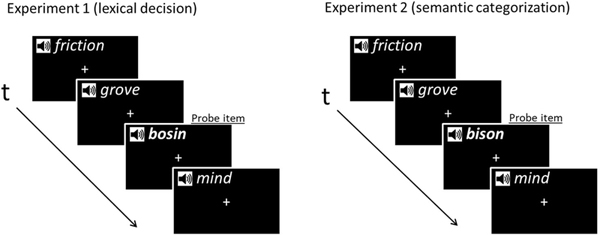
Procedure for both of the experimental tasks with an example of a prime item for each. Items were identical between the two tasks except for the probe items which were either animal names for semantic categorisation, or non-words for lexical decision made from transposed versions of animal names.

For this experiment, each participant completed two blocks of a go/no-go lexical decision task that alternated with two blocks of a go/no-go semantic categorisation task (see Experiment 2 - note the probe items were changed for Experiment 2). The order of blocks was counterbalanced across participants and every critical word was presented in each task across participants. In the current experiment, participants were instructed to press a button on a game controller as soon as they heard a stimulus that was not a legal English word (pseudoword probes). The non-words probes made up approximately 13% of trials. The critical words made up the other 87% of trials and did not require a behavioural response.

EEG recording

The electroencephalogram (EEG) was collected using a 29-channel electrode cap containing tin electrodes (Electro-Cap International, Inc., Eaton, OH), arranged in the International 10–20 system (see Figure 2). Electrodes were also placed next to the right eye to monitor horizontal eye movements and below the left eye to monitor vertical eye movements and blinks. And finally, two electrodes were placed behind the ears over the mastoid bones. The left mastoid site was used as an online reference for the other electrodes and the right mastoid site was used to evaluate differential mastoid activity. Impedance was kept below 2.5 kΩ for all scalp and mastoid electrode sites and below 5 kΩ for the two eye channels. The EEG signal was amplified by SynAmpsRT amplifier (Neuroscan-Compumedics, Charlotte, NC) with a bandpass of DC to 200 Hz and was continuously sampled at 500 Hz.

Figure 2.

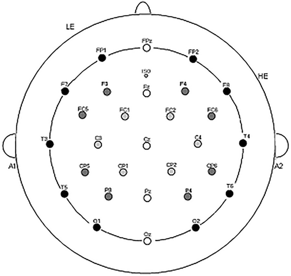
Electrode montage used for EEG recordings.

Data analysis

While a traditional factorial approach to analyzing these data would have substantial power due to the high number of subjects and items, as mentioned previously this approach is highly susceptible to confounds due to uneven distribution of values between variables. The typical approach to dealing with such confounds is to arrange the stimuli in a factorial design such that the effects of each variable are controlled across the levels of the other variables. The problem here is that with four factors each with several levels, even with almost a thousand items there would be comparatively few items per cell in the design and this still assumes that enough items can be found to meet the rigid criteria of each such cell. To help overcome this problem the data were analyzed by constructing linear mixed effects regression models using the Ime4 package (Bates, Maechler, Bolker, & Walker, 2015) written in the statistical computing language R (R core team, 2014). Rather than averaged ERP data, for these analyses we used the single trial EEG data (after artifact rejection) from 50 participants, 956 items, and 29 electrode sites as input to the analyses. The structure of the models used was based on the approach recommended by Payne et al. (2015).

A set of eight identical LME models were fit for eight consecutive 100 ms time windows starting at 100 through to 900 ms post word onset. The main effects included in the models were the word variables; Lexical Frequency, PLD, Concreteness and Duration. The word variable measures were normalised (z-scores) prior to fitting the LME models (Payne et al., 2015). Distributional effects were modelled using the relative position of each electrode in three dimensional space using three continuous variables, corresponding to the X, Y, and Z coordinate position of each of the 29 scalp sites. For the X-position variable, the left and rightmost electrode sites (T3 and T4) had the most extreme values and interactions with this variable would indicate differences in the laterality of an effect. Conversely for the Y-position variable, the most anterior and posterior electrodes (FPz and Oz) represent the most extreme values and interactions here indicate a difference in how anterior/posterior an effect is distributed. The-Z position variable varies from a maximum at the central electrode Cz at the top of the head and descends to the outer ring of peripheral sites (from FPz to T3 to Oz to T4 and back to FPz), marking the two extremes. Interactions involving the Z-position factor indicate differences in the elevation of an effect. The two-way interactions were structured so each word variable had three possible two-way interactions, one with each of the three distributional variables (X, Y, and Z position). The overall effects of these distributional variables were also added into the models as covariates.

It should be noted that distributions of actual ERP effects are non-linear, and this limits the ability of linear models to appropriately analyze scalp distribution. ANOVA approaches generally model distribution by assigning electrode sites to separate levels of discrete distributional variables (e.g “laterality”). This allows for non-linearity, but introduces a number of issues that come with discretizing a continuous variable and using ANOVAs to analyze effect distributions (e.g. MacCallum, Zhang, Preacher, & Rucker, 2002; McCarthy & Wood, 1985). The current approach allows us to approximate the distribution of an effect as the extent to which it fits one of the 3 spatial dimensions. This encompasses some general ERP distributions (e.g. the typically centralised N400 distributions) but results in a greater degree of model misfit (and thus inflated type-2 error rate) for effects which have smaller or more complex distributions (see Tremblay & Newman, 2015). Nonetheless, any further specification of distributional factors would not be justifiable without stronger predictions.

Because of the complexity of the design, a maximal random effect structure was not possible due to convergence failures (Barr, Levy, Scheepers, & Tily, 2013). Instead, based on a model selection approach recommended by Matuschek, Kliegl, Vasishth, Baayen, and Bates (2017), random effects were structured to be conservative, yet still allow every model to converge. The resulting random effect structure for each model included random intercepts for participants, items, and electrode channel as well as by-subject random slopes for the effect of each of the four experimental variables (see appendix for model code).

The 95% profile likelihood confidence intervals and t-values were calculated for each comparison (Cumming, 2014). Because of the large number of comparisons, p-values from each model were also obtained using the “Anova” function in the CAR package (CRAN) which were then false-detection-rate (FDR) corrected using the MATLAB “Mass Univariate ERP Toolbox” (Groppe, Urbach, & Kutas, 2011). To add another level of conservation, effects were only interpreted as significant if the comparison was significant for both the confidence intervals and the FDR-corrected ANOVA p-values.

Data visualization

We also used LME models to compute the equivalent of scalp voltage maps to help in visualising the various effects in each model. For these analyses we used the same approach as above but instead of including distributional variables in each model, we computed separate LME solutions for each of the 29 scalp sites in each 100 ms time epoch and plotted the resulting LME t-statistics across the scalp using interpolated topographic maps (see appendix for individual site model code).

Additionally, ERPs were used to aid in the interpretation of results. Similar to a traditional factorial approach, averaged ERPs time-locked to stimulus onset were created off-line as a function of each of the variables of interest (Frequency, PND, Concreteness and Duration). For each of these variables the data were sorted into four equally spaced levels which resulted in 239 trials per level. Trials with muscular or ocular artifact were rejected prior to averaging. The left mastoid was used as the reference electrode and averaged data were baselined using the mean voltage between −100 and 0 ms at each site. The averaged ERPs plotted in Figures 3–6 show the highest and lowest quartiles for each variable of interest per experiment. Note that these comparisons are only for visual reference and do not control for the influence of the other variables or random effects.

Figure 3.

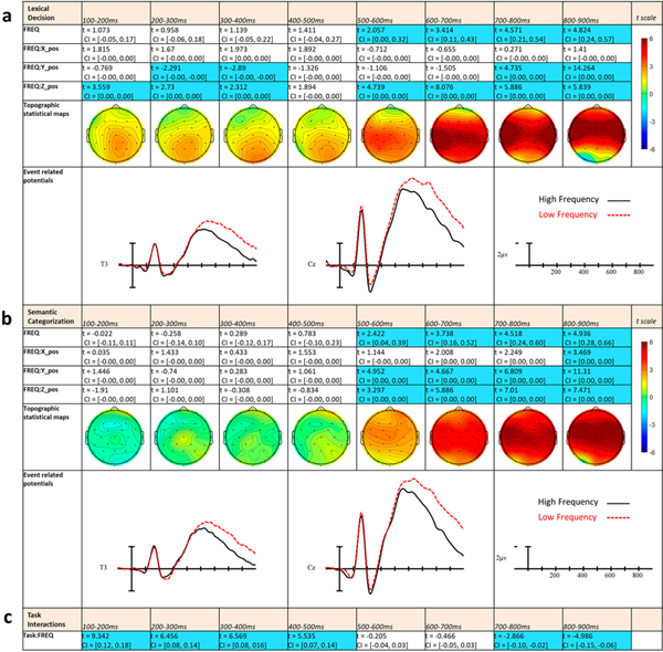
LME t statistics, confidence intervals, topographical LME t-statistic maps, and ERPs representing the Frequency effects for Experiment 1 (a) and Experiment 2 (b). Effects are only highlighted if significant with both confidence intervals and FDR-corrected p-values. ERP plots were made using the top and bottom quartiles of items sorted by frequency. (c) Statistics from task comparisons using separate LME models including task.

Figure 6.

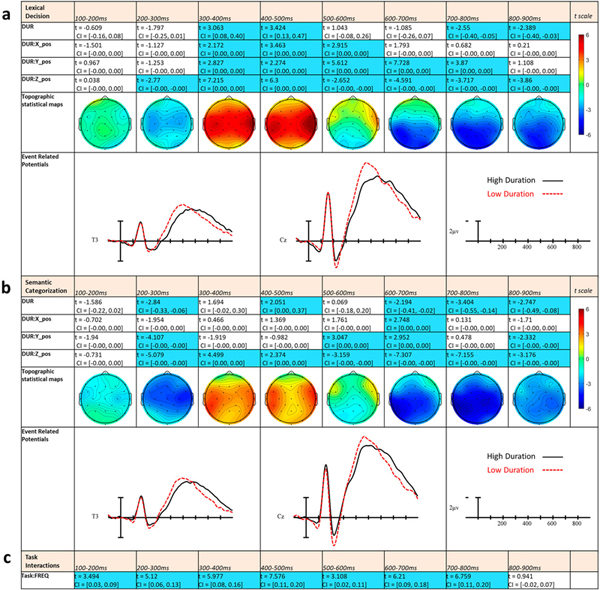
LME t statistics, confidence intervals, topographical LME t-statistic maps, and ERPs representing the Duration effects for Experiment 1 (a) and Experiment 2 (b). Effects are only highlighted if significant with both confidence intervals and FDR-corrected p-values. ERP plots were made using the top and bottom quartiles of items sorted by Duration. (c) Statistics from task comparisons using separate LME models including task.

Results

Linear mixed effect model results

Due to the number of results, the confidence intervals and t statistics for each comparison are presented in a series of tables for each variable (Frequency, PND, Concreteness, and Duration). Effects are highlighted only if the comparison was significant for both the confidence intervals and the FDR-corrected ANOVA p-values. Included in each table are statistical topographic maps created by single-site LME effect estimates calculated per electrode and task, using the same models as described above with the removal of the distributional variables. Also included for visual comparison are averaged ERPs comparing the highest and lowest quartile of each variable for a central (Cz) and a lateral (T3) electrode site.

Frequency effects

Starting in the first epoch from 100 to 200 ms there was a Frequency by Z-position interaction. This pattern indicates that along the continuum of word frequencies, items towards the lower end of the scale tended to produce greater ERP negativity than items towards the higher end and that this effect was larger towards the top of the head (see Figure 3a). In the following 200–300 ms epoch, the previous interaction remained and there was also a Frequency by Y-position interaction, suggesting the frequency effect was now more concentrated over posterior electrode sites. In 300–400 ms epoch these two two-way interactions remained however in the following 400–500 ms epoch there were no effects of Frequency. In the 500–600 ms epoch the frequency effect re-emerged and was significant as both a main effect as well as a Frequency by Z-position interaction. This indicated a strong, widespread frequency effect that was largest at central electrode sites. In the last three epochs (600–900 ms), these two effects remained significant, but in the 700–800 ms and 800–900 ms epoch there were also Frequency by Y-position interactions indicating the distribution shifted towards the front of the head in later epochs.

Phonological neighbourhood density effects

In the initial 100–200 ms epoch there were no effects of PND. Starting in the 200–300 ms epoch there was a main effect of PND such that words with larger phonological neighbourhoods tended to produce greater negativity than words with smaller phonological neighbourhoods. This neighbourhood effect interacted with all three distributional variables and appears to reflect a wide distribution across the central line of electrodes which was larger on the right of the montage (see Figure 4a). In the following 300–400 ms epoch there was a PND × Z-position interaction, reflecting a small reversal of the effect in central sites, with more negativity now for words from low density neighbourhoods (see map in Figure 4a). In the 400–500 ms epoch, there were no effects of PND or any interactions. Then, beginning in the 500–600 ms epoch and continuing through the rest of the epochs, there were PND by Z-position interactions showing greater negativity to words with dense phonological neighbourhoods, especially in central sites. Additionally, in only the 500–600 ms time window there was a PND by Y-position interaction, reflecting a more anterior distribution of the effect and perhaps indicating that this epoch is where the later PND effect is the strongest.

Figure 4.

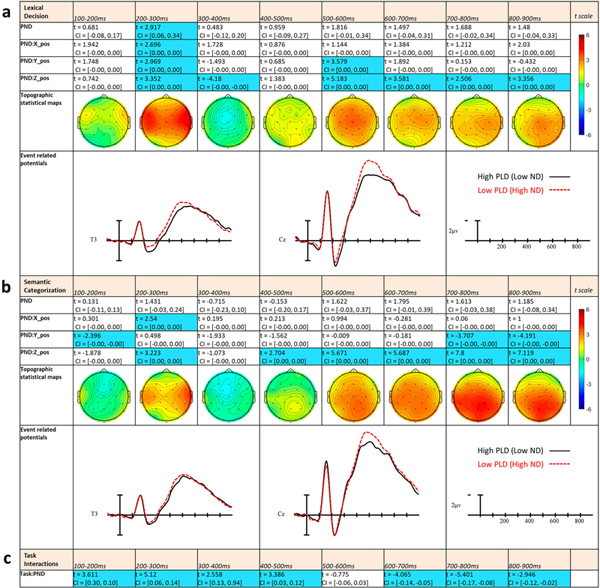
LME t statistics, confidence intervals, topographical LME t-statistic maps, and ERPs representing the PLD (PND) effects for Experiment 1 (a) and Experiment 2 (b). Effects are only highlighted if significant with both confidence intervals and FDR-corrected p-values. ERP plots were made using the top and bottom quartiles of items sorted by PND. (c) Statistics from task comparisons using separate LME models including task.

Concreteness effects

In the initial three epochs there were no effects of Concreteness. In the 400–500 ms epoch there was a Concreteness by X-position and a Concreteness by Z-position interaction, demonstrating greater negativities to higher concreteness words with the effect more concentrated on the central-left side of the montage (see Figure 5a). These effects continue into the 500–600 ms epoch, with the addition of a main effect of Concreteness. In the following 600–700 ms epoch, the interaction between Concreteness and X-position switches to a Concreteness by Y-position indicating the effect now has a more posterior distribution. In the last two epochs from 700 to 900 ms, the effect remains as Concreteness by Z-position interactions and is still centrally distributed around the top of the head.

Figure 5.

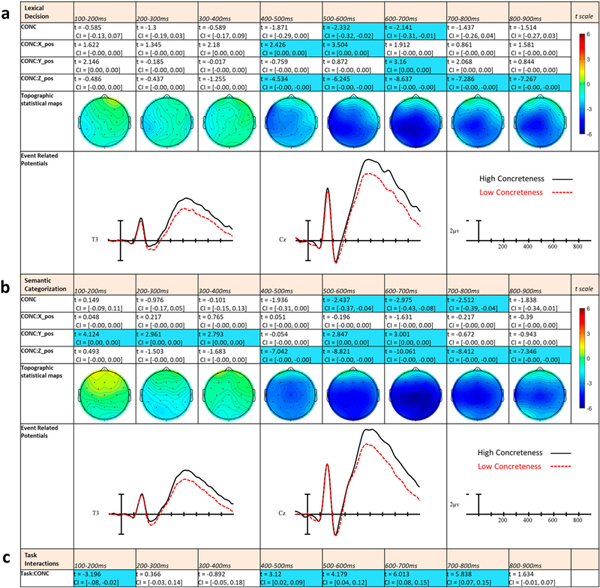
LME t statistics, confidence intervals, topographical LME t-statistic maps, and ERPs representing the Concreteness effects for Experiment 1 (a) and Experiment 2 (b). Effects are only highlighted if significant with both confidence intervals and FDR-corrected p-values. ERP plots were made using the top and bottom quartiles of items sorted by Concreteness. (c) Statistics from task comparisons using separate LME models including task.

Duration effects

The effects of word duration started in the 200–300 ms epoch where Duration interacted with Z-position. Here the effect showed greater negativity for longer than shorter duration words (see Figure 6a). During the next two epochs, 300–400 ms and 400–500 ms, there were main effects of Duration as well as distributional interactions showing the direction of the effect has reversed, with shorter words now producing more negativity. This effect was distributed perpendicular to the midline, especially in the rightmost sites. In the following 500–600 ms epoch, there was no main effect for Duration, however distributional interactions suggested that lateral right sites still showed remnants of the previous effect while in posterior sites the effect reversed once more, such that longer words elicit more negativity. In the remaining three epochs, this posterior effect grew in size and magnitude and became significant as a main effect in the 700–800 ms epoch with longer words producing greater negativities than shorter words. This pattern is especially apparent in the ERP plots in Figure 6a, and appears to be due to a shift in the latency of the N400 - shorter duration words producing a shorter N400 time-course.

Behavioural results

During Experiment 1, participants correctly detected, on average, 77% of non-word probes with false alarms on 3% of critical trials. Reaction times for correct lexical decision judgments averaged 967 ms (SD = 188 ms).

Discussion

In Experiment 1, we found independent effects of four different word-based variables on the continuous processing of spoken words during a go/no-go lexical decision task. This included temporally and spatially widespread effects of word frequency, phonological neighbourhood density, concreteness and word duration. For word frequency, there was an increase in ERP negativity associated with decreases in word frequency. These effects began in the 100–200 ms epoch and became more exaggerated after 500 ms, near the peak of the auditory N400 (see Figure 3a). A somewhat different picture emerged for the phonological neighbourhood density (PND) variable. Here we found an early effect between 200 and 300 ms with greater negativity associated with increases in phonological neighbourhood density, and then a small reversal (dense neighbourhoods eliciting more positivity) in the 300–400 ms epoch. However, in the timeframe of the N400 (500–900 ms), the pattern reverted to greater negativity for denser phonological neighbourhood words (see Figure 4a). For concreteness, we found a widely distributed pattern of larger negativities associated with words rated as more concrete, and this pattern started in the 400–500 ms epoch and persisted through 900 ms (see Figure 5a). Finally, there were also widespread effects of the duration of the spoken words. As can be seen in Figure 6a, this pattern appears to result mostly from a shift in the temporal distribution of the N400, with words of shorter duration resulting in an N400 that starts and ends earlier than the comparable effect for longer words. The one departure from this pattern is the centrally distributed larger negativity for long words in the 200 to 300 ms epoch. This effect could be due to a larger P2 component for the shorter words.

Experiment 2 (semantic categorization)

Experiment 2 contains data from the same words and participants as Experiment 1, but instead of the lexical decision task, here we used a go/no-go semantic categorisation task (SC) which required subjects to determine if words were members of a specific semantic category (animals). Prior research has shown that experimental task can impact word processing in a variety of contexts. For instance, semantic priming has more of an effect on the auditory N400 during a memorisation task compared to a counting task, indicating that the N400 is not impervious to top-down influences (Bentin, Kutas, & Hillyard, 1993). Relevant to the current variables of interest, recent studies with written words have shown that the ERP effects of word frequency (Strijkers, Bertrand, & Grainger, 2015) and concreteness (Chen et al., 2015) are modulated by experimental task. Compared to lexical decision, a task like semantic categorisation that focuses participants’ attention to the semantic attributes of each word may have a larger impact on later meaning-sensitive ERP components such as the N400.

Method

The methods for the second experiment were identical to those of Experiment 1. The data were collected from the same subjects, in the same recording session as Experiment 1. The same set of 960 critical words and data collection procedures were also used. The only procedural difference was that the task during the two blocks of trials in this experiment was changed from lexical decision to semantic categorisation. This necessitated changing the 140 pseudoword items from Experiment 1 to 140 animal names in Experiment 2. These items were digitally recorded and edited using the same parameters as the critical word stimuli. Participants were told to press a designated button whenever they heard an animal name and to withhold responding to all other (critical) words (go/no-go semantic categorisation).

The resulting data were analyzed from the same eight time windows as in Experiment 1 and the structures of the LME models were identical to those constructed for the lexical decision task, with the only difference being that they were fit using the semantic categorisation data.

Results

As with Experiment 1, the confidence intervals and t statistics for each comparison are presented in a series of tables for each variable (Frequency, PLD, Concreteness, and Duration) below the results for Experiment 1. Effects are highlighted only if the comparison is significant for both the confidence intervals and the FDR-corrected ANOVA p-values. Included in each table are topographic statistical maps created by single-site LME model t statistics and averaged ERPs comparing the highest and lowest quartile of each variable for a central (Cz) and a lateral (T3) electrode site.

Frequency effects

In Experiment 2, there were no effects of Frequency in the first four epochs. Beginning in the 500–600 ms epoch, there was a main effect of Frequency as well as a Frequency by Z-position and a Frequency by Y-position interaction which showed that greater ERP negativities were associated with lower frequency words primarily in central and frontal electrode sites (see Figure 3b). These effects persisted through the final epoch, with the addition of a Frequency by X-position interaction in the 800–900 ms epoch, indicating an increasingly strong and widespread frequency effect.

Phonological neighborhood density effects

In the first epoch there was an interaction between PND and Y-position, probably due to a small negativity to low density words at frontal sites (see Figure 4b). Following in the 200–300 ms epoch there was a PND by X-position interaction and a PND by Z-position interaction, resulting from greater negativities associated with increases in neighbourhood density, especially over the central line and right hemisphere electrodes. The following epoch (300–400 ms) there were no significant effects of PND. In the 400–500 ms epoch there was again a PND by Z-position interactions in the same direction as the previous effect, though now distributed more centrally. This effect remained significant through the rest of the epochs, with the addition of a PND by Y-position interaction in the 700–800 ms and 800–900 ms epochs as the effect became more focused in posterior sites.

Concreteness effects

There were small Concreteness by Y-position interactions through the first three epochs (100–400 ms), with more concrete words producing greater ERP negativities in posterior sites. Starting in the 400–500 ms epoch, larger and more wide-spread concreteness effects emerged as Concreteness by Z-position interactions. This pattern lasted for the rest of the measured epochs and reflected a distribution focused on the top of the head. From 500 to 800 ms there were also main effects of Concreteness indicating these were the epochs with the strongest and most widespread concreteness effects (see Figure 5b). Additionally, in the 500–600 ms and 600–700 ms epochs there was a Concreteness by Y-position interaction indicating the effect was stronger in posterior sites.

Duration effects

The effects of Duration started in the 200–300 ms epoch, where there was a main effect and distributional interactions reflecting greater negativity to higher duration words in all but the most posterior sites (see Figure 6b). Between 300 and 500 ms there were Duration by Z-position interactions, although importantly in these epochs, the direction of the effect switched polarity; shorter duration words produced more negativity. In the following 500–600 ms epoch there was a Duration by Z-position and a Duration by Y-position interaction showing the pattern of Duration effects again flipped such that longer words produced more negative ERPs, especially in posterior-central sites. The Duration effect remained significant through 900 ms as distributional interactions and in the final two epochs, as main effects, indicating a widespread, central-posterior distribution of the later Duration effect.

Behavioural results

During Experiment 2, participants correctly detected, on average, 84% of animal probes with false alarms on approximately 1% of critical trials. Reaction times for correct semantic categorisation judgments averaged 847 ms (SD = 186 ms).

Discussion

Experiment 2 used the same critical items, procedure, and model structure as Experiment 1 except for the experimental task, which was semantic categorisation rather than lexical decision. Overall, the results were similar to Experiment 1, with frequency, PND, concreteness, and length all producing effects, although there were a few notable differences. In Experiment 2, there were no early frequency effects. Frequency only became significant after 500 ms, where high frequency words elicited less negativity than low frequency words (see Figure 3b). For PND, effects were observed early, in the first two epochs, and again later, after 400 ms, with words with larger neighbourhoods generating greater negativities than words with smaller neighbourhoods (see Figure 4b). There were small early effects of concreteness, but larger and more robust effects after about 400 ms, where concrete words elicited larger negativities than abstract words (see Figure 5b). Effects of duration were found across all epochs after 200 ms similar to Experiment 1. Shorter words produced more positivity in the 200–300 ms epoch, reflecting larger P2s. In the next two epochs shorter words produced more negativity than longer words, followed by the reversed pattern in the final four epochs, reflecting an earlier onset of the N400 for shorter words compared to longer words (see Figure 6b).

Task comparisons

To compare the results from each task, a set of simplified task models were constructed and fit using the data from both Experiment 1 and 2. These models were structured such that they contained the same random effects and main fixed effects as the previous individual task models of Experiment 1 and 2. However, we also added two-way interactions between task and each experimental variable. To keep the structure of the models manageable we did not include interactions with distributional variables (see appendix for task model code). Thus, these task models analyze differences in the experimental variable main effects between the two tasks across all electrode sites, but they do not analyze how the distributions of these effects might differ across tasks. The results of these models are included in the figure for each variable, below the two tasks (Figures 3–6).

Task interacted with Frequency in the first four epochs (100–500 ms), suggesting that there was a greater effect of Frequency during LD than SC. Indeed, inspection of the maps in Figure 3 shows a significant early effect of Frequency in Experiment 1, but no such effect in Experiment 2. There were no interactions between Task and Frequency in the following two epochs (500–700 ms), although in the final two epochs (700–900 ms), there was again an interaction between Task and Frequency. However, the interactions in the last two epochs suggest that the Frequency effect was stronger or more widespread during SC than LD (note the flipped t statistic).

In the 100–200 ms, 200–300 ms and 400–500 ms epochs there were interactions between Task and PND showing a larger overall effect of PND in these epochs during the LD task compared to SC task (see Figure 4). There was not a Task by PND interaction in the 300–400 or 500–600 ms epochs. In the final three epochs (600–900 ms) there were also Task by PND interactions, however now these interactions indicated it was the SC task which produced the larger PND effect.

Task and Concreteness interacted in the initial epoch (100–200 ms) due to a greater overall positive effect in SC combined with an overall negative effect in LD (see Figure 5; the concreteness main effect t-values). For the following 2 epochs (200–400 ms) there were no interactions between Task and Concreteness. Then for the next four epochs (400–800 ms) there was a Task by Concreteness interaction indicating a larger effect of Concreteness during SC compared to LD.

For Duration, there were widespread interactions with Task starting in the 100–200 ms epoch and extending to the 700–800 ms epoch. These interactions followed a pattern in which there were greater effects of Duration during SC when the effect was in the negative direction (lower duration words producing less negativity). When the effect was in the positive direction (lower duration words producing more negativity), the effect was larger for LD than SC.

General discussion

In this study 50 participants were presented with approximately a thousand spoken words in two experiments that differed only in the task participants engaged in. In Experiment 1 participants made go/no-go lexical decisions to each item, pressing a button to occasional (13% of items) non-word probes. In Experiment 2 participants made go/no-go semantic categorizations to each item, pressing a button to occasional (13% of items) animal name probes. The remaining 960 trials in both experiments contained the same critical word items that did not require a behavioural response and therefore the ERPs to these reflect auditory word processing unbiased by overt motor responses. We measured ERPs in eight consecutive temporal epochs starting at 100 ms and ending 900 ms after word onset for each of the 956 critical words in the two experiments. LMER analyses were used to examine the independent effects of four variables (word frequency, phonological neighbourhood density, concreteness, and word duration) on the time-course of ERP measures of spoken word processing. Consistent with a variety of previous studies, including one that used the same basic approach and materials with written words (Dufau et al., 2015), we found that all four variables produced robust effects on mean EEG amplitude measures across the range of latencies examined. While the two experiments produced a similar overall pattern of effects there were also subtle differences in the precise time course of effects in the two experiments.

Word frequency

In both the lexical decision (Experiment 1) and semantic categorisation (Experiment 2) tasks there were robust effects of word frequency across a range ERP latency windows. In both experiments the relationship between word frequency and ERP mean amplitude was the same with less frequent words tending to produce greater ERP negativities than more frequent words (see Figure 3). Remarkably, Experiment 1 found effects of frequency as early as the first measured epoch, 100–200 ms, with lower frequency items generating larger negativity around the vertex of the scalp. To our knowledge this early effect has not been observed during other studies of auditory word recognition, although a similar pattern has been reported for visual word recognition (e.g. Chen et al., 2015; Hauk et al., 2006). Dufour et al.’s auditory study did find an effect in a 330–400 ms epoch although of opposite polarity to typical ERP frequency effects. The current study used a much larger sample of words with greater variance than Dufour et al., perhaps explaining why effects were found much earlier.

Though perhaps useful for the interpretation of later frequency effects, the early onset of the frequency effect is clearly incompatible with certain early explanations of word frequency effects such as it represents only a response bias (Balota & Chumbley, 1984) or a post-lexical selection bias (Luce & Pisoni, 1998). These earliest effects of frequency indicate that word frequency impacts initial phonological processing, even before the entire word has been heard. In connectionist models such as TRACE (McClelland & Elman, 1986), this effect could be explained by the greater activation level of higher frequency lexical representations sending more feedback to sub-lexical phonological representations, and thus reinforcing the activation of these units (see also, Gaskell & Marslen-Wilson, 1997). In these models, as well as Bayesian models (e.g. Norris & McQueen, 2008), the early effect of frequency could reflect higher phonetic probability of the initial phonemes of high frequency words, affecting the amount of necessary activation at the level of sublexical nodes or connections. In any case, these frequency effects add to the body of research suggesting that word frequency effects can occur prior to N400 onset (e.g. Assadollahi & Pulvermüller, 2003; Hauk et al., 2006; Hauk & Pulvermüller, 2004; Sereno et al., 1998) and extends them to the spoken word processing domain.

Interestingly, these early frequency effects were only present during the lexical decision task (Experiment 1) and not semantic categorisation (Experiment 2). A similar dissociation was recently obtained for written words by Strijkers et al. (2015) who reported effects of word frequency that emerged earlier during a semantic task (150 ms) than during a colour discrimination task. They attributed this discrepancy to differences in the depth of processing, but this explanation may not be sufficient for the current findings, since the words in both LD and SC still need to be fully recognised. Here, the interaction may reflect the influence of task demands on early sublexical or lexical processing. Lexical decision may focus participants’ attention to the sublexical/lexical properties of the items in order to quickly perform the task, while during semantic categorisation, attention might be focused more on the conceptual properties of words which presumably become available later in the time course of spoken word processing. Broadly speaking, this task difference in word frequency provides strong evidence supporting the idea that even early stages of word recognition are affected by top-town influences.

The most prominent effect of word frequency was found on the auditory N400 component where higher frequency words elicited less negativity than lower frequency words in both Experiment 1 and 2. This has been widely found in the visual domain (e.g. Dufau et al., 2015; Van Petten & Kutas, 1990), though in the auditory domain, ERP studies of word frequency are limited. As mentioned above, one study (Dufour et al., 2013) has looked at word frequency effects on spoken word ERPs. While they did not find early effects of frequency like the current study, they did report an N400 effect between 550 and 650 ms epoch for auditory words. This is about the time frame in which the word frequency effect in the current study dramatically increases in size (see Figure 3). One possible interpretation of the pattern seen here is that the N400 frequency effect represents similar processes in both written and spoken word recognition, but tends to have a stronger later impact on spoken word processing due to the temporal dynamics of spoken word recognition. For example, if the N400 reflects the process of mapping lexical onto semantic representations as proposed by Grainger and Holcomb (2009), because this process likely extends over much of the temporal extent of a spoken word, this process is likely to have a longer timeframe to exert its influence. Another possibility is that the extended spoken word N400 effects could reflect in part the greater temporal variability of individual N400s to the different items used (see, Holcomb & Neville, 1990 for a similar explanation).

Some accounts of N400 frequency effects suggest that they reflect changes in the activity of lexical representations as a function of word frequency, with greater activity for more frequent words (for instance in models like Trace or Cohort and their descendants). Other explanations focus on the semantic nature of the N400, suggesting greater N400s to low frequency words represents the greater activation necessary to access their semantic networks (Kutas & Federmeier, 2011), potentially due to having fewer or weaker connections within their semantic network. In the current study, the later half of the N400 frequency effect (after 700 ms) was larger, or at least more widespread, during semantic categorisation. Since semantic categorisation likely necessitates additional semantic processing, this pattern seems to favour a semantic explanation of the later frequency effect, or at least provides evidence that part of the N400 frequency effect is due to differences in processing within semantic systems.

Phonological neighborhood density

Across experiments, effects of PND were found in an early 200–300 ms epoch as well as in later epochs starting at 500–600 ms. The nature of these effects was that words with many lexical neighbours tended to produce more negative-going ERPs than words with fewer lexical neighbours. The earlier effect was largely isolated to one epoch, roughly corresponding to the auditory P2, and was focused on right lateral sites extending across the central line of electrodes to left lateral sites (see Figure 4). Neighbourhood effects in similar time frames have been observed in several studies using visually presented words (e.g. Midgley, Holcomb, Walter, & Grainger, 2008; Vergara-Martínez & Swaab, 2012). However, the two ERP studies investigating PND effects conducted in the auditory domain have not shown the effect seen in the current study. Both Dufour et al. (2013) and Hunter (2013) found early PND effects surrounding the P2 component, however in both cases the patterns they reported were in the opposite direction (larger positivities to larger phonological neighbourhoods) to those found here. The discrepancy between these two studies and the present study could be accounted for by differing methods. Besides concerns inherent with factorial designs (e.g. smaller number of items per condition, covariance between variables) and methodological choices (e.g. the use of an average reference in Dufour et al., 2013), there were differences in how PND was measured. Both of these prior studies used short words with the traditional measure of neighbourhood density (Vitevitch & Luce, 1998) and PND conditions in these studies co-varied with phonotactic probability. These variables are correlated since the phonemes in words with many neighbours are more likely to be heard, but interestingly the effects these two variables have on word recognition and ERPs may be opposite. While higher PND generally is thought to interfere with word recognition due to increased competition between words, phonotactic probability may facilitate processing via a more frequent sublexical phonology in terms of phoneme frequencies or transitional probabilities between phonemes. Thus the early effect in the two prior studies may reflect an effect of phonotactic probability, and thus share an explanation similar to early frequency effects such as increased connection strength between more frequent sublexical units. Phonotactic probability and PND are still correlated in the present study, but less so than in the other two since we included a wide range of word lengths and used PLD20 as the measure of neighbourhood density which encompasses larger-scale neighbourhoods than the traditional neighbourhood density measure (Yarkoni et al., 2008). Additionally, there was a much greater range of PND values in the current study, and effects of other variables like word frequency were controlled for. Hence the early effect in the current study could reflect co-activation of phonological neighbour’s sublexical or lexical networks, perhaps driven by words with many cohorts.

This early effect (200–300 ms) was larger in Experiment 1 (LD) than Experiment 2 (SC). Similar to the interactions between frequency and task in this timeframe, this could indicate the ability of task demands to emphasise certain levels of processing. If this early effect represents sublexical or lexical co-activation, it could be amplified by attentional processes scrutinising every phoneme of the incoming input in order to better complete the more difficult lexical decision task. Meanwhile, participants doing semantic categorisation might withhold scrutiny until later processing stages. Further, during lexical decision, input needs to be compared with many more potential targets (every real word) than for semantic categorisation, which only needs to be compared with one semantic category. Thus a lexical-level effect might have a smaller early component during semantic categorisation because the task constrains the number of words which need to be compared with to successfully participate in the task. Regardless, this pattern again indicates that task demands affect relatively early phonological processing, perhaps due to some pattern of constraining feedback activity during semantic categorisation, or increased overall attention during lexical decision.

The later effect beginning at 500 ms likely reflects an influence of PND on the auditory N400. This has been found during visual word recognition, where words from large orthographic neighbourhoods generate larger N400s than words from smaller neighbourhoods (e.g. Holcomb et al., 2002; Laszlo & Federmeier, 2011). In the auditory domain, one prior study has found this effect of PND in a 550–650 ms epoch (Dufour et al., 2013), however another study found no effect of PND on the N400 (Hunter, 2013). For the later N400 effect, it seems likely that neighbourhood effects for both visual and auditory words would share similar explanations. That is, high density words cause greater co-activation of phonological or orthographic neighbours than low density words. With more activation in lexical-semantic networks, the target word requires more activation to be recognised and has more neighbours to inhibit. This increases the time and effort for the word recognition system to arrive at the correct word, leading to increased negativity on the N400 (Holcomb et al., 2002). Given its dynamic nature, neighbours may exert more long lasting influence during spoken word recognition compared to written word recognition. Especially for words with many cohorts, high density spoken words likely partially activate neighbours all the way to their semantic representations, before the entire word has been heard.

In the current study, this later effect of PND lasts until 900 ms, and was larger for SC (Experiment 2) than for LD (Experiment 1), providing more evidence that phonological neighbours in spoken word recognition co-activate to the point of their semantic representations. This also supports the interpretation that the earlier Task by PND interaction (200–300 ms) was in due to participants (covertly or overtly) focusing greater concentration during LD in early processing stages and in later stages for SC. Overall the finding of two separate PND effects, each of which interact oppositely with Task, suggests that for spoken word recognition neighbourhood density impacts processing in at least two stages, a pre-recognition “first-pass” perhaps driven by greater numbers of cohorts or other predicted words, and a later, longer lasting, lexical-semantic stage possibly driven by the inhibition of lexical competitors and the co-activation of semantic information.

Concreteness

Across both experiments there were robust effects of concreteness between 400 and 900 ms after word onset and this effect was widely distributed around central sites. Although there are no published studies of ERPs to spoken words as a function of concreteness the pattern seen here is similar to the ERP effects reported in the written word recognition literature. For visual words, N400 effects have been shown across a variety of tasks and language contexts (e.g. Kounios & Holcomb, 1994; Holcomb et al., 1999) with larger N400s for words rated as being more concrete and smaller N400s for more abstract words. This pattern is usually interpreted as reflecting the richer semantic neighbourhoods, including those reflecting imagistic representations, engaged by words representing concrete concepts (Holcomb et al., 1999). That spoken words access a similar set of semantic representations as written words is consistent with a common semantic system architecture that is assumed by most models of word recognition (e.g. the BIAM of Grainger & Holcomb, 2009). Interestingly this effect of concreteness interacted with task such that it was stronger during SC than LD in the epochs between 400 and 800 ms. This follows a similar pattern as the later effects of frequency and PND which were also larger for SC than LD. Thus, it might share a similar explanation having to do with additional, or deeper, processing at later semantic levels during SC which affords more opportunity for concreteness effects.

One peculiarity of the concreteness effects was that in Experiment 2 there were significant distributional interactions with Concreteness as early as the 100–200 ms epoch. Examination of the statistical maps on Figure 5, suggests these interactions may be due to a graded effect of concreteness across the midline, originating in occipital sites where more concrete words produced more negativity. The same comparisons in Experiment 1 were not significant. Given the timeframe, these earlier and weaker concreteness effects seem at first blush to be unlikely to be the result of an actual semantic concreteness effect (like the N400 effect), but rather may have to do with some physical property of more concrete or abstract words which was not in the LME models. That said, the presence and distribution of this early effect seems to be influenced by experimental task, suggesting that whatever the explanation is, it is not independent of top-down influences. Consistent with the top-down task explanation is the possibility that the SC task focused participants on the semantic level of analysis and therefore, like the early frequency and PND effects for LD, might have resulted in an early difference due to concreteness. This could in theory happen in a design with a lot of power if even a relatively small subset of items had an early cue to their semantic attributes.

Duration

In both Experiment 1 and 2, effects of duration were found across all epochs after 200 ms and are best understood by examining the duration ERP plots in Figure 6. The initial effect (200–300 ms) appears to be due to larger P2s to shorter words compared to longer words. This is the opposite of what has been found with visual word recognition which finds increased activity to longer words than shorter words in early components (e.g. Dufau et al., 2015; Hauk & Pulvermüller, 2004). This discrepancy between the two modalities makes sense given that it is likely that the amplitude of early ERP components is concordant with the amount of information present. Visually, longer words present more information at once and consequently may explain larger early components. However, for spoken words the information from longer items is not simultaneously present. Here, it is possible that the positivity to shorter words is due to a relatively larger, or more quickly revealed, amount of information compared to longer words especially during earlier epochs.

In the 300–400 and 400–500 ms epochs, the direction of the effect switched such that shorter words produced larger negativities than longer words. This is likely due to the faster onset of N400 activity to shorter words due to their faster temporal properties. Meanwhile for longer words, the word recognition system is still waiting on additional information to fully process these items leading to later and more spread-out N400 processing. Consistent with this interpretation, in the 500–600 ms epoch there is another switch in the direction of the duration effect. In these later epochs, there are greater negativities for longer compared to shorter words because the N400s of shorter words offset faster than the N400s of longer words.

Interestingly, there were widespread interactions between Task and Duration through 800 ms. Overall this is due to a larger duration effect during LD between 100 and 300 and between 500 and 800 ms, separated by a larger effect during SC between 300 and 500 ms. This pattern seems to be related to differences in the ERPs of longer duration words which are more negative during SC, while the ERPs for shorter words appear similar (see ERPs in Figure 6). Though difficult to interpret, one possibility is that if during lexical decision recognition systems are attempting to work faster to deal with the more involved task, this may further increase the difference in component timing between shorter and longer words for LD compared to SC. Shorter words in the LD task transition faster from early processing phases to N400 processing, leading to a smaller duration effect on the P2, and a larger effect in early N400 epochs because the direction of these effects have opposite polarity.

Conclusions

Methodologically, this study further demonstrates the effectiveness of large-scale item based analysis strategies for the understanding of word recognition processes. The LMER models revealed intricacies in the time course of the effects which would be normally obscured by the averaging processes of factorial designs. Further, for multi-dimensional stimuli such as words, the ability to control for collinearity between variables as well as subject, item, and electrode level random effects is critical for the understanding of the effects of separate variables. Moreover, the use of site-by-site LME t-statistic maps proved to be a very useful tool for the visualisation and interpretation of LME results from ERP data. The inclusion of all electrode sites into the analysis, coded as their relative coordinate locations in space appeared to appropriately analyze the spatial distribution of the effects in these experiments, but it is important to emphasise their exploratory nature and the fact that the LME approach assumes a linear relationship of the distributional variables which might not be appropriate for EEG scalp data. Therefore, we have attempted to be cautious in our interpretation of distribution-by-variable interactions particularly in terms of attributing differences as evidence of different neural generators (Urbach & Kutas, 2002). Future studies with stronger predictions may further improve ERP distribution modelling by specifying more complex linear functions as distributional interactions with an effect, or adopt another modelling framework such as generalised additive models which better accommodate non-linear effects (see Tremblay & Newman, 2015).

Theoretically, this study provides crucial evidence of the timeframe in which a number of important word-level variables affect the recognition of a large sample of diverse spoken words. Results showed that frequency, PND, and concreteness affected auditory N400 amplitudes in a similar pattern as they do for visual words, supporting the idea that the N400 represents largely amodal or multimodal processing. However, frequency and PND also produced convincing early effects, even before a word had been completely presented, reflecting the highly online process of word recognition and suggesting that these variables affect sub-lexical processing. Further, early frequency effects were only present in Experiment 1 (lexical decision), demonstrating the flexibility of even the earliest stages of word recognition. Duration was shown to affect P2 amplitude as well as modulate the timing of the N400 component. Overall, the results support interactive models of spoken word recognition and indicate the presence of either feedback mechanisms, or some separate mechanism which can otherwise explain early frequency and task effects.

References

- Allopenna PD, Magnuson JS, & Tanenhaus MK (1998). Tracking the time course of spoken word recognition using eye movements: Evidence for continuous mapping models. Journal of Memory and Language, 38(4), 419–439. [Google Scholar]
- Assadollahi R, & Pulvermüller F. (2003). Early influences of word length and frequency: A group study using MEG. Neuroreport, 14(8), 1183–1187. [DOI] [PubMed] [Google Scholar]
- Baayen RH, Davidson DJ, & Bates DM (2008). Mixed-effects modeling with crossed random effects for subjects and items. Journal of Memory and Language, 59(4), 390–412. [Google Scholar]
- Balota DA, & Chumbley JI (1984). Are lexical decisions a good measure of lexical access? The role of word frequency in the neglected decision stage. Journal of Experimental Psychology: Human Perception and Performance, 10(3), 340–357. [DOI] [PubMed] [Google Scholar]
- Balota DA, Yap MJ, Cortese MJ, Hutchison KA, Kessler B, Loftis B,… Treiman R. (2007). The English lexicon project. Behavior Research Methods, 39, 445–459. [DOI] [PubMed] [Google Scholar]
- Balota DA, Yap MJ, Hutchison KA, & Cortese MJ (2012). 5 Megastudies. Visual word recognition volume 1: Models and methods, orthography and phonology, 90. [Google Scholar]
- Barr DJ, Levy R, Scheepers C, & Tily HJ (2013). Random effects structure for confirmatory hypothesis testing: Keep it maximal. Journal of Memory and Language, 68(3). doi: 10.1016/j.jml.2012.11.001 [DOI] [PMC free article] [PubMed] [Google Scholar]
- Bates D, Maechler M, Bolker B, & Walker S. (2015). Fitting linear mixed-effects models using lme4. Journal of Statistical Software, 67(1), 1–48. [Google Scholar]
- Bentin S, Kutas M, & Hillyard SA (1993). Electrophysiological evidence for task effects on semantic priming in auditory word processing. Psychophysiology, 30(2), 161–169. [DOI] [PubMed] [Google Scholar]
- Brysbaert M, & New B. (2009). Moving beyond Kučera and Francis: A critical evaluation of current word frequency norms and the introduction of a new and improved word frequency measure for American English. Behavior Research Methods, 41(4), 977–990. [DOI] [PubMed] [Google Scholar]
- Chen Y, Davis MH, Pulvermüller F, & Hauk O. (2015). Early visual word processing is flexible: Evidence from spatiotemporal brain dynamics. Journal of Cognitive Neuroscience, 27 (9), 1738–1751. [DOI] [PubMed] [Google Scholar]
- Clark HH (1973). The language-as-fixed-effect fallacy: A critique of language statistics in psychological research. Journal of Verbal Learning and Verbal Behavior, 12(4), 335–359. [Google Scholar]
- Connine CM, Blasko DG, & Titone D. (1993). Do the beginnings of spoken words have a special status in auditory word recognition? Journal of Memory and Language, 32(2), 193–210. [Google Scholar]
- Cumming G. (2014). The new statistics: Why and how. Psychological Science, 25(1), 7–29. [DOI] [PubMed] [Google Scholar]
- Dahan D, Magnuson JS, & Tanenhaus MK (2001). Time course of frequency effects in spoken-word recognition: Evidence from eye movements. Cognitive Psychology, 42(4), 317–367. [DOI] [PubMed] [Google Scholar]
- Dufau S, Grainger J, Midgley KJ, & Holcomb PJ (2015). A thousand words are worth a picture: Snapshots of printed-word processing in an event-related potential megastudy. Psychological Science, 26(12), 1887–1897. [DOI] [PMC free article] [PubMed] [Google Scholar]
- Dufour S, Brunelliere A, & Frauenfelder UH (2013). Tracking the time course of word-frequency effects in auditory word recognition with event-related potentials. Cognitive Science, 37(3), 489–507. [DOI] [PubMed] [Google Scholar]
- Emmorey K, Midgley KJ, Kohen CB, Sehyr ZS, & Holcomb PJ (2017). The N170 ERP component differs in laterality, distribution, and association with continuous reading measures for deaf and hearing readers. Neuropsychologia, 106, 298–309. [DOI] [PMC free article] [PubMed] [Google Scholar]
- Ernestus M, & Cutler A. (2015). BALDEY: A database of auditory lexical decisions. Quarterly Journal of Experimental Psychology, 68(8), 1469–1488. [DOI] [PubMed] [Google Scholar]
- Ferrand L, Méot A, Spinelli E, New B, Pallier C, Bonin P, & Grainger J. (2017). MEGALEX: A megastudy of visual and auditory word recognition. Behavior research methods. Behavior Research Methods, 1–23. doi: 10.3758/s13428-017-0943-1 [DOI] [PubMed] [Google Scholar]
- Gaskell MG, & Marslen-Wilson WD (1997). Integrating form and meaning: A distributed model of speech perception. Language and Cognitive Processes, 72(5–6), 613–656. [Google Scholar]
- Goh WD, Yap MJ, Lau MC, Ng MM, & Tan LC (2016). Semantic richness effects in spoken word recognition: A lexical decision and semantic categorization megastudy. Frontiers in Psychology, 7, 976. doi: 10.3389/fpsyg.2016.00976 [DOI] [PMC free article] [PubMed] [Google Scholar]
- Goldinger SD, Luce PA, & Pisoni DB (1989). Priming lexical neighbors of spoken words: Effects of competition and inhibition. Journal of Memory and Language, 28(5), 501–518. [DOI] [PMC free article] [PubMed] [Google Scholar]
- Grainger J. (2008). Cracking the orthographic code: An introduction. Language and Cognitive Processes, 23(1), 1–35. [Google Scholar]
- Grainger J, & Holcomb PJ (2009). Watching the word go by: On the time-course of component processes in visual word recognition. Language and Linguistics Compass, 3(1), 128–156. [DOI] [PMC free article] [PubMed] [Google Scholar]
- Groppe DM, Urbach TP, & Kutas M. (2011). Mass univariate analysis of event-related brain potentials/fields I: A critical tutorial review. Psychophysiology, 48(12), 1711–1725. [DOI] [PMC free article] [PubMed] [Google Scholar]
- Hagoort P, & Brown CM (2000). ERP effects of listening to speech: Semantic ERP effects. Neuropsychologia, 38(11), 1518–1530. [DOI] [PubMed] [Google Scholar]
- Hauk O, Davis MH, Ford M, Pulvermuller F, & Marslen-Wilson WD (2006). The time course of visual word recognition as revealed by linear regression analysis of ERP data. Neuroimage, 30(4), 1383–1400. [DOI] [PubMed] [Google Scholar]
- Hauk O, & Pulvermuller F. (2004). Effects of word length and frequency on the human event-related potential. Clinical Neurophysiology, 7 75(5), 1090–1103. [DOI] [PubMed] [Google Scholar]
- Holcomb PJ, Grainger J, & O’rourke T. (2002). An electrophysiological study of the effects of orthographic neighborhood size on printed word perception. Journal of Cognitive Neuroscience, 74(6), 938–950. [DOI] [PubMed] [Google Scholar]
- Holcomb PJ, Kounios J, Anderson JE, & West WC (1999). Dual-coding, context-availability, and concreteness effects in sentence comprehension: An electrophysiological investigation. Journal of Experimental Psychology: Learning, Memory, and Cognition, 25(3), 721–742. [DOI] [PubMed] [Google Scholar]
- Holcomb PJ, & Neville HJ (1990). Auditory and visual semantic priming in lexical decision: A comparison using event-related brain potentials. Language and Cognitive Processes, 5(4), 281–312. [Google Scholar]
- Hunter CR (2013). Early effects of neighborhood density and phonotactic probability of spoken words on event-related potentials. Brain and Language, 727(3), 463–474. [DOI] [PubMed] [Google Scholar]
- Kieras D. (1978). Beyond pictures and words: Alternative information-processing models for imagery effect in verbal memory. Psychological Bulletin, 85(3), 532–554. [Google Scholar]
- Kounios J, & Holcomb PJ (1994). Concreteness effects in semantic processing: ERP evidence supporting dual-coding theory. Journal of Experimental Psychology: Learning, Memory, and Cognition, 20(4), 804–823. [DOI] [PubMed] [Google Scholar]
- Kutas M, & Federmeier KD (2011). Thirty years and counting: Finding meaning in the N400 component of the event-related brain potential (ERP). Annual Review of Psychology, 62, 621–647. [DOI] [PMC free article] [PubMed] [Google Scholar]
- Laszlo S, & Federmeier KD (2011). The N400 as a snapshot of interactive processing: Evidence from regression analyses of orthographic neighbor and lexical associate effects. Psychophysiology, 48(2), 176–186. [DOI] [PMC free article] [PubMed] [Google Scholar]
- Laszlo S, & Federmeier KD (2014). Never seem to find the time: Evaluating the physiological time course of visual word recognition with regression analysis of single-item event-related potentials. Language, Cognition and Neuroscience, 29(5), 642–661. [DOI] [PMC free article] [PubMed] [Google Scholar]
- Laszlo S, & Sacchi E. (2015). Individual differences in involvement of the visual object recognition system during visual word recognition. Brain and Language, 145-146, 42–52. [DOI] [PubMed] [Google Scholar]
- Luce PA, & Pisoni DB (1998). Recognizing spoken words: The neighborhood activation model. Ear and Hearing, 19(1), 1–36. [DOI] [PMC free article] [PubMed] [Google Scholar]
- Luck SJ (2005). An introduction in the event-related potential technique. Cambridge, MA:MIT Press. [Google Scholar]
- MacCallum RC, Zhang S, Preacher KJ, & Rucker DD (2002). On the practice of dichotomization of quantitative variables. Psychological Methods, 7(1), 19–40. [DOI] [PubMed] [Google Scholar]
- Marslen-Wilson WD (1987). Functional parallelism in spoken word-recognition. Cognition, 25(1), 71–102. [DOI] [PubMed] [Google Scholar]
- Marslen-Wilson WD (1990). Activation, competition, and frequency in lexical access. In Altmann GTM (Ed.), Cognitive models of speech processing: Psycholinguistic and computational perspectives (pp. 148–172). Cambridge, MA: MIT Press. [Google Scholar]
- Matuschek H, Kliegl R, Vasishth S, Baayen H, & Bates D. (2017). Balancing type I error and power in linear mixed models. Journal of Memory and Language, 94, 305–315. [Google Scholar]
- McCarthy G, & Wood CC (1985). Scalp distributions of event-related potentials: An ambiguity associated with analysis of variance models. Electroencephalography and Clinical Neurophysiology, 62, 203–208. [DOI] [PubMed] [Google Scholar]
- McClelland JL, & Elman JL (1986). The TRACE model of speech perception. Cognitive Psychology, 18(1), 1–86. [DOI] [PubMed] [Google Scholar]
- Midgley KJ, Holcomb PJ, Walter JB, & Grainger J. (2008). An electrophysiological investigation of cross-language effects of orthographic neighborhood. Brain Research, 1246, 123–135. [DOI] [PMC free article] [PubMed] [Google Scholar]
- Norris D. (1994). Shortlist: A connectionist model of continuous speech recognition. Cognition, 52(3), 189–234. [Google Scholar]
- Norris D, & McQueen JM (2008). Shortlist B: A Bayesian model of continuous speech recognition. Psychological Review, 115 (2), 357–395. [DOI] [PubMed] [Google Scholar]
- Paivio A. (1986). Mental representations: A dual coding approach. New York, NY: Oxford University Press. [Google Scholar]
- Payne BR, Lee CL, & Federmeier KD (2015). Revisiting the incremental effects of context on word processing: Evidence from single-word event-related brain potentials. Psychophysiology, 52(11), 1456–1469. [DOI] [PMC free article] [PubMed] [Google Scholar]
- Pitt MA, & Samuel AG (2006). Word length and lexical activation: Longer is better. Journal of Experimental Psychology: Human Perception and Performance, 32(5), 1120–1135. [DOI] [PubMed] [Google Scholar]
- Rubenstein H, Garfield L, & Millikan JA (1970). Homographic entries in the internal lexicon. Journal of Verbal Learning and Verbal Behavior, 9(5), 487–494. [Google Scholar]
- Sereno SC, Rayner K, & Posner MI (1998). Establishing a time-line of word recognition: Evidence from eye movements and event-related potentials. Neuroreport, 9(10), 2195–2200. [DOI] [PubMed] [Google Scholar]
- Smith ME, & Halgren E. (1987). Event-related potentials during lexical decision: Effects of repetition, word frequency, pronounce-ability, and concreteness. Electroencephalography and Clinical Neurophysiology, 40(1987), 417–421. [PubMed] [Google Scholar]
- Strauss T, & Magnuson JS (2008). Beyond monosyllables: Word length and spoken word recognition. Proceedings of the 30th annual conference of the cognitive science society (pp. 1306–1311). [Google Scholar]
- Strijkers K, Bertrand D, & Grainger J. (2015). Seeing the same words differently: The time course of automaticity and top-down intention in reading. Journal of Cognitive Neuroscience, 27(8), 1542–1551. [DOI] [PubMed] [Google Scholar]
- Tremblay A, & Newman AJ (2015). Modeling nonlinear relationships in ERP data using mixed-effects regression with R examples. Psychophysiology, 52(1), 124–139. [DOI] [PubMed] [Google Scholar]
- Urbach T, & Kutas M. (2002). The intractability of scaling scalp distributions to infer neuroelectric sources. Psychophysiology, 39, 791–808. [DOI] [PubMed] [Google Scholar]
- Van Heuven WJ, Mandera P, Keuleers E, & Brysbaert M. (2014). SUBTLEX-UK: A new and improved word frequency database for British English. Quarterly Journal of Experimental Psychology, 67(6), 1176–1190. [DOI] [PubMed] [Google Scholar]
- Van Petten C, & Kutas M. (1990). Interactions between sentence context and word frequency in event-related brain potentials. Memory & Cognition, 18(4), 380–393. [DOI] [PubMed] [Google Scholar]
- Vergara-Martinez M, & Swaab TY (2012). Orthographic neighborhood effects as a function of word frequency: An event-related potential study. Psychophysiology, 49(9), 1277–1289. [DOI] [PMC free article] [PubMed] [Google Scholar]
- Vitevitch MS, & Luce PA (1998). When words compete: Levels of processing in perception of spoken words. Psychological Science, 9(4), 325–329. [Google Scholar]
- Vitevitch MS, & Luce PA (1999). Probabilistic phonotactics and neighborhood activation in spoken word recognition. Journal of Memory and Language, 40(3), 374–408. [Google Scholar]
- West WC, & Holcomb PJ (2000). Imaginal, semantic, and surface-level processing of concrete and abstract words: An electrophysiological investigation. Journal of Cognitive Neuroscience, 12(6), 1024–1037. [DOI] [PubMed] [Google Scholar]
- Whaley CP (1978). Word—nonword classification time. Journal of Verbal Learning and Verbal Behavior, 17(2), 143–154. [Google Scholar]
- Yarkoni T, Balota D, & Yap M. (2008). Moving beyond Coltheart’s N: A new measure of orthographic similarity. Psychonomic Bulletin & Review, 15(5), 971–979. [DOI] [PubMed] [Google Scholar]
Associated Data
This section collects any data citations, data availability statements, or supplementary materials included in this article.