Mathematical model, forecast and analysis on the spread of COVID-19

Abstract

Pandemic COVID-19 which has infected more than 35,027,546 people and death more than 1,034,837 people in 235 countries as on October 05, 2020 has created a chaos across the globe. In this paper, we develop a compartmental epidemic model to understand the spreading behaviour of the disease in human population with a special case of Bhilwara, a desert town in India where successful control measures TTT (tracking, testing and treatment) was adopted to curb the disease in the very early phase of the spread of the disease in India. Local and global asymptotic stability is established for endemic equilibrium. Extensive numerical simulations with real parametric values are performed to validate the analytical results. Trend analysis of fatality rate, infection rate, and impact of lockdown is performed for USA, European countries, Russia, Iran, China, Japan, S. Korea with a comparative assessment by India. Kruskal - Wallis test is performed to test the null hypothesis for infected cases during the four lockdown phases in India. It has been observed that there is a significant difference at both 95% and 99% confidence interval in the infected cases, recovered cases and the case fatality rate during all the four phases of the lockdown.

Nomenclature

Symbol

Description

S

Susceptible population

E

Exposed population

Q₁

Suspected population under home quarantine

I

Infectious population

Q₂

Medical quarantine population of confirmed cases

R

Recovered population

A

The influx rate that expresses the arrival of people i.e. birth rate

${\mu }_1$

Natural death rate, i.e. death other than COVID-19

${\mu }_2$

Death rate of Infectious population due to COVID-19

${\mu }_3$

Death rate of medical quarantine population due to COVID-19 $\left({\mu }_3>{\mu }_2>{\mu }_1\right)$

${\alpha }_1$

Rate of transfer of exposed population to suspected population under home quarantine

${\alpha }_2$

Rate of transfer of exposed population to infectious population

$\beta$

Per infectivity contact rate

${\gamma }_1$

Rate of transfer of suspected population to infectious population

${\gamma }_2$

Rate of transfer of suspected population who were isolated in their home to the normal susceptible population after negative test report

${\delta }_1$

Rate of transfer of infectious population to medical quarantine population after positive test report

${\delta }_2$

Rate of transfer of infectious population to recovered population

$\epsilon$

Rate of recovery from medical quarantine population

1. Introduction

The latest version of corona virus disease severe acute respiratory syndrome coronavirus 2 (SARS-CoV-2) commonly known as COVID-19 has created a complete chaos across the globe by infecting more than 35,027,546 people and having death more than 1,034,837 people in 235 countries as on October 05, 2020 [1]. COVID-19 pandemic is a global crisis since the Second World War [2]. Most people infected with the COVID-19 virus experiences mild to moderate respiratory illness and recover without requiring special treatment [3]. Research on development of a model to predict the transmission behaviour of viruses is found to be extremely essential to support the implementation of public health policies which cover both old and newly emerging viruses. Transmission behaviour of Corona viruses forms one of the bases of their classification. A predictive model using concept of protein intrinsic disorder is found very useful in understanding the transmission behaviour and hence classification of these corona viruses. The model provides better understanding of the structural mechanisms of such as an evolution of viruses based on its host and environment. Better understanding of mode of transmission of these viruses will enable better decisions to control the spread of this disease. Even today there is no satisfactory explanation available to how those who have not come in contact with anyone have got infected. Human corona viruses such as HCoV-229E are found to spread more efficiently via respiratory route while animal corona viruses such as SARS-CoV spread efficiently through contaminated food or water and direct contact [4]. One of the major challenges faced by the epidemiologists to understands the spread of COVID-19 which was initially thought to be through person to person. But there were instances of spread from person to person as well linked to outbreak at Amoy Gardens in Hong Kong that involved the sewerage system. On the other hand there are instances when patients were infected even without contact with infected person. Hence the exact nature of transmission modes still remains a mystery and is yet to be figured out. Study highlights mode of transmission either through respiratory droplets or contact routes. Respiratory droplets transmission involves when a person comes in contact with infected person who is coughing or sneezing within 1 m where the mouth, nose or eyes are exposed to infective respiratory droplets > 5-10 μm in diameter. Droplet transmission also occurs from fomites which are in the immediate vicinity & environment of an infected person who infects the surfaces or the objects like stethoscope, thermometer, ventilator ducts, door handles that can transfer disease to a new host. On the other hand airborne transmission occurs from the microbes inside of droplet nuclei with < 5 μm in diameter that settles from either evaporation of large droplets or present along with dust particles and could travel distances greater than 1 m [5]. WHO recommends various precautions such as physical or social distancing, use of medical masks (N95, FFP2 or FFP3), PPE and hand hygiene practices in order to break the transmission of COVID-19 virus that are in consistent with the international and national guidelines and are being implemented across the globe [5].

V. Soukhovolsky et al [6] developed an ADL (auto-regressive distributed lag) based bifurcation model for COVID-19 propagation which is analogous to first and second order phase transitions. This model may help to predict incidence data accurately. S. M Kassa et al [7] proposed a mathematical model to investigate the effects of environmental contamination, human behaviour and similar historical events apart from transmission through symptomatic and asymptomatic individuals. To understand SARS-COV-2 replication cycle within-host, E. A Hernandez-Vargas [8] proposed a SIV compartmental (susceptible cells, infected cells and viral particles) mathematical model. The interactions of these compartments with the immune system and drug effects are also analysed. To study the spreading dynamics of SARS-CoV-2 within host, S. Wang et al [9] developed three models: TIV (target cells, infected cells and the virus), TI₁I₂V (target cells, non-productive infected cells, productive infected cells and the virus) and T₁T₂IV (primary target cells, secondary target cells, infected cells and the virus) which give insights to examine the interaction between the virus, cells and immune responses. In [10], researchers have given their view points on various issues like the challenges of modelling COVID-19, early containment measures, causes and effects of super-spreading, contact tracing and isolation. C. M. Batistela et al [11] developed a susceptible-infected-recovered-sick (SIRSi) compartmental model for COVID-19 and through this they mainly analyse the role of symptomatic population, asymptomatic population and temporary immunity. N. A. Kudryashov et al [12] considered a two-parameter epidemiological SIR model for COVID-19 to analyse the infection expansion based on first integrals. Using two counteracting mechanisms self isolation and frontiers closings and SIR model, Valba et al found that evolutionary growth networks prevent spread of COVID-19 better than instantaneously created clustered networks [13]. J. Jiang et al [14] proposed an improved dynamic SEIR (ID-SEIR) model to predict the epidemic trends of COVID-19 mainly for USA, New York and Italy.

Regional differences exist between urban and rural population of nearly every country and in specific UK where the data suggests that 10% of the people in London have been infected while only 4% in other parts of the country. Urban centres could also have steeper declines provided effective measures are implemented and followed. Reproduction Number (Ro) for London is 0.4 compared to 0.8 in the North East such as Yorkshire wile and 0.75 for UK as a whole [15]. Time Series Analysis was performed on Hubei province confirmed cases that accounted for 69% of total reported cases in China up to Feb 17, 2020. Various demographic characteristics at time-to-event intervals were analyzed including incubation period, time duration from start of symptoms to admission in hospitals and Reproduction number (Ro). Significant differences in Epidemiology of COVID-19 were found across various provinces in China. Effective Interventions at Hubei Province lead to curtailment of the transmission of COVID-19 outside the province that included strict containment, restrictions of movement and knowledge awareness of modes of transmission [16]. Fanelli, and Piazza developed a SIRD compartmental model by dividing the human population in susceptible, infected, recovered and death classes. They simulated the model for mainland China, Italy and France using real data and also forecast the spread of COVID-19 in these three countries [17]. Ndaïrou et al [18] developed a mathematical model with eight compartments. The inclusion of super spreaders class makes it different from other COVID-19 based models. Matheus et al [19] evaluated autoregressive integrated moving average (ARIMA), cubist regression (CUBIST), random forest (RF), ridge regression (RIDGE), support vector regression (SVR), and stacking-ensemble learning in the task of time series forecasting with one, three, and six-days ahead the COVID-19 cumulative confirmed cases in ten Brazilian states with a high daily incidence. Tagliazucchi et al [20] build increasingly complex and realistic models, ranging from simple homogeneous models used to estimate local reproduction numbers, to fully coupled inhomogeneous (deterministic or stochastic) models incorporating mobility estimates from cell phone location data.

In this paper we try to understand the spreading dynamics of COVID-19 in human population with a comparative assessment of transmission rate, infected rate, fatality rate, and recovered rate in the worse effected countries of the world with India. Forecasting and statistical analysis with time series trends are performed for the fatality rate, infection rate, impact of lockdown for USA, China, Japan, S. Korea, European countries, with a comparative assessment with India. Also emphasis is laid down to understand the successful control measures taken by the administration of Bhilwara, a desert town of Rajasthan, India, one of the early town where the pandemic started in India, to minimize the spread of COVID-19.

2. Mathematical model on the transmission dynamics of COVID-19

In this section we try to develop a mathematical model on the transmission dynamics of COVID-19, by taking a very specific case of an urban town Bhilwara of the state of Rajasthan of India, where the transmission was minimised at the lowest level by identifying certain critical parameters. We term our model as Bhilwara model.

2.1. Bhilwara strategy

Indian desert state of Rajasthan has one district called Bhilwara which is known as textile city of the country. According to 2011 population census total population of Bhilwara is 2,408,523 out of which 1,220,736 is male population and 1,187,787 is female population. Population density of Bhilwara is 230 people per square kilometre and the area of the district is 10,455 square kilometre. Bhilwara was one the first town in India which emerged as a hotspot for corona virus positive cases. Bhilwara district was among the most-affected places in India during the first phase of the COVID-19 outbreak. Within three days of the first positive case, by March 22, 2020 the Health Department and the district administration in Bhilwara constituted nearly 850 teams and conducted house-to-house surveys at 56,025 houses and of 280,937 people. Nearly 2,250 people were identified to be suffering from influenza-like illness symptoms and were kept in home quarantine. Intense contact tracing was also carried out of those patients who tested positive, with the Health Department preparing detailed charts of all the people whom they had met since being infected. Administrators made arrangement for essentials. As number of tests increased, most of the infected cases are identified and quarantined. Majority of the positive cases with time that is after 14 days or more get recovered. Local administration isolated the district and defined the containment zone of 1 km from epicentre and buffer zone up to 3 km. Cluster mapping was done and continuous screening was carried out.

In short, preventive measures taken at Bhilwara were as follows:

• 1TTT technique was used, that is, Tracking, Testing, and Treatment.
• 2Imposing a curfew in the district.
• 3Maintain supply of barred essential services to the people.
• 4Door to door surveys to check for possible cases.
• 5Detailed contact tracing of each positive case so as to create a dossier on everybody they met ever since they got infected.
• 6Approximately 92 percent of the population of the town was tested.
• 7After 14 days of quarantine and isolation the town got zero corona patients.

2.2. Hypotheses

This paper discusses a successful approach of minimising the transmission of the disease by considering a case study of Bhilwara, the desert town of Rajasthan, India. Our mathematical models are based on the following hypothesis:

(H1) We develop the dynamics of a pandemic model with vital dynamics having unequal birth (A > 0) and natural death rates$\left({\mu }_1>0\right)$.

(H2) Exposed population are subjected to home isolation at a constant rate ${\alpha }_1$> 0

(H3) Home isolation population becomes infectious population at constant rate$\delta >0$.

(H4) Each susceptible individual is infected by an infectious individual at constant rate$\beta >0$.

(H5) Susceptible population are subjected to home isolation at constant rate ${\gamma }_1$ > 0.

(H6) Rate of transfer of suspected population who were isolated in their home to the normal susceptible population after negative test report ${\gamma }_2$ > 0.

(H7) Infectious population are subjected to hospital quarantine at a constant rate ${\delta }_1$ > 0.

(H8) Hospital quarantine population gets recovered at a constant rate $\epsilon$ > 0.

(H9) Infectious population die due to COVID-19 at constant rate ${\mu }_2>0$.

(H10) Hospital quarantine population die due to COVID-19 at constant rate${\mu }_3>0$.

(H11) $A>{\mu }_2>{\mu }_3>{\mu }_1>0$.

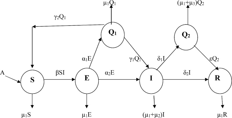
Based on our hypothesis and flow of transmission of the disease COVID-19 in human population as depicted in Fig. 1 , we have the following system of equations:

$$\begin{array}{ccc}\hfill \frac{dS}{dt}& =& A-\beta SI-{\mu }_{1}S+{\gamma }_2{Q}_1\hfill \\ \hfill \frac{dE}{dt}& =& \beta SI-({\alpha }_1+{\alpha }_2+{\mu }_1)E\hfill \\ \hfill \frac{d{Q}_1}{dt}& =& {\alpha }_{1}E-({\gamma }_1+{\gamma }_2+{\mu }_1)Q_1\hfill \\ \hfill \frac{dI}{dt}& =& {\gamma }_1{Q}_1-({\delta }_1+{\delta }_2+{\mu }_1+{\mu }_2)I+{\alpha }_{2}E\hfill \\ \hfill \frac{d{Q}_2}{dt}& =& {\delta }_{1}I-({\mu }_1+{\mu }_3+\epsilon )Q_2\hfill \\ \hfill \frac{dR}{dt}& =& \epsilon Q_2+{\delta }_{2}I-{\mu }_{1}R\hfill \end{array}$$ (1)

Fig. 1.

Schematic diagram of the flow of transmission of COVID-19 in Bhilwara Model.

2.3. Positivity and boundedness of the model

It is assumed that all the population and parameters are nonnegative in the region. So the rate of change of the total population is given by:

$$\begin{array}{ccc}\hfill \frac{dN}{dt}& =& \frac{dS}{dt}+\frac{dE}{dt}+\frac{d{Q}_1}{dt}+\frac{dI}{dt}+\frac{d{Q}_2}{dt}+\frac{dR}{dt}\hfill \\ \hfill \Rightarrow \frac{dN}{dt}& =& A-{\mu }_{1}N-{\mu }_{2}I-{\mu }_3{Q}_2\hfill \end{array}$$

With $N=S+E+Q_1+I+Q_2+R$

It follows that in the absence of the diseases (E = I = Q₂ = 0)

Then $\frac{dN}{dt}=A-{\mu }_{1}N$. This shows that the population size N tends to the carrying capacity $\frac{A}{{\mu }_1}$ as $t\to \infty$.

It follows that the solutions of (1) exists in the region defined by $\Omega =\{(S,E,Q_1,I,Q_2,R)\in R_6^{+}:S\left(t\right)\ge 0,E\left(t\right)\ge 0,Q_1\left(t\right)$ $\ge 0,I\left(t\right)\ge 0,Q_2\left(t\right)\ge 0,R\left(t\right)\ge 0,S+E+Q_1+I+Q_2+R\le \frac{A}{{\mu }_1}\}$Since all the solutions remain bounded in the positively invariant region $\Omega$, the initial value problem is well posed.

2.4. Basic reproduction number (R₀)

In this section, the basic reproduction number of the system (1) will be obtained by the next generation matrix method. The basic reproduction number is defined as the average number of secondary infections when one infective is entered into totally susceptible population. It is denoted as the R₀. This can be calculated as the spectral radius of the FV⁻¹ matrix. This is obtained by linearization of the Eq. (1).

According to the principle of next generation matrix, the basic reproduction number is the spectral radius of the next generation matrix FV⁻¹ of the system of Eq. (1).

Here,

$$f_i-v_i=\left(\begin{array}{c}{\displaystyle \frac{dE}{dt}}\\ {\displaystyle \frac{d{Q}_1}{dt}}\\ {\displaystyle \frac{dI}{dt}}\\ {\displaystyle \frac{d{Q}_2}{dt}}\\ {\displaystyle \frac{dR}{dt}}\end{array}\right)=\left(\begin{array}{c}\beta SI-({\alpha }_1+{\alpha }_2+{\mu }_1)E\\ {\alpha }_{1}E-({\gamma }_1+{\gamma }_2+{\mu }_1)Q_1\\ {\alpha }_{2}E+{\gamma }_1{Q}_1-({\delta }_1+{\delta }_2+{\mu }_1+{\mu }_2)I\\ {\delta }_{1}I-({\mu }_1+{\mu }_3+\epsilon )Q_2\\ \epsilon Q_2+{\delta }_{2}I-{\mu }_{1}R\end{array}\right)$$

Accordingly,

$$f_i=\left(\begin{array}{c}\beta SI\\ 0\\ 0\\ 0\\ 0\end{array}\right),v_i=\left(\begin{array}{c}({\alpha }_1+{\alpha }_2+{\mu }_1)E\\ ({\gamma }_1+{\gamma }_2+{\mu }_1)Q_1-{\alpha }_{1}E\\ ({\delta }_1+{\delta }_2+{\mu }_1+{\mu }_2)I-({\alpha }_{2}E+{\gamma }_1{Q}_1)\\ ({\mu }_1+{\mu }_3+\epsilon )Q_2-{\delta }_{1}I\\ {\mu }_{1}R-(\epsilon Q_2+{\delta }_{2}I)\end{array}\right)$$

here, $f_i$ is the rate of appearance of new infections in compartment i, and $v_i$  is the rate of other transitions between compartment i and other infected compartments, for all $i\in \left[1,5\right]$

The matrix F and V are obtained as follows:

$$F=\left(\begin{array}{ccccc}{\displaystyle \frac{\partial f_1}{\partial E}}& {\displaystyle \frac{\partial f_1}{\partial Q_1}}& {\displaystyle \frac{\partial f_1}{\partial I}}& {\displaystyle \frac{\partial f_1}{\partial Q_2}}& {\displaystyle \frac{\partial f_1}{\partial R}}\\ {\displaystyle \frac{\partial f_2}{\partial E}}& {\displaystyle \frac{\partial f_2}{\partial Q_1}}& {\displaystyle \frac{\partial f_2}{\partial I}}& {\displaystyle \frac{\partial f_2}{\partial Q_2}}& {\displaystyle \frac{\partial f_2}{\partial R}}\\ {\displaystyle \frac{\partial f_3}{\partial E}}& {\displaystyle \frac{\partial f_3}{\partial Q_1}}& {\displaystyle \frac{\partial f_3}{\partial I}}& {\displaystyle \frac{\partial f_3}{\partial Q_2}}& {\displaystyle \frac{\partial f_3}{\partial R}}\\ {\displaystyle \frac{\partial f_4}{\partial E}}& {\displaystyle \frac{\partial f_4}{\partial Q_1}}& {\displaystyle \frac{\partial f_4}{\partial I}}& {\displaystyle \frac{\partial f_4}{\partial Q_2}}& {\displaystyle \frac{\partial f_4}{\partial R}}\\ {\displaystyle \frac{\partial f_5}{\partial E}}& {\displaystyle \frac{\partial f_5}{\partial Q_1}}& {\displaystyle \frac{\partial f_5}{\partial I}}& {\displaystyle \frac{\partial f_5}{\partial Q_2}}& {\displaystyle \frac{\partial f_5}{\partial R}}\end{array}\right)=\left(\begin{array}{ccccc}0& 0& \beta S_0& 0& 0\\ 0& 0& 0& 0& 0\\ 0& 0& 0& 0& 0\\ 0& 0& 0& 0& 0\\ 0& 0& 0& 0& 0\end{array}\right)$$

where ${\displaystyle S_0=\frac{A}{{\mu }_1}}$

And

$$V=\left(\begin{array}{ccccc}{\displaystyle \frac{\partial v_1}{\partial E}}& {\displaystyle \frac{\partial v_1}{\partial Q_1}}& {\displaystyle \frac{\partial v_1}{\partial I}}& {\displaystyle \frac{\partial v_1}{\partial Q_2}}& {\displaystyle \frac{\partial v_1}{\partial R}}\\ {\displaystyle \frac{\partial v_2}{\partial E}}& {\displaystyle \frac{\partial v_2}{\partial Q_1}}& {\displaystyle \frac{\partial v_2}{\partial I}}& {\displaystyle \frac{\partial v_2}{\partial Q_2}}& {\displaystyle \frac{\partial v_2}{\partial R}}\\ {\displaystyle \frac{\partial v_3}{\partial E}}& {\displaystyle \frac{\partial v_3}{\partial Q_1}}& {\displaystyle \frac{\partial v_3}{\partial I}}& {\displaystyle \frac{\partial v_3}{\partial Q_2}}& {\displaystyle \frac{\partial v_3}{\partial R}}\\ {\displaystyle \frac{\partial v_4}{\partial E}}& {\displaystyle \frac{\partial v_4}{\partial Q_1}}& {\displaystyle \frac{\partial v_4}{\partial I}}& {\displaystyle \frac{\partial v_4}{\partial Q_2}}& {\displaystyle \frac{\partial v_4}{\partial R}}\\ {\displaystyle \frac{\partial v_5}{\partial E}}& {\displaystyle \frac{\partial v_5}{\partial Q_1}}& {\displaystyle \frac{\partial v_5}{\partial I}}& {\displaystyle \frac{\partial v_5}{\partial Q_2}}& {\displaystyle \frac{\partial v_5}{\partial R}}\end{array}\right)$$

$$\Rightarrow V=\left(\begin{array}{ccccc}({\alpha }_1+{\alpha }_2+{\mu }_1)& 0& 0& 0& 0\\ -{\alpha }_1& ({\gamma }_1+{\gamma }_2+{\mu }_1)& 0& 0& 0\\ -{\alpha }_2& -{\gamma }_1& ({\delta }_1+{\delta }_2+{\mu }_1+{\mu }_2)& 0& 0\\ 0& 0& -{\delta }_1& ({\mu }_1+{\mu }_3+\epsilon )& 0\\ 0& 0& -{\delta }_2& -\epsilon & {\mu }_1\end{array}\right)$$

Again ${\displaystyle V^{-1}=\frac{AdjV}{\left|V\right|}}$

$$\begin{array}{ccc}& & V^{-1}\hfill \\ & & =\left(\begin{array}{ccccc}{\displaystyle \frac{1}{({\alpha }_1+{\alpha }_2+{\mu }_1)}}& 0& 0& 0& 0\\ {\displaystyle \frac{{\alpha }_1}{({\alpha }_1+{\alpha }_2+{\mu }_1)({\gamma }_1+{\gamma }_2+{\mu }_1)}}& {\displaystyle \frac{1}{({\gamma }_1+{\gamma }_2+{\mu }_1)}}& 0& 0& 0\\ {\displaystyle \frac{{\alpha }_1{\gamma }_1+{\alpha }_2({\gamma }_1+{\gamma }_2+{\mu }_1)}{({\alpha }_1+{\alpha }_2+{\mu }_1)({\gamma }_1+{\gamma }_2+{\mu }_1)({\delta }_1+{\delta }_2+{\mu }_1+{\mu }_2)}}& {\displaystyle \frac{{\gamma }_1}{({\gamma }_1+{\gamma }_2+{\mu }_1)({\delta }_1+{\delta }_2+{\mu }_1+{\mu }_2)}}& {\displaystyle \frac{1}{({\delta }_1+{\delta }_2+{\mu }_1+{\mu }_2)}}& 0& 0\\ {\displaystyle \frac{{\alpha }_2{\delta }_1({\gamma }_1+{\gamma }_2+{\mu }_1)+{\delta }_1{\gamma }_1{\alpha }_1}{({\alpha }_1+{\alpha }_2+{\mu }_1)({\gamma }_1+{\gamma }_2+{\mu }_1)({\delta }_1+{\delta }_2+{\mu }_1+{\mu }_2)({\mu }_1+{\mu }_3+\epsilon )}}& {\displaystyle \frac{{\delta }_1{\gamma }_1}{({\gamma }_1+{\gamma }_2+{\mu }_1)({\delta }_1+{\delta }_2+{\mu }_1+{\mu }_2)({\mu }_1+{\mu }_3+\epsilon )}}& {\displaystyle \frac{-{\delta }_1}{({\delta }_1+{\delta }_2+{\mu }_1+{\mu }_2)({\mu }_1+{\mu }_3+\epsilon )}}& {\displaystyle \frac{-{\delta }_2}{({\delta }_1+{\delta }_2+{\mu }_1+{\mu }_2)({\mu }_1+{\mu }_3+\epsilon )}}& 0\\ \left({\displaystyle \frac{\left(\begin{array}{c}({\mu }_1+{\mu }_3+\epsilon ){\delta }_2{\alpha }_2({\gamma }_1+{\gamma }_2+{\mu }_1)+\epsilon {\delta }_1{\alpha }_1{\gamma }_1\hfill \\ -{\alpha }_1{\delta }_2{\gamma }_1({\mu }_1+{\mu }_3+\epsilon )+({\gamma }_1+{\gamma }_2+{\mu }_1)\epsilon {\delta }_1{\alpha }_2\hfill \end{array}\right)}{({\alpha }_1+{\alpha }_2+{\mu }_1)({\gamma }_1+{\gamma }_2+{\mu }_1)({\delta }_1+{\delta }_2+{\mu }_1+{\mu }_2)({\mu }_1+{\mu }_3+\epsilon ){\mu }_1}}\right)& {\displaystyle \frac{({\mu }_1+{\mu }_3+\epsilon ){\gamma }_1{\delta }_2+{\delta }_1\epsilon {\gamma }_1}{({\gamma }_1+{\gamma }_2+{\mu }_1)({\delta }_1+{\delta }_2+{\mu }_1+{\mu }_2)({\mu }_1+{\mu }_3+\epsilon ){\mu }_1}}& {\displaystyle \frac{{\delta }_2({\mu }_1+{\mu }_3+\epsilon +\epsilon {\delta }_1}{({\delta }_1+{\delta }_2+{\mu }_1+{\mu }_2)({\mu }_1+{\mu }_3+\epsilon ){\mu }_1}}& {\displaystyle \frac{\epsilon }{{\mu }_1}}& {\displaystyle \frac{1}{{\mu }_1}}\end{array}\right)\hfill \end{array}$$

Thus, the basic reproduction number, denoted by Ro is

$$\begin{array}{c}{\displaystyle R_0=\rho \left(F{V}^{-1}\right)=\frac{\beta S_0({\alpha }_1{\gamma }_1+{\alpha }_2({\gamma }_1+{\gamma }_2+{\mu }_1))}{({\alpha }_1+{\alpha }_2+{\mu }_1)({\gamma }_1+{\gamma }_2+{\mu }_1)({\delta }_1+{\delta }_2+{\mu }_1+{\mu }_2)}}\hfill \\ {\displaystyle R_0=\rho \left(F{V}^{-1}\right)=\frac{\beta A({\alpha }_1{\gamma }_1+{\alpha }_2({\gamma }_1+{\gamma }_2+{\mu }_1))}{{\mu }_1({\alpha }_1+{\alpha }_2+{\mu }_1)({\gamma }_1+{\gamma }_2+{\mu }_1)({\delta }_1+{\delta }_2+{\mu }_1+{\mu }_2)}}\hfill \end{array}$$

3. Local and global asymptotic stability

For the steady state conditions, the system of equations (1) becomes

$$\begin{array}{c}A-\beta SI-{\mu }_{1}S+{\gamma }_2{Q}_1=0\hfill \\ \beta SI-({\alpha }_1+{\alpha }_2+{\mu }_1)E=0\hfill \\ {\alpha }_{1}E-({\gamma }_1+{\gamma }_2+{\mu }_1)Q_1=0\hfill \\ {\gamma }_1{Q}_1-({\delta }_1+{\delta }_2+{\mu }_1+{\mu }_2)I+{\alpha }_{2}E=0\hfill \\ {\delta }_{1}I-({\mu }_1+{\mu }_3+\epsilon )Q_2=0\hfill \\ \epsilon Q_2+{\delta }_{2}I-{\mu }_{1}R=0\hfill \end{array}$$ (2)

In this section we discuss the local stability of disease free equilibrium and endemic equilibrium of the system (2) by analyzing the corresponding characteristic equations respectively.

3.1. Stability analysis for diseases-free equilibrium

Theorem 1

If R₀ < 1, the diseases free equilibrium is locally asymptotically stable in the region Ω₀, otherwise it is unstable.

Proof

At the disease free equilibrium ${\Omega }_0(S=1,E=Q_1=I=Q{}_2=0)$, the Jacobian matrix (2) becomes

$$J_{DFE}\left({\Omega }_0\right)=\left(\begin{array}{ccccc}-{\mu }_1& 0& {\gamma }_2& -\beta & 0\\ 0& -({\alpha }_1+{\alpha }_2+{\mu }_1)& 0& \beta & 0\\ 0& {\alpha }_1& -({\gamma }_1+{\gamma }_2+{\mu }_1)& 0& 0\\ 0& 0& {\gamma }_1& -({\delta }_1+{\delta }_2+{\mu }_1+{\mu }_2)& 0\\ 0& 0& 0& {\delta }_1& -(\epsilon +{\mu }_1+{\mu }_3)\end{array}\right)$$

The corresponding eigen values of $J_{DFE}\left({\Omega }_0\right)$ are

$$\begin{array}{c}{\lambda }_1=-{\mu }_1\hfill \\ {\lambda }_2=-(\epsilon +{\mu }_1+{\mu }_3)\hfill \end{array}$$

And other three eigen values can be obtained by solving the cubic polynomial equations

${\lambda }^3+a_1{\lambda }^2+a_2\lambda +a_3=0$, where

$$\begin{array}{c}{a}_1=({\alpha }_1+{\alpha }_2+3{\mu }_1+{\gamma }_1+{\gamma }_2+{\delta }_1+{\delta }_2+{\mu }_2)\hfill \\ a_2=({\alpha }_1+{\alpha }_2+{\mu }_1)({\gamma }_1+{\gamma }_2+{\mu }_1)+({\alpha }_1+{\alpha }_2+{\mu }_1)({\delta }_1+{\delta }_2+{\mu }_1+{\mu }_2)+({\delta }_1+{\delta }_2+{\mu }_1+{\mu }_2)({\gamma }_1+{\gamma }_2+{\mu }_1)\hfill \\ a_3=({\alpha }_1+{\alpha }_2+{\mu }_1)({\gamma }_1+{\gamma }_2+{\mu }_1)({\delta }_1+{\delta }_2+{\mu }_1+{\mu }_2)-\beta {\alpha }_1{\gamma }_1=({\alpha }_1+{\alpha }_2+{\mu }_1)({\gamma }_1+{\gamma }_2+{\mu }_1)({\delta }_1+{\delta }_2+{\mu }_1+{\mu }_2)(1-R_0)\hfill \end{array}$$

If R₀ < 1, we have, a₁ > 0, a₂ > 0, a₃ > 0 and a₁.a₂ > a₃ [21,22].

Numerically, we try to establish the relation

$$a_1>0,a_2>0,a_3>0\text{and}{a}_1·a_2>a_3$$ (3)

For this we refer Example 1 and Table 2 of Section 4 and after substituting the parametric values we establish the relation (3). Details of the calculations may be found in Appendix 1.

Table 2.

Parametric values for the Fig. 2(a)–(e).

Parameter	Values
A	0.02
${\mu }_1$	0.01
${\mu }_2$	0.018
${\mu }_3$	0.015
$\beta$	0.1
${\alpha }_1$	0.3
${\alpha }_2$	0.05
${\gamma }_1$	0.3
${\gamma }_2$	0.02
${\delta }_1$	0.07
${\delta }_2$	0.1
$\epsilon$	0.02
$\left(S_0,E_0,Q_{1_0},I_0,Q_{2_0},R_0\right)$	(0.69, 0.27, 0.0, 0.03, 0.01, 0.0)
$\left(R_0<1\right),R_0=$	0.90551984491

Thus by Routh-Hurwitz criterion, if R₀ < 1, $J_{DFE}\left({\Omega }_0\right)$is locally asymptotically stable in the region.

3.2. Endemic equilibrium

The endemic equilibrium ${\Omega }^{*}(S^{*},E^{*},Q_1^{*},I^{*},Q_2^{*},R^{*})$, can be obtained by solving the Eq. (2) simultaneously, we have,

$$\begin{array}{c}{\displaystyle S^{*}=\frac{A{R}_0{\gamma }_1-(\beta {\gamma }_1+R_0({\mu }_1+{\mu }_2+{\delta }_1+{\delta }_2))I^{*}}{R_0{\mu }_1{\gamma }_1}}\hfill \\ {\displaystyle E^{*}=\frac{\beta I^{*}}{R_0({\alpha }_1+{\alpha }_2+{\mu }_1)}}\hfill \\ {\displaystyle Q_1^{*}=\frac{({\mu }_1+{\mu }_2+{\delta }_1+{\delta }_2))I^{*}}{{\gamma }_1}}\hfill \\ {\displaystyle I^{*}=\frac{{\gamma }_1{Q}_1^{*}}{({\mu }_1+{\mu }_2+{\delta }_1+{\delta }_2)}}\hfill \\ {\displaystyle Q_2^{*}=\frac{{\delta }_1{I}^{*}}{(\epsilon +{\mu }_1+{\mu }_3)}}\hfill \\ {\displaystyle R^{*}=\frac{(\epsilon {\delta }_1+{\delta }_2(\epsilon +{\mu }_1+{\mu }_3))I^{*}}{{\mu }_1(\epsilon +{\mu }_1+{\mu }_3)}}\hfill \end{array}$$

3.2.1. Local stability of endemic equilibrium

Theorem 2

The endemic equilibrium ${\Omega }^{*}(S^{*},E^{*},Q_1^{*},I^{*},Q_2^{*},R^{*})$ is locally asymptotically stable when R₀ > 1, otherwise it is unstable.

Proof

At the endemic equilibrium${\Omega }^{*}(S^{*},E^{*},Q_1^{*},I^{*},Q_2^{*},R^{*})$, the Variation matrix (2) becomes

$${{\Omega }_{EE}}^{*}(S^{*},E^{*},Q_1^{*},I^{*},Q_2^{*},R^{*})=\left(\begin{array}{cccccc}-(\beta I^{*}+{\mu }_1)& 0& {\gamma }_2& -\beta S^{*}& 0& 0\\ \beta I^{*}& -({\alpha }_1+{\alpha }_2+{\mu }_1)& 0& \beta S^{*}& 0& 0\\ 0& {\alpha }_1& -({\gamma }_1+{\gamma }_2+{\mu }_1)& 0& 0& 0\\ 0& 0& {\gamma }_1& -({\delta }_1+{\delta }_2+{\mu }_1+{\mu }_2)& 0& 0\\ 0& 0& 0& {\delta }_1& -(\epsilon +{\mu }_1+{\mu }_2)& 0\\ 0& 0& 0& {\delta }_2& \epsilon & -{\mu }_1\end{array}\right)$$

The corresponding eigen values are

$$\begin{array}{c}{\lambda }_1=-{\mu }_1\hfill \\ {\lambda }_2=-(\epsilon +{\mu }_1+{\mu }_2)\hfill \end{array}$$

And other four eigen values can be obtained by solving the forth degree polynomial equations

${\lambda }^4+A_1{\lambda }^3+A_2{\lambda }^2+A_3\lambda +A_4=0$, where

$$\begin{array}{c}{A}_1=(\beta I^{*}+{\alpha }_1+{\alpha }_2+{\gamma }_1+{\gamma }_2+{\delta }_1+{\delta }_2+4{\mu }_1+{\mu }_2)\hfill \\ A{}_2=\left(\begin{array}{c}(\beta I^{*}+{\mu }_1)({\alpha }_1+{\alpha }_2+{\mu }_1)+(\beta I^{*}+{\mu }_1)({\delta }_1+{\delta }_2+{\mu }_1+{\mu }_2)+({\gamma }_1+{\gamma }_2+{\mu }_1)(\beta I^{*}+{\mu }_1)\hfill \\ +({\alpha }_1+{\alpha }_2+{\mu }_1)({\delta }_1+{\delta }_2+{\mu }_1+{\mu }_2)+({\alpha }_1+{\alpha }_2+{\mu }_1)({\gamma }_1+{\gamma }_2+{\mu }_1)+({\gamma }_1+{\gamma }_2+{\mu }_1)({\delta }_1+{\delta }_2+{\mu }_1+{\mu }_2)\hfill \end{array}\right)\hfill \\ A_3=\left(\begin{array}{c}(\beta I^{*}+{\mu }_1)({\alpha }_1+{\alpha }_2+{\mu }_1)({\delta }_1+{\delta }_2+{\mu }_1+{\mu }_2)+(\beta I^{*}+{\mu }_1)({\alpha }_1+{\alpha }_2+{\mu }_1)({\gamma }_1+{\gamma }_2+{\mu }_1)\hfill \\ +(\beta I^{*}+{\mu }_1)({\gamma }_1+{\gamma }_2+{\mu }_1)({\delta }_1+{\delta }_2+{\mu }_1+{\mu }_2)+({\gamma }_1+{\gamma }_2+{\mu }_1)({\delta }_1+{\delta }_2+{\mu }_1+{\mu }_2)({\alpha }_1+{\alpha }_2+{\mu }_1)-\beta I^{*}{\alpha }_1{\gamma }_2-\beta S^{*}{\gamma }_1{\alpha }_1\hfill \end{array}\right)\hfill \\ A_4=\left((\beta I^{*}+{\mu }_1)({\alpha }_1+{\alpha }_2+{\mu }_1)({\delta }_1+{\delta }_2+{\mu }_1+{\mu }_2)({\gamma }_1+{\gamma }_2+{\mu }_1)-(\beta I^{*}+{\mu }_1)\beta S^{*}{\gamma }_1{\alpha }_1+{\beta }^2{S}^{*}{I}^{*}{\alpha }_1{\gamma }_1-\beta I^{*}{\gamma }_2{\alpha }_1({\delta }_1+{\delta }_2+{\mu }_1+{\mu }_2)\right)\hfill \end{array}$$

Since here,

$$\begin{array}{c}{A}_1>0,A_3>0,A_4>0\hfill \\ A_1{A}_2{A}_3>A_3^2+A_1^2{A}_4\hfill \\ \Rightarrow A_1{A}_2{A}_3-(A_3^2+A_1^2{A}_4)>0\hfill \end{array}$$

To establish the relation

$$A_1>0,A_3>0,A_4>0\text{and}\begin{array}{c}{A}_1{A}_2{A}_3>A_3^2+A_1^2{A}_4\\ \Rightarrow A_1{A}_2{A}_3-(A_3^2+A_1^2{A}_4)>0\end{array}$$ (4)

we refer Example 2 and Table 3 (at equilibrium point $I^{*}=0.057$and $S^{*}=0.6149$) and Table 4 of Section 4. Numerically, the relation (4) holds. The details of calculation may be found in Appendix 2.

Table 3.

Time series for Fig. 3(a).

Time	S	E	Q1	I	Q2	R
0	0.6900	0.2700	0	0.0300	0.0100	0
0.0303	0.6901	0.2673	0.0024	0.0302	0.0100	0
1.0270	0.6937	0.1953	0.0595	0.0446	0.0121	0.0039
4.2489	0.6744	0.1039	0.0975	0.1038	0.0265	0.0291
9.0555	0.5949	0.0930	0.0881	0.1401	0.0597	0.0910
16.6718	0.4816	0.0843	0.0807	0.1473	0.1085	0.2042
29.4431	0.4012	0.0576	0.0578	0.1179	0.1520	0.3738
44.5427	0.4218	0.0382	0.0374	0.0768	0.1488	0.4983
58.0234	0.4805	0.0313	0.0295	0.0573	0.1270	0.5530
64.9592	0.5134	0.0301	0.0278	0.0524	0.1157	0.5688
72.4715	0.5468	0.0301	0.0273	0.0499	0.1052	0.5804
92.6840	0.6073	0.0349	0.0308	0.0532	0.0896	0.6018
100	0.6149	0.0378	0.0332	0.0570	0.0885	0.6108

Table 4.

Parameter values for the Fig. 3(a), 3(b), 3(c), 3(d), 3(e) and 3(f).

Parameter	Values
A	0.02
${\mu }_1$	0.02
${\mu }_2$	0.03
${\mu }_3$	0.035
$\beta$	0.4
${\alpha }_1$	0.3
${\alpha }_2$	0.05
${\gamma }_1$	0.3
${\gamma }_2$	0.02
${\delta }_1$	0.07
${\delta }_2$	0.1
$\epsilon$	0.02
$\left(S_0,E_0,Q_{1_0},I_0,Q_{2_0},R_0\right)$	(0.69, 0.27, 0.0, 0.03, 0.01, 0.0)
$\left(R_0>1\right),R_0=$	3.62207937965

So, by Routh-Hurwitz criterion, if R₀ > 1, then the endemic equilibrium is locally asymptotically stable.

3.2.2. Global stability for endemic equilibrium

In this section we will derive the global stability of endemic equilibrium using Poincare Bendixson technique [23].

Let us define a mapping $f\left(x\right):D\subset R^n\to R^n$, where D is an open set, if the differential equation $I^{/}=f\left(x\right)$ be such that its every solution x(t) can be uniquely determined by its initial conditions x(t) = x₀, then an equilibrium point $\overline{x}\in D$, and satisfies some conditions:

• (1)D is simply connected.
• (2)There exists a compact absorbing subset Kof D.
• (3) $\overline{x}$ is the only equilibrium point in D is globally stable if it satisfies the additional Bendixson condition given by ${\overline{q}}_2=\lim \underset{t\to \infty }{sup}\underset{x_0\in K}{sup}q<0$

where $q=\underset{o}{\overset{t}{\int }}\psi \left(Z\left(x(s,x_0)\right)\right)ds$.

Also $Z=P_f{P}^{-1}+P\frac{\partial f^{\left[2\right]}}{\partial x}{P}^{-1}$ and P be the matrix valued function satisfying $\psi (P_f{P}^{-1}+P{J}^{\left[2\right]}{P}^{-1})\le 0$ on K. Again $J^{\left[2\right]}=\frac{\partial f^{\left[2\right]}}{\partial x}$ is the second compound additive Jacobian matrix of order 4 and Ψ be the Lozinskii measure given by a formula $\psi \left(M\right)=\underset{h\to 0^{+}}{lim}\frac{\left|I+hM\right|-1}{h}$ for n by n matrix M.

The existence of a compact absorbing set which is absorbing in the interior of Ω. It follows from the uniform persistence of the system as $\lim \underset{t\to \infty }{inf}S\left(t\right)\ge C$,$\lim \underset{t\to \infty }{inf}E\left(t\right)\ge C$,$\lim \underset{t\to \infty }{inf}{Q}_1\left(t\right)\ge C$,$\lim \underset{t\to \infty }{inf}I\left(t\right)\ge C$,$\lim \underset{t\to \infty }{inf}{Q}_2\left(t\right)\ge C$,$\lim \underset{t\to \infty }{inf}R\left(t\right)\ge C$ for some C>0. According to this procedure we discuss geometric approach of Li and Muldowney [24] to the global stability of the region Ω .

Theorem 3

If R₀ > 1 then the system (2) is globally asymptotically stable in the region Ω.

Proof

The Jacobian matrix of reduced system(2), leaving the exposed and recovered populations

$$J=\left(\begin{array}{cccc}-({\mu }_1+\beta I)& -\beta S& {\gamma }_2& 0\\ 0& -({\mu }_1+{\mu }_2+{\delta }_1+{\delta }_2)& {\gamma }_1& 0\\ 0& 0& -({\mu }_1+{\gamma }_1+{\gamma }_2)& 0\\ 0& {\delta }_1& 0& -({\mu }_3+\epsilon +{\mu }_1)\end{array}\right)$$

As we know that the second additive compound matrix of A=(a_ij) of order 4 is

$$A^{\left[2\right]}=\left(\begin{array}{cccccc}{a}_{11}+a_{22}& a_{23}& a_{24}& -a_{13}& -a_{14}& 0\\ 0& a_{11}+a_{33}& a_{34}& a_{12}& 0& -a_{14}\\ a_{42}& a_{43}& a_{11}+a_{44}& 0& a_{12}& a_{13}\\ -a_{31}& a_{21}& 0& a_{22}+a_{33}& a_{34}& -a_{24}\\ a_{41}& 0& a_{21}& a_{43}& a_{22}+a_{44}& a_{23}\\ 0& -a_{41}& a_{31}& -a_{42}& a_{32}& a_{33}+a_{44}\end{array}\right)$$

Therefore, the second additive compound matrix of J ($J^{\left[2\right]}$) of order 4 is calculated as

$$J^{\left[2\right]}=\left(\begin{array}{cccccc}-(2{\mu }_1+\beta I+{\mu }_2+{\delta }_1+{\delta }_2)& {\gamma }_1& 0& -{\gamma }_2& 0& 0\\ 0& -(2{\mu }_1+\beta I+{\gamma }_1+{\gamma }_2)& 0& -\beta S& 0& 0\\ {\delta }_1& 0& -(2{\mu }_1+\beta I+{\mu }_3+\epsilon )& 0& -\beta S& {\gamma }_2\\ 0& 0& 0& -(2{\mu }_1+{\mu }_2+{\delta }_1+{\delta }_2+{\gamma }_1+{\gamma }_2)& 0& 0\\ 0& 0& 0& {\delta }_1& -(2{\mu }_1+{\mu }_2+{\delta }_1+{\delta }_2+{\mu }_3+\epsilon )& {\gamma }_1\\ 0& 0& 0& -{\delta }_1& 0& -(2{\mu }_1+{\mu }_3+\epsilon +{\gamma }_1+{\gamma }_2)\end{array}\right)$$

For finding the matrix Z in the Bendixson criteria, we define a diagonal matrix P as

$$P=daig\left\{{\displaystyle 1,\frac{I}{Q_1},\frac{I}{Q_1},\frac{I}{Q_1},\frac{I}{Q_1},\frac{I}{Q_1}}\right\}$$

Also if f be the vector field of the system then

$$P_f{P}^{-1}=diag\left\{{\displaystyle 0,\frac{I^{/}}{I}-\frac{Q_1^{/}}{Q_1},\frac{I^{/}}{I}-\frac{Q_1^{/}}{Q_1},\frac{I^{/}}{I}-\frac{Q_1^{/}}{Q_1},\frac{I^{/}}{I}-\frac{Q_1^{/}}{Q_1},\frac{I^{/}}{I}-\frac{Q_1^{/}}{Q_1}}\right\}$$

Hence the matrix Z is given by $Z=P_f{P}^{-1}+P{J}^{\left[2\right]}{P}^{-1}=\left(\begin{array}{cc}{Z}_{11}& Z_{12}\\ Z_{21}& Z_{22}\end{array}\right)$

$$Z=\left(\begin{array}{cccccc}-(2{\mu }_1+\beta I+{\mu }_2+{\delta }_1+{\delta }_2)& {\displaystyle \frac{{\gamma }_1{Q}_1}{I}}& 0& {\displaystyle -\frac{{\gamma }_2{Q}_1}{I}}& 0& 0\\ 0& -(2{\mu }_1+\beta I+{\gamma }_1+{\gamma }_2)+Y& 0& -\beta S& 0& 0\\ {\displaystyle \frac{{\delta }_{1}I}{Q_1}}& 0& -(2{\mu }_1+\beta I+{\mu }_3+\epsilon )+Y& 0& -\beta S& {\gamma }_2\\ 0& 0& 0& -(2{\mu }_1+{\mu }_2+{\delta }_1+{\delta }_2+{\gamma }_1+{\gamma }_2)+Y& 0& 0\\ 0& 0& 0& {\delta }_1& -(2{\mu }_1+{\mu }_2+{\delta }_1+{\delta }_2+{\mu }_3+\epsilon )+Y& {\gamma }_1\\ 0& 0& 0& -{\delta }_1& 0& -(2{\mu }_1+{\mu }_3+\epsilon +{\gamma }_1+{\gamma }_2)+Y\end{array}\right)$$

where ${\displaystyle Y=\frac{I^{/}}{I}-\frac{Q_1^{/}}{Q_1}}$

Therefore the block matrix can be written as $Z=\left(\begin{array}{cc}{Z}_{11}& Z_{12}\\ Z_{21}& Z_{22}\end{array}\right)$where

$$\begin{array}{c}{Z}_{11}=(-(2{\mu }_1+\beta I+{\mu }_2+{\delta }_1+{\delta }_2))\hfill \\ Z_{12}=\left(\begin{array}{ccccc}{\displaystyle \frac{{\gamma }_1{Q}_1}{I}}& 0& {\displaystyle \frac{{\gamma }_2{Q}_1}{I}}& 0& 0\end{array}\right)\hfill \\ Z_{21}=\left(\begin{array}{c}0\\ {\displaystyle \frac{{\delta }_{1}I}{Q_1}}\\ 0\\ 0\\ 0\end{array}\right)\hfill \end{array}$$

$$Z_{22}=\left(\begin{array}{ccccc}-(2{\mu }_1+\beta I+{\gamma }_1+{\gamma }_2)+Y& 0& -\beta S& 0& 0\\ 0& -(2{\mu }_1+\beta I+{\mu }_3+\epsilon )+Y& 0& -\beta S& {\gamma }_2\\ 0& 0& -(2{\mu }_1+{\mu }_2+{\delta }_1+{\delta }_2+{\gamma }_1+{\gamma }_2)+Y& 0& 0\\ 0& 0& {\delta }_1& -(2{\mu }_1+{\mu }_2+{\delta }_1+{\delta }_2+{\mu }_3+\epsilon )+Y& {\gamma }_1\\ 0& 0& -{\delta }_1& 0& -(2{\mu }_1+{\mu }_3+\epsilon +{\gamma }_1+{\gamma }_2)+Y\end{array}\right)$$

The Lozinskii measure of matrix Z can be estimated as $\psi \left(Z\right)\le \sup \left\{k_1,k_2\right\}$, where k₁, k₂ defined as

$$\begin{array}{c}{k}_1=\psi \left(Z_{11}\right)+\left|Z_{12}\right|\hfill \\ k_2=\left|Z_{21}\right|+\psi \left(Z_{22}\right)\hfill \end{array}$$

Hence k₁ and k₂ is reduced to

$$\begin{array}{c}{\displaystyle k_1=\psi \left(Z_{11}\right)+\left|Z_{12}\right|=-(2{\mu }_1+\beta I+{\mu }_2+{\delta }_1+{\delta }_2)+\frac{{\gamma }_1{Q}_1}{I}\le \frac{I^{/}}{I}-{\mu }_1}\hfill \\ {\displaystyle k_2=\left|Z_{21}\right|+\psi \left(Z_{22}\right)=\frac{{\delta }_{1}I}{Q_1}-(2{\mu }_1+{\mu }_2+{\delta }_1+{\delta }_2+{\gamma }_1+{\gamma }_2)+Y\le \frac{I^{/}}{I}-\mu }\hfill \end{array}$$

So $\psi \left(Z\right)\le \frac{I^{/}}{I}-{\mu }_1$

Hence $\underset{0}{\overset{t}{\int }}\psi \left(Z\right)dt<(\log I\left(t\right)-{\mu }_{1}t)$

Therefore finally we obtain $\stackrel{-}{q_2}=\frac{\underset{0}{\overset{t}{\int }}\psi \left(Z\right)dt}{t}<\frac{\log I\left(t\right)}{t}-{\mu }_1<0$, for all $(S\left(0\right),E\left(0\right),Q_1\left(0\right),I\left(0\right),Q_2\left(0\right),R\left(0\right))$ in the absorbing set, where the bound on the sizes of the populations are implied by the uniform persistence of the system . The criteria $\stackrel{-}{q_2}<0$ is thus satisfied and so the endemic equilibrium is globally stable. This condition itself proves the global stability of unique positive equilibrium in the region. This completes the proof. Number of authors has used a similar approach to prove this theorem [25,26].

4. Simulation and analysis

In this section, some experiments have been performed to verify analytically obtained results. Simulations have been carried out for Bhilwara model to depict local and global stability. Some examples are mentioned below for simulating the models either for $R_o<1$or for$R_o>1$.

Example 1

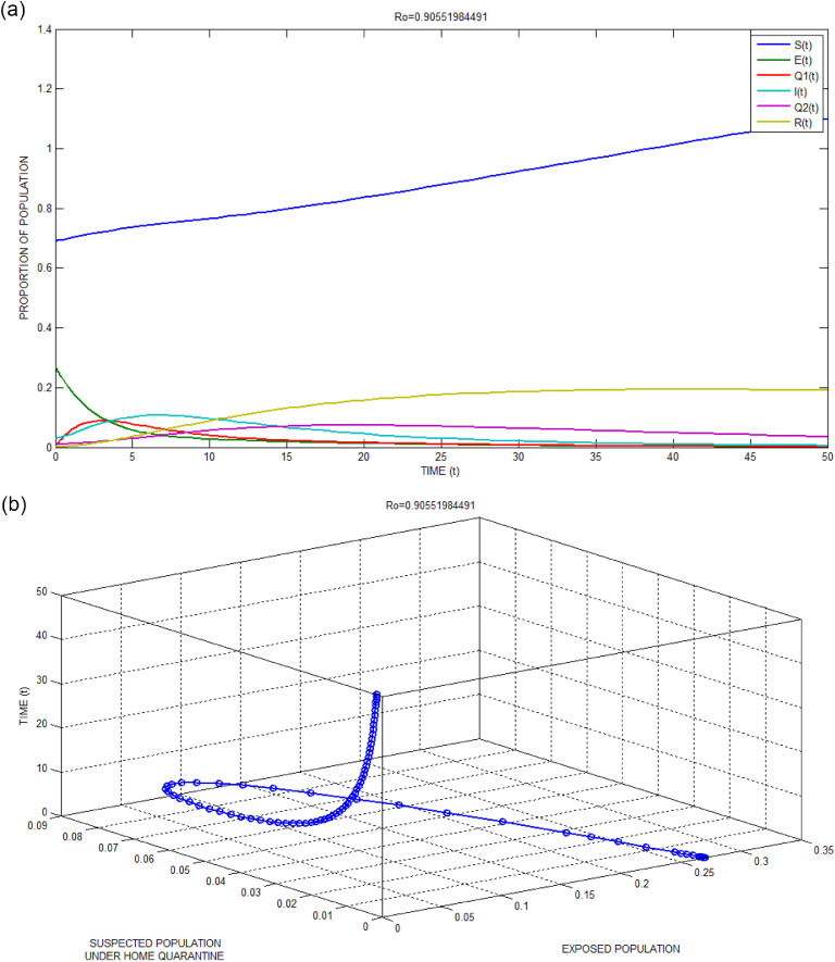
The local stability of the infection-free equilibrium point has been numerically simulated and depicted in Fig. 2 (a) and the corresponding simulated data for this unsuccessful attack are listed in Table 1 . The initial point and the parametric values along with basic reproduction number $\left(R_o\right)$are shown in Table 2 . The value of $R_o$is obtained as less than one. It is clearly observed that the infection-free equilibrium point turns out to be stable for all the stages.

Fig. 2.

(a): Local stability of infection-free equilibrium for Bhilwara Model when $R_0<1$

(b): Exposed Population versus Suspected Population with respect to time for Bhilwara Model when$R_0<1$.

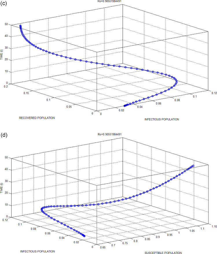
(c): Infectious Population versus Recovered Population with respect to time for Bhilwara Model when$R_0<1$.

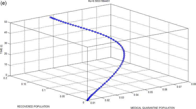
(d): Susceptible Population versus Infectious Population with respect to time for Bhilwara Model when$R_0<1$.

(e): Medical Quarantine Population versus Recovered Population with respect to time for Bhilwara Model when$R_0<1$.

Table 1.

Time series for Fig. 2(a).

Time	S	E	Q1	I	Q2	R
0	0.6900	0.2700	0	0.0300	0.0100	0
0.0303	0.6903	0.2671	0.0024	0.0302	0.0100	0
1.0255	0.7014	0.1888	0.0586	0.0444	0.0121	0.0039
4.2264	0.7310	0.0703	0.0842	0.0961	0.0258	0.0279
8.9068	0.7593	0.0307	0.0470	0.1014	0.0517	0.0780
15.1168	0.7986	0.0184	0.0233	0.0667	0.0708	0.1315
24.0367	0.8704	0.0098	0.0114	0.0327	0.0713	0.1732
34.7309	0.9659	0.0048	0.0054	0.01476	0.0570	0.1913
50	1.1001	0.0019	0.0021	0.0054	0.0354	0.1900

Bhilwara city, the first epicentre in India during COVID-19 outbreak, not only controlled the spread of this coronavirus but also made the city corona free. Along with a curfew(just like lockdown), an extensive door to door survey were conducted for possible identification of individuals suffering from influenza-like illness symptoms and were kept in home quarantine. The same fact is incorporated in our model using very high value for$\left({\alpha }_1\right)$, the rate of transfer of exposed population (E) to suspected population under home quarantine (Q₁). It helps to maintain a low value for$\left(\beta \right)$, per infectivity contact rate by removing the possibly infected population from the mass. Further proper screening and testing for Q₁ helped to detect COVID-19 positive infectious cases (I) to finally move them to medical quarantine compartment (Q₂). This task is also performed fast and the same is considered in our simulation with a higher value for $\left({\gamma }_1\right)$. Rapid identification of positive cases helped early contact tracing and play a vital role to mitigate the spread of coronavirus. The same is experienced here for $R_o$< 1 and from Fig. 2(a) it is clearly observed that the infection will die out in the due course of time.

Example 2

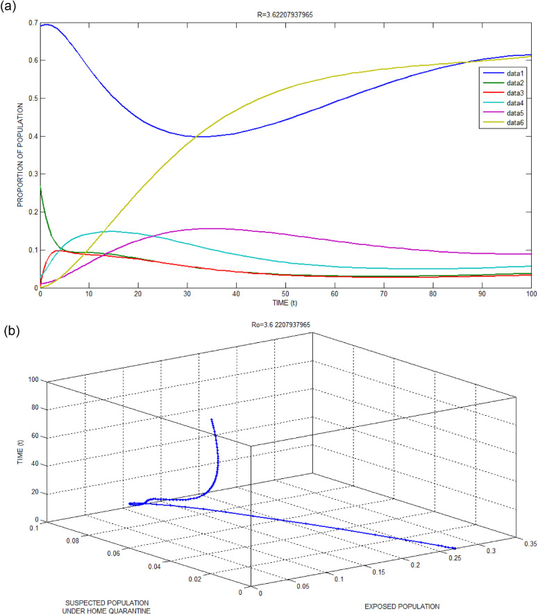
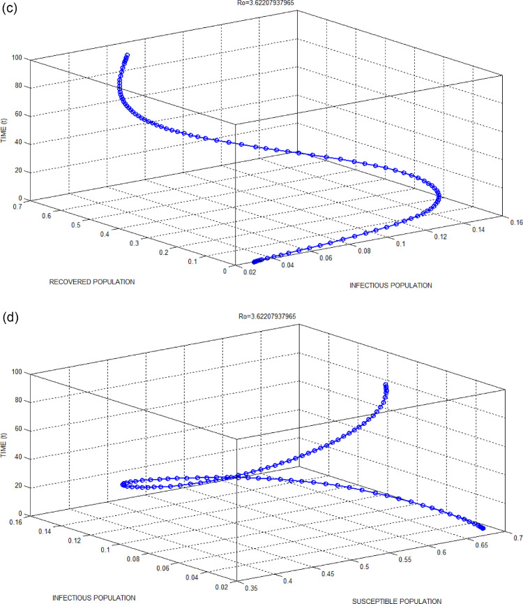
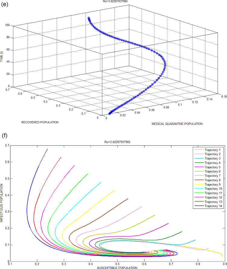
The local stability of the endemic equilibrium point has been numerically simulated and depicted in Fig. 3 (a) and the corresponding simulated data for this successful attack are listed in Table 3 . The initial point and the parametric values along with basic reproduction number $\left(R_o\right)$are shown in Table 4 . The value of $R_o$is obtained as greater than one. It is clearly observed that the endemic equilibrium point turns out to be stable for all the stages. In the absence of lockdown, the per infectivity contact rate$\left(\beta \right)$is obviously very high which make this a successful attack for $R_o>0$.

Fig. 3.

(a): Local stability of infection-endemic equilibrium for Bhilwara Model when$R_0>1$.

(b): Exposed Population versus Suspected Population with respect to time for Bhilwara Model when$R_0>1$.

(c): Infectious Population versus Recovered Population with respect to time for Bhilwara Model when$R_0>1$.

(d): Susceptible Population versus Infectious Population with respect to time for Bhilwara Model when$R_0>1$.

(e): Medical Quarantine Population versus Recovered Population with respect to time for Bhilwara Model when$R_0>1$.

(f): Global stability of infection-endemic equilibrium shown in S-I phase plane for $R_0>1$.

Example 3

The behaviour of system 1 is studied by considering the following with respect to time for $R_o<1$ and $R_o>1$:

• 1)Exposed population verses suspected population
• 2)Infectious population verses recovered population
• 3)Susceptible population verses infectious population and
• 4)Medical quarantine population verses recovered population.

Figs. 2(b) and 3(b) show the favourable situation where exposed populations are quickly surveyed and converted to suspected population if influenza-like illness symptoms present. This quick survey goes in vain for 3(b) as the infectivity contact rate is very high due to no restriction in people’s movement through lockdown.

Figs. 2(c) and 3(c) show a large number of infected populations are recovered. Especially for India where 65percent population are less than 35 years, the recovery is very high. Similarly, Figs. 2(e) and 3(e) show that most of the medical quarantine population are also recovered with time.

Fig. 2(d) clearly shows the advantage of home quarantine compartment. When $\left(R_o<1\right)$, susceptible population moves to home quarantine which reduces$\left(\beta \right)$and as a result less number of people get infected to COVID-19. Whereas, in Fig. 3(d), as large number of people ignores curfew (lockdown), the infectivity contact rate increases $\left(\beta \right)$ and as a result number of infected population increases.

Example 4

The global stability of the endemic equilibrium point for$R_o>1$ is shown in Fig. 3(f). It shows the plane formed by the susceptible population and infectious population. It can be clearly seen from the Fig. 3(e) that the trajectories are seen to asymptotically approach the stable endemic equilibrium point which is unique and globally stable.

5. Impact of lockdown, forecasting and statistical analysis

The different phases of lockdown in India and its impact, that is, active cases, death due to corona virus is mentioned in Table 5 .

Table 5.

The impact of corona virus during the different phases of lockdown in India.

S. No.	Lockdown	Total number of Active Cases		Total number of Deaths
		Start	End	Start	End
1.	Phase 1 (25/03/2020 to 14/04/2020)	606	10,815	10	353
2.	Phase 2 (15/04/2020 to 03/05/2020)	11,933	40,263	392	1306
3.	Phase 3 (04/05/2020 to 17/05/2020)	42,836	90,927	1389	2872
4.	Phase 4 (18/05/2020 to 31/05/2020)	96,169	1,82,143	3029	5164
5.	Unlock 01 (01/06/2020 to 04/06/2020)	1,90,535	2,16,919	5394	6075

5.1. Description and measures taken during different lockdown phases in India

Phase 1 (25^th March to 14^th April)

On 25th March, the first day of the lockdown, nearly all services and factories were suspended. Government took strict measures for those violating norms of lockdown, government took various measures in the form of allocation of funds to mitigate the economic impacts of the lockdown.

Flight operations were suspended for defined time period. Based on regular follow-up lockdown phase was extended till the end of April. At the end of the initial period, the rate of growth of COVID infections had significantly slowed, from a rate of doubling every three days prior to the lockdown to one of doubling every eight days.

Phase II (15^th April to 3^rd May)

On 14 April, Government made lockdown measures strict and ensured aggressive monitoring of the infections. On 16 April, lockdown areas were classified based on the severity in terms of the number of cases for example "red zone" area indicating the presence of infection hotspots, "orange zone" area indicating some infection, and "green zone" area with no infections.

The government announced certain relaxations from 20 April to some industry sectors such as agricultural businesses, Public works programmes with instructions to maintain social distancing. Cargo transportation vehicles and Banks and government centres were also opened.

New guidelines on screening the people, quarantine them and to do periodic health check-ups were strictly implemented.

Phase III (4^th May to 17^th May)

On 1 May, the Ministry of Home Affairs (MHA) and the Government of India further extended the lockdown period to two weeks beyond 4 May, with some relaxations. India has been split into 3 zones: red zones (130 districts), orange zones (284 districts) and green zones (319 districts). Red zones are those with high coronavirus cases and a high doubling rate, orange zones are those with comparatively fewer cases and green zones are those without any cases in the past 21 days. Normal movement was permitted in green zones with buses limited to 50 percent capacity. Orange zones allowed only private and hired vehicles but no public transportation. The red zones remained under lockdown. It was decided to ensure revision of zone classification once a week.

Phase IV (18^th May to 31^st May)

On 17 May, the National Disaster Management Authority (NDMA) and the Ministry of Home Affairs (MHA) extended the lockdown for a period for two weeks beyond 18 May, with additional relaxations. Red zone areas were further divided into containment and buffer zones in order to facilitate and focus the problem areas better with appropriate resource allocation and planning of relief from crisis.

The above descriptions also highlight various key initiatives taken by government agencies and NGO bodies to fight with the epidemic. The strategy of classifying the zones based on number of infected cases proved to be a very effective one as it facilitated in focusing danger zones and accordingly plan and implement corrective measures were initiated.

5.2. Comparative trend analysis of COVID- 19 infected cases during the lockdown periods in different part of the world

5.2.1. Statistical analysis between India (during lockdown in India) and other nations of the world

Non-parametric test is used to assess whether there is significant difference in the infected cases between India (during lockdown in India) and other nations of the world.

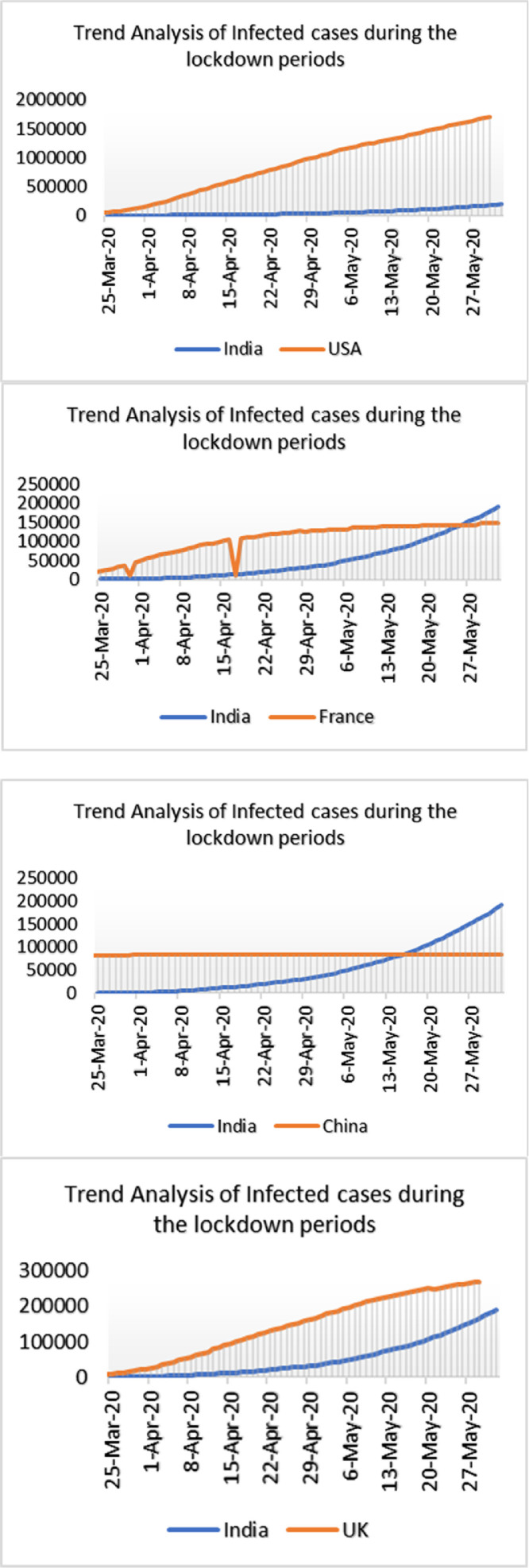
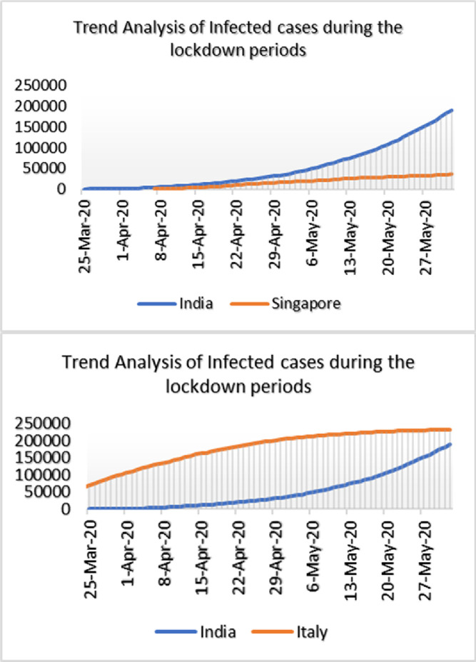
Statistical Analysis using SPSS has been performed to analyse the impact of lockdown in different part of the world badly infected by COVID-19 with India which is depicted in Fig. 4 . It is observed that the countries which implemented lockdown effectively, the infection rate was comparatively less. Non-parametric significance test (Mann Whitney test) was performed using SPSS at 95% and 99% level of significance of infected cases during the lockdown phases between India and other nations of the world and the result is observed in Table 6 .

Fig. 4.

Trend analysis of infected cases during lockdown period of different parts of the world badly infected by COVID-19 having Comparative Assessment with India.

Table 6.

Test of significance of infected cases during the lockdown phases between India and other nations of the world.

Countries compared	Non-Parametric Mann Whitney U value	Z-Score	P Value	Significance at p < 0.05	Significance at p < 0.01
India Vs Singapore	1446	2.41033	.01596	significant	not significant
India Vs France	1488	-2.87373	.0041	significant	Significant
India Vs Italy	839	7.60431	< .00001	significant	Significant
India Vs USA	605	-6.75425	< .00001	significant	Significant
India Vs China	2124	2.19881	0.0278	significant	not significant

Data studied: Number of infected cases of COVID 19 in India and other nations during the lockdown phases of India starting March to May 2020.

Null Hypothesis: There is no statistically significant difference in the number of infected cases during lock down phases between India and other nations of the world.

Alternate Hypothesis: There is statistically significant difference in the number of infected cases during lock down phases between India and other nations of the world.

Discussion: Non-Parametric Mann Whitney test was performed to test the null hypothesis. The results presented in Table 6 indicate that there is a significant difference in the number of infected cases during lockdown phase between India and other countries at 95% confidence interval. The infected cases are not significant at 99% confidence interval for India versus Singapore and India versus China.

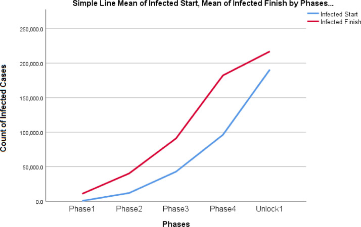
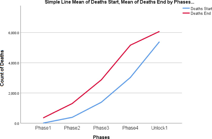
Figs. 5 and 6 represent an increasing trend for both infected cases of COVID- 19 at the start of Lockdown phase and at the end of the Lockdown phases. The infected cases and deaths are not statistically significant between the phase 1 and phase 2, phase 2 & phase 3, phase 3 & phase 4 and phase 4 and Unlock phase 1 at 99% confidence interval.

Fig. 5.

Trend analysis for infected cases during the start and end of the lockdown phases in India

Fig. 6.

Trend analysis for deaths during the start and end of the lockdown phases in India

We then performed continent wise Statistical analysis using Nonparametric Mann Whitney Test. Under this test we observed that null hypothesis is rejected and there is statistically significant difference identified between the infected cases and the deaths when compared between Asia and other continents (Table 7 ).

Table 7.

Continent wise statistical analysis using nonparametric Mann Whitney test.

Comparison between continents	Cases	Deaths	Remarks for Cases	Remarks for Deaths
Asia Vs Others	p < 0.05	p < 0.05	Statistically significant	Statistically significant
Asia Vs Europe	p = 0.027	p < 0.06	Statistically significant	Statistically significant
Asia Vs America	p < 0.05	p = 0.188	Statistically significant	Statistically significant
Asia Vs Africa	p < 0.05	p < 0.05	Statistically significant	Statistically significant
Asia Vs Oceania	p < 0.05	p < 0.05	Statistically significant	Statistically significant

5.2.2. Statistical analysis between different continents of the world

Non-parametric test is used to assess whether there is significant difference in the number of cases due to COVID-19 between the different continents.

Data studied: The data studied under this scenario includes number of infected cases of COVID 19 from different continents. The Asian continent is compared against the remaining continents as depicted in Figs. 7 to 10.

Fig. 7.

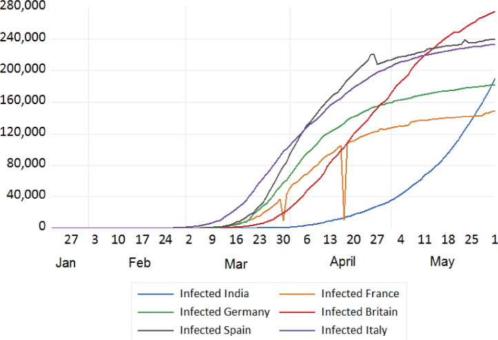
Trend analysis of cumulative infected cases of India and European Countries.

Fig. 10.

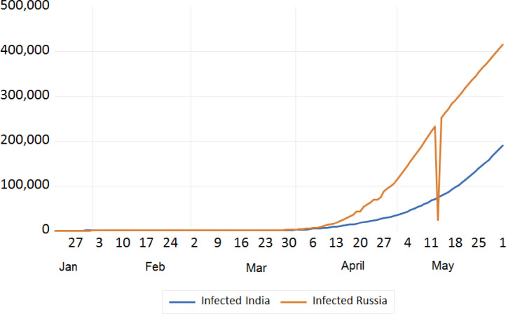
Trend analysis of cumulative infected Cases of India and Russia.

Null Hypothesis: There is no statistically significant difference in the number of cases or number of deaths due to COVID-19 between the continents.

Alternate Hypothesis: There is statistically significant difference in the number of cases or number of deaths due to COVID-19 between the continents.

Discussion: Non-Parametric Mann Whitney test is performed to test the null hypothesis. The results presented in the Table 7 indicate that there is significant difference in the number of COVID-19 cases.

5.3. Impact of lockdown phases on the infected cases, recovered cases and case fatality rate for India

Data studied: The main objective of this analysis is to study the impact of number of infected cases, recovered cases of COVID 19 and fatality rate within India during the different lockdown phases. The lockdown phases included Phase 1 (25th March to 14th April), Phase II (15th April to 3rd May), Phase III (4th May to 17th May) and Phase IV (18th May to 31st May).

Null Hypothesis: There is no statistically significant difference in the number of infected cases, recovered cases, and fatality rate during lock down phases in India.

Alternate Hypothesis: There is statistically significant difference in the number of infected cases, recovered cases, and fatality rate during lock down phases in India.

Discussion: Kruskal - Wallis test was performed to test the null hypothesis for infected cases during the four lockdown phases in India. It has been observed that there is a significant difference at both 95% and 99% confidence interval in the infected cases, recovered cases and the case fatality rate during all the four phases of the lockdown with a p value less than 5%. Mann Whitney test is performed to find which two specific phases are responsible for the significant difference and it can be noted that there is significant difference in the number of infected cases, number of recovered cases and the case fatality rate between phase 1 and phase 2, phase 2 and phase 3 & phase 3 and phase 4 (Table 8 ). Mean case fatality rate is found to increase from phase 1 to phase 2 and then to phase 3 and finally a decrease in the mean is observed in the phase 4 which is significant and can be attributed to the continuous measures implemented by the Government to control the situation (Table 9 ). On the other hand, mean infected cases and recovered cases show a continuous rise from phase 1 to phase 4 (Table 8). An increase in the recovered cases & decrease in the fatality rate can be attributed to the various corrective medical measures developed and implemented at all levels of crisis management.

Table 8.

Descriptive statistics for infected cases during the four lockdown phases of India.

Descriptive Statistics
	Lockdown Phases			Statistic	Std. Error
Infected cases	PHASE1	Mean		3703.86	687.257
		95% Confidence Interval for Mean	Lower Bound	2270.26
			Upper Bound	5137.45
		5% Trimmed Mean		3511.43
		Median		2301.00
		Variance		9918755.329
		Std. Deviation		3149.406
		Minimum		562
		Maximum		10363
		Range		9801
		Interquartile Range		5048
		Skewness		.827	.501
		Kurtosis		-.582	.972
	PHASE2	Mean		23825.58	2027.884
		95% Confidence Interval for Mean	Lower Bound	19565.15
			Upper Bound	28086.01
		5% Trimmed Mean		23616.25
		Median		23077.00
		Variance		78133975.368
		Std. Deviation		8839.342
		Minimum		11439
		Maximum		39980
		Range		28541
		Interquartile Range		15620
		Skewness		.283	.524
		Kurtosis		-1.073	1.014
	PHASE3	Mean		65662.93	4081.247
		95% Confidence Interval for Mean	Lower Bound	56845.93
			Upper Bound	74479.93
		5% Trimmed Mean		65544.37
		Median		65045.50
		Variance		233192037.764
		Std. Deviation		15270.627
		Minimum		42533
		Maximum		90927
		Range		48394
		Interquartile Range		26933
		Skewness		.115	.597
		Kurtosis		-1.130	1.154
	PHASE4	Mean		136275.93	7392.379
		95% Confidence Interval for Mean	Lower Bound	120305.67
			Upper Bound	152246.19
		5% Trimmed Mean		135955.92
		Median		135356.50
		Variance		765061646.687
		Std. Deviation		27659.748
		Minimum		96169
		Maximum		182143
		Range		85974
		Interquartile Range		49243
		Skewness		.151	.597
		Kurtosis		-1.169	1.154

Table 9.

Descriptive statistics of case fatality rate during the four phases of lockdown in India.

Descriptive Statistics
	LOCKDOWN_PHASES			Statistic	Std. Error
India	phase1	Mean		2.6399%	0.09684%
		99% Confidence Interval for Mean	Lower Bound	2.3644%
			Upper Bound	2.9155%
		5% Trimmed Mean		2.6565%
		Median		2.6801%
		Variance		.197
		Std. Deviation		0.44378%
		Minimum		1.60%
		Maximum		3.37%
		Range		1.76%
		Interquartile Range		0.66%
		Skewness		-.275	.501
		Kurtosis		.090	.972
	phase2	Mean		3.2162%	0.01635%
		99% Confidence Interval for Mean	Lower Bound	3.1692%
			Upper Bound	3.2633%
		5% Trimmed Mean		3.2150%
		Median		3.2140%
		Variance		.005
		Std. Deviation		0.07125%
		Minimum		3.11%
		Maximum		3.34%
		Range		0.23%
		Interquartile Range		0.10%
		Skewness		.188	.524
		Kurtosis		-.832	1.014
	phase3	Mean		3.2898%	0.02065%
		99% Confidence Interval for Mean	Lower Bound	3.2276%
			Upper Bound	3.3521%
		5% Trimmed Mean		3.2894%
		Median		3.2765%
		Variance		.006
		Std. Deviation		0.07728%
		Minimum		3.16%
		Maximum		3.43%
		Range		0.27%
		Interquartile Range		0.12%
		Skewness		.147	.597
		Kurtosis		-.779	1.154
	phase4	Mean		2.9199%	0.04013%
		99% Confidence Interval for Mean	Lower Bound	2.7991%
			Upper Bound	3.0408%
		5% Trimmed Mean		2.9242%
		Median		2.8640%
		Variance		.023
		Std. Deviation		0.15016%
		Minimum		2.61%
		Maximum		3.15%
		Range		0.54%
		Interquartile Range		0.23%
		Skewness		-.065	.597
		Kurtosis		-.185	1.154

5.4. Trend analysis of infected cases–comparison between India and other nations

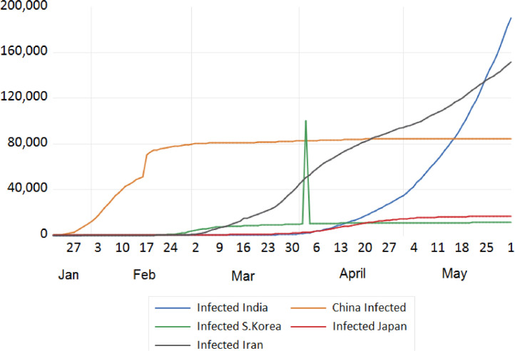
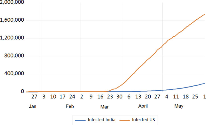
We tried to analyse the infected cases due to COVID-19 between India and European countries, China, Japan, S. Korea, Iran, USA, and Russia. The trend analysis of these comparisons is depicted in Figs. 7, 8 , 9 , and 10 . It has been observed that rate of infection of COVID-19 in India is comparatively lower than that of European countries, USA and Russia (Figs. 7, 9, and 10). This lower rate of infection is due to the strict implementation of lockdown in four different phases in India.

Fig. 8.

Trend analysis of cumulative infected cases of India, China, Japan, South Korea and Iran.

Fig. 9.

Trend analysis of cumulative infected cases of India and USA.

By the time India reported continuous increase in infected cases, European countries had already passed this continuous increasing pandemic phase and measures implemented by them were a lesson for the entire world. In addition to the lockdown, the classification of various zones, containment strategy and various other measures by the Indian Government can be attributed to the comparatively lower infected cases during the period of study.

5.5. Trend analysis of case fatality rates–comparison between India and other nations

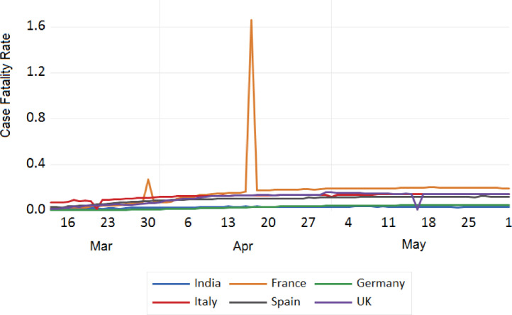
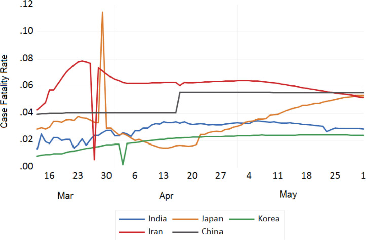
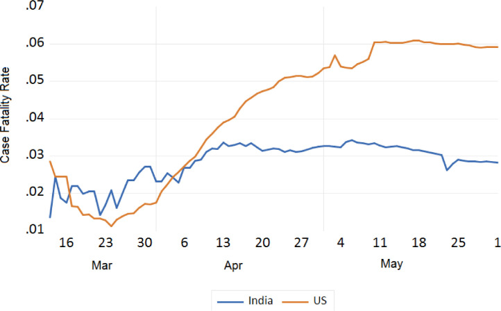
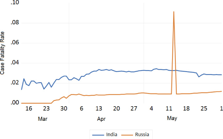
We also tried to analyse the fatality due to COVID-19 between India and European countries, China, Japan, S. Korea, Iran, USA, and Russia. The trend analysis of these comparisons is depicted in Figs. 11 , 12 , 13 , and 14 . It has been observed that the fatality rate due to COVID-19 infection in India is comparatively lower than that of European countries (Fig. 11), USA (Fig. 13), China, Japan and Iran (Fig. 12). This lower fatality rate due to COVID-19 infection is due to the strict implementation of lockdown in four different phases in India.

Fig. 11.

Trend analysis of case fatality rate of India and European Countries.

Fig. 12.

Trend analysis of case fatality rate of India, China, Japan, South Korea and Iran.

Fig. 13.

Trend analysis of case fatality rate of India and USA.

Fig. 14.

Trend analysis of case fatality rate of India and Russia.

6. Conclusion

Compartmental epidemic model: susceptible-exposed-home quarantine-infected-hospital quarantine-recovered is developed to understand the transmitting behaviour of pandemic COVID-19 in human population, very specifically in Bhilwara, a desert town of Rajasthan state in India, where effective control measure TTT(tracking, testing, treatment) was performed to minimise the spread of the disease. Local and global asymptotic stability is established for the endemic equilibrium of the proposed mathematical model. Extensive numerical simulations with real parametric values are performed to establish the analytical results. Statistical Analysis has been performed to analyse the impact of lockdown in different part of the world badly infected by COVID-19 with India. Non-parametric significance test (Mann Whitney test) was performed at 95% and 99% confidence interval of infected cases during the lockdown phases between India and other nations of the world. It is observed that the countries were various measures was implemented had led to good control over the number of infected cases, an increase in the number of recovered cases and improved the fatality rate as a whole. Kruskal - Wallis test is performed to test the null hypothesis for infected cases during the four lockdown phases in India. It is observed that there is a significant difference at both 95% and 99% confidence interval in the infected cases, recovered cases and the case fatality rate during all the four phases of the lockdown with a p value less than 5%. Mann Whitney test was performed to find which two specific phases are responsible for the significant difference and it is observed that there is significant difference in the number of infected cases, number of recovered cases and the case fatality rate between phase 1 and phase 2, phase 2 and phase 3 & phase 3 and phase 4. Time series forecasting model is performed for the infected cases of India and also time series forecasting of actual cases versus predicted cases in India is performed. Also time series forecasting model for the case fatality rate in India and time series forecasting of actual cases versus predicted cases in India is performed.

Author statement

Bimal Kumar Mishra developed the mathematical model with hypothesis and Introduction part.

Ajit Kumar Keshri proved the local stability and simulation was performed by him.

Dinesh Kumar Saini collected the data very specifically of Bhilwara, discussed the different lock down phases.

Syeda Ayesha carried out the statistical analysis.

Binay Kumar Mishra carried out the different suggestions made by the reviewers.

Y S Rao proved the global stability.

Declaration of Competing Interest

The authors declare that they have no known competing financial interests or personal relationships that could have appeared to influence the work reported in this paper.

Appendix 1

We try to establish

$$a_1>0,a_2>0,a_3>0\text{and}{a}_1·a_2>a_3$$ (3′)

To establish the relation (3), we refer Example 1 and Table 2 of Section 4 and after substituting the parametric values we have,

$$\begin{array}{c}{a}_1=\left[0.3+0.05+\left(3*0.01\right)+0.3+0.02+0.07+0.1+0.018\right];\hfill \\ a_1=0.888;\hfill \end{array}$$

$$\begin{array}{c}{a}_2=\left[\left(0.3+0.05+0.01\right)\left(0.3+0.02+0.01\right)\right]\hfill \\ +\left[\left(0.3+0.05+0.01\right)\left(0.07+0.1+0.01+0.018\right)\right]\hfill \\ +\left[\left(0.07+0.1+0.01+0.018\right)\left(0.3+0.02+0.01\right)\right];\hfill \\ a_2=0.25542;\hfill \end{array}$$

$$\begin{array}{c}\hfill a_3=[\left(0.3+0.05+0.01\right)\left(0.3+0.02+0.01\right)\\ \hfill \times \left(0.07+0.1+0.01+0.018\right)]-\left(0.1*0.3*0.3\right);\\ \hfill a_3=0.0145224.\end{array}$$

And $a_1*a_2=0.888*0.25542=0.22681296>a_3$(=0.0145224)

Thus the relation (3) holds.

Appendix 2

We try to establish the relation

$$A_1>0,A_3>0,A_4>0\text{and}\begin{array}{c}{A}_1{A}_2{A}_3>A_3^2+A_1^2{A}_4\\ \Rightarrow A_1{A}_2{A}_3-(A_3^2+A_1^2{A}_4)>0\end{array}$$ (4′)

For this, we refer Example 2 and Table 3 (at equilibrium point $I^{*}=0.057$and $S^{*}=0.6149$) and Table 4 of Section 4. After substituting the parametric values in (4), we have,

$$\begin{array}{c}{A}_1=[\left(0.4*0.0570\right)+0.3+0.05+0.3+0.02+0.07+0.1\hfill \\ +\left(4*0.02\right)+0.03];\hfill \\ \Rightarrow A_1=0.9728.\hfill \end{array}$$

$$\begin{array}{ccc}& & \begin{array}{c}{A}_2=\left[\{\left(0.4*0.057\right)+0.02\}\left(0.3+0.05+0.02\right)\right]\hfill \\ +\left[\{\left(0.4*0.057\right)+0.02\}\left(0.07+0.1+0.02+0.03\right)\right]\hfill \\ +\left[\left(0.3+0.02+0.02\right)\{\left(0.4*0.057\right)+0.02\}\right]\hfill \\ \\ +\left[\left(0.3+0.05+0.02\right)\left(0.07+0.1+0.02+0.03\right)\right]\hfill \\ +\left[\left(0.3+0.05+0.02\right)\left(0.3+0.02+0.02\right)\right]\hfill \\ +\left[\left(0.3+0.02+0.02\right)\left(0.07+0.1+0.02+0.03\right)\right];\hfill \\ \Rightarrow A_2=0.321804.\hfill \end{array}\hfill \\ & & \begin{array}{c}{A}_3=[\left\{\left(0.4*0.057\right)+0.02\right\}\hfill \\ \left(0.3+0.05+0.02\right)\left(0.07+0.1+0.02+0.03\right)]\hfill \\ +\left[\{\left(0.4*0.057\right)+0.02\}\left(0.3+0.05+0.02\right)\left(0.3+0.02+0.02\right)\right]\hfill \\ +[\{\left(0.4*0.057\right)+0.02\}\hfill \\ \left(0.3+0.02+0.02\right)\left(0.07+0.1+0.02+0.03\right)]\hfill \\ +[\left(0.3+0.02+0.02\right)\left(0.07+0.1+0.02+0.03\right)\hfill \\ \left(0.3+0.05+0.02\right)]\hfill \\ -\left(0.4*0.057*0.3*0.02\right)-\left(0.4*0.6149*0.3*0.3\right);\hfill \\ \Rightarrow A_3=0.0174724.\hfill \end{array}\hfill \end{array}$$

$$\begin{array}{c}{A}_4=[\left\{\left(0.4*0.057\right)+0.02\right\}\left(0.3+0.05+0.02\right)\hfill \\ \left(0.07+0.1+0.02+0.03\right)\left(0.3+0.02+0.02\right)]\hfill \\ -\left[\left\{\left(0.4*0.057\right)+0.02\right\}*0.4*0.6149*0.3*0.3\right]\hfill \\ +\left[{\left(0.4\right)}^2*0.6149*0.057*0.3*0.3\right]\hfill \\ -\left[0.4*0.057*0.02*0.3*\left(0.07+0.1+0.02+0.03\right)\right];\hfill \\ \Rightarrow A_4=0.0007117088.\hfill \end{array}$$

$$\begin{array}{c}{A}_1{A}_2{A}_3>A_3^2+A_1^2{A}_4\hfill \\ \Rightarrow A_1{A}_2{A}_3-(A_3^2+A_1^2{A}_4)>0\hfill \\ \Rightarrow 0.9728*0.321804*0.0174724\hfill \\ -\left[{\left(0.0174724\right)}^2+\left\{{\left(0.9728\right)}^2*0.0007117088\right\}\right]>0\hfill \\ \Rightarrow 0.0044909479>0.\hfill \end{array}$$

Thus the relation (4) holds.

References

- 1.https://www.who.int/emergencies/diseases/novel-coronavirus-2019
- 2.Boccaletti S., Ditto W., Mindlin G., Atangana A. Modeling and forecasting of epidemic spreading: the case of Covid-19 and beyond. Chaos, Solitons, Fractals. 2020;135 doi: 10.1016/j.chaos.2020.109794. [DOI] [PMC free article] [PubMed] [Google Scholar]
- 3.Mishra B.K., Keshri A.K., Rao Y.S., Mishra B.K., Mahato B., Ayesha S. COVID-19 created chaos across the globe: three novel quarantine epidemic models. Chaos, Solitons Fractals. 2020;138 doi: 10.1016/j.chaos.2020.109928. [DOI] [PMC free article] [PubMed] [Google Scholar]
- 4.Goh G.K.-M., Uversky V.N., Dunker A.K. Understanding viral transmission behavior via protein intrinsic disorder prediction: corona viruses. J Pathogens. 2012;2012:13. doi: 10.1155/2012/738590. (2020), Article ID 738590. [DOI] [PMC free article] [PubMed] [Google Scholar]
- 5.WHO; Geneva: 2020. Modes of transmission of virus causing COVID-19: implications for IPC precaution recommendations. https://www.who.int/news-room/commentaries/detail/modes-of-transmission-of-virus-causing-covid-19-implications-for-ipc-precaution-recommendations. [Google Scholar]
- 6.Soukhovolsky V., Kovalev A., Pitt A., Kessel B. A new modelling of the COVID 19 pandemic. Chaos, Solitons Fractals. 2020;139 doi: 10.1016/j.chaos.2020.110039. [DOI] [PMC free article] [PubMed] [Google Scholar]
- 7.Kassa S.M., Njagarah J.B., Terefe Y.A. Analysis of the mitigation strategies for COVID-19: from mathematical modelling perspective. Chaos, Solitons Fractals. 2020;138 doi: 10.1016/j.chaos.2020.109968. [DOI] [PMC free article] [PubMed] [Google Scholar]
- 8.Hernandez-Vargas E.A., Velasco-Hernandez J.X. In-host mathematical modelling of covid-19 in humans. Ann Rev Control. 2020 doi: 10.1016/j.arcontrol.2020.09.006. [DOI] [PMC free article] [PubMed] [Google Scholar]
- 9.Wang S., Pan Y., Wang Q., Miao H., Brown A.N., Rong L. Modeling the viral dynamics of SARS-CoV-2 infection. Math Biosci. 2020;328 doi: 10.1016/j.mbs.2020.108438. [DOI] [PMC free article] [PubMed] [Google Scholar]
- 10.Vespignani A., Tian H., Dye C., Lloyd-Smith J.O., Eggo R.M., Shrestha M. Modelling covid-19. Nat Rev Phys. 2020;2(6):279–281. doi: 10.1038/s42254-020-0178-4. [DOI] [PMC free article] [PubMed] [Google Scholar]
- 11.Batistela C.M., Correa D.P., Bueno Á.M., Piqueira J.R.C. SIRSi compartmental model for COVID-19 pandemic with immunity loss. Chaos, Solitons Fractals. 2020 doi: 10.1016/j.chaos.2020.110388. [DOI] [PMC free article] [PubMed] [Google Scholar]
- 12.Kudryashov N.A., Chmykhov M.A., Vigdorowitsch M. Analytical features of the SIR model and their applications to COVID-19. Appl Math Modell. 2021;90:466–473. doi: 10.1016/j.apm.2020.08.057. [DOI] [PMC free article] [PubMed] [Google Scholar]
- 13.Valba O.V., Avetisov V.A., Gorsky A.S., Nechaev S.K. Evaluating ideologies of coronacrisis-related self-isolation and frontiers closing by SIR compartmental epidemiological model. Beacon J Stud Ideol Ment Dimens. 2020;3(2) 2020. [Google Scholar]
- 14.Jiang, J., Jiang, L., Li, G., Luo, J., Wang, M., & Xu, H. (2020). Prediction of the epidemic trends of COVID-19 by the improved dynamic SEIR model.
- 15.Devlin, H. (2020, May 15). Regional differences in COVID-19 transmission rate emerge in England. Retrieved from The Guardian, https://www.theguardian.com/world/2020/may/15/regional-differences-in-covid-19-transmission-rate-emerge-in-england
- 16.Zhang J., Litvinova M., Wang W., Wang Y., Deng X., Chen X. Evolving epidemiology and transmission dynamics of coronavirus disease 2019 outside Hubei province, China: a descriptive and modelling study. Lancet Infect Dis. 2020;20(7):793–802. doi: 10.1016/S1473-3099(20)30230-9. [DOI] [PMC free article] [PubMed] [Google Scholar]
- 17.Fanelli Duccio, Piazza Francesco. Analysis and forecast of COVID-19 spreading in China, Italy and France. Chaos Solitons Fractals. 2020;134 doi: 10.1016/j.chaos.2020.109761. [DOI] [PMC free article] [PubMed] [Google Scholar]
- 18.Ndaïrou Faïçal, Area Iván, Nieto Juan J., Torres Delfim F.M. Mathematical modeling of COVID-19 transmission dynamics with a case study of Wuhan. Chaos Solitons Fractals. 2020;135 doi: 10.1016/j.chaos.2020.109846. [DOI] [PMC free article] [PubMed] [Google Scholar]
- 19.Ribeiro Matheus Henrique Dal Molin, Silva Ramon Gomes da, Mariani Viviana Cocco, Coelho Leandro dos Santos. Short-term forecasting COVID-19 cumulative confirmed cases: perspectives for Brazil. Chaos Solitons Fractals. 2020;135 doi: 10.1016/j.chaos.2020.109853. [DOI] [PMC free article] [PubMed] [Google Scholar]
- 20.Tagliazucchi E., Balenzuela P., Travizano M., Mindlin G.B., Mininni P.D. Lessons from being challenged by COVID-19. Chaos Solitons Fractals. 2020;137 doi: 10.1016/j.chaos.2020.109923. [DOI] [PMC free article] [PubMed] [Google Scholar]
- 21.Brauer Fred, Castillo-Chavez Carlos, Feng Zhilan. Springer; New York: 2019. Mathematical models in epidemiology. [Google Scholar]
- 22.Giordano Giulia, Blanchini Franco, Bruno Raffaele, Colaneri Patrizio, Filippo Alessandro Di, Matteo Angela Di. Modelling the COVID-19 epidemic and implementation of population-wide interventions in Italy. Nat Med. 2020;26:855–860. doi: 10.1038/s41591-020-0883-7. [DOI] [PMC free article] [PubMed] [Google Scholar]
- 23.Li Y., Muldowney J.S. On Bendixson′ s Criterion. J Diff Eqns. 1993;106(1):27–39. [Google Scholar]
- 24.Li M.Y., Muldowney J.S. A geometric approach to global-stability problems. SIAM J Math Anal. 1996;27(4):1070–1083. [Google Scholar]
- 25.Berhe Hailay Weldegiorgis, Makinde Oluwole Daniel, Theuri David Mwangi. Modelling the dynamics of direct and pathogens-induced dysentery diarrhoea epidemic with controls. J Biol Dyn. 2019;13(1):192–217. doi: 10.1080/17513758.2019.1588400. [DOI] [PubMed] [Google Scholar]
- 26.Wang L., Li M.Y., Kirschner D. Mathematical analysis of the global dynamics of a model for HTLV-I infection and ATL progression. Math Biosci. 2002;179(2):207–217. doi: 10.1016/s0025-5564(02)00103-7. [DOI] [PubMed] [Google Scholar]