Reinforcement learning-based decision support system for COVID-19

Abstract

Globally, informed decision on the most effective set of restrictions for the containment of COVID-19 has been the subject of intense debates. There is a significant need for a structured dynamic framework to model and evaluate different intervention scenarios and how they perform under different national characteristics and constraints. This work proposes a novel optimal decision support framework capable of incorporating different interventions to minimize the impact of widely spread respiratory infectious pandemics, including the recent COVID-19, by taking into account the pandemic's characteristics, the healthcare system parameters, and the socio-economic aspects of the community. The theoretical framework underpinning this work involves the use of a reinforcement learning-based agent to derive constrained optimal policies for tuning a closed-loop control model of the disease transmission dynamics.

1. Introduction

Mankind has witnessed several pandemics in the past including plague, leprosy, smallpox, tuberculosis, AIDS, cholera, and malaria [1], [2], [3]. The historic timeline of pandemics suggests that the frequency of occurrence is increasing and in an era wherein globalization is happening at an accelerated pace, we are more likely to confront many such threats in the near future [4], [5], [6], [7]. Hence, it is quite imperative to consolidate the lessons learned out of our experience with the current COVID-19 global pandemic towards building a resilient community with people prepared to prevent, respond to, combat, and recover from the social, health, and economic impacts of pandemics. Preparedness is a key factor in mitigating pandemics. It encompasses inculcating awareness about the outbreaks and fostering response strategies to ensure avoiding loss of life and socio-economic havoc. While the emergence of a harmful microorganism with pandemic potential may be unpreventable, pandemics can be prevented [4]. Preparedness includes technological readiness to identify pathogen identity, fostering drug discovery, and developing reliable theoretical models for prediction, analysis, and control of pandemics.

Lately, collaborative efforts among epidemiologists, microbiologists, geneticists, anthropologists, statisticians, and engineers have complimented the research in epidemiology and have paved the way for improved epidemic detection and control [8], [9]. There exists an enormous amount of studies concerning epidemiological models and the use of such theoretic models in deriving cost-effective decisions for the control of epidemics. Sliding mode control, tracking control, optimal control, and adaptive control methods have been applied to control the spread of malaria, influenza, zika virus, etc. [7], [10], [11], [12]. Optimal control methods are used to identify ideal intervention strategies for mitigating epidemics that accounts for the cost involved in implementing pharmaceutical or nonpharmaceutical interventions (PI or NPI). For instance, in [13], a globally-optimal vaccination strategy for a general epidemic model (susceptible-infected-recovered (SIR)) is derived using the Hamilton-Jacobi-Bellman (HJB) equation. It is pointed out that such solutions are not unique and a closer analysis is needed to derive cost-effective and physically realizable strategies. In [14], the hyperchaotic behavior of epidemic spread is analyzed using the SEIR (susceptible-exposed-infected-recovered) model by modeling nonlinear transmissibility.

Even though various optimization algorithms were used to derive time-optimal and resource-optimal solutions for general epidemic models, only a few of the possibilities have been explored for COVID-19 in particular. The majority of the model-based studies for COVID-19 discuss various scenario analyses such as the influence of isolation only, vaccination only, and combining isolation with vaccination on the overall disease transmission [15], [16], [17], [18], [19]. Even though several works focused on evaluating the influence of various control interventions on the mitigation of COVID-19, only very few literature discuss the derivation of an active intervention strategy from a control-theoretic viewpoint. In [20], the authors discuss an SEIR model-based optimal control strategy to deploy strict public-health control measures until the availability of a vaccine for COVID-19. Simulation results show that the derived optimal solution is more effective compared to constant-strict control measures and cyclic control measures. In [21], optimal and active closed-loop intervention policies are derived using quadratic programming method to mitigate COVID-19 in the United States while accounting for death and hospitalizations constraints.

In this paper, we propose the development and use of a reinforcement learning-based closed-loop control strategy as a decision support tool for mitigating COVID-19. Reinforcement Learning (RL) is a category of machine learning that has proved promising in handling control problems that demand multi-stage decision support [22]. With the exponential advancement in computing methods, machine learning-based methods are becoming increasingly useful in many biomedical applications. For instance, RL-based controllers have been used to make intelligent decisions in the area of drug dosing for patients undergoing hemodialysis, sedation, and treatment for cancer or schizophrenia [22], [23], [24], [25], [26], [27]. Similarly, machine-learning experts are contributing to the area of epidemics detection and control [9], [28], [29]. In [6], the RL-based method is used to make optimal decisions regarding the announcement of an anthrax outbreak. Data on the benefits of true alarms and the cost associated with false alarms are used to formulate and solve the problem of the anthrax outbreak announcement in a RL-framework. Decisions concerning the declaration of an outbreak are evaluated by defining six states such as no outbreak, waiting day 1, waiting day 2, waiting day 3, waiting day 4, and outbreak detected.

Using RL-based closed-loop control, at each stage, decisions can be revised according to the response of the system that embodies a multitude of uncertainties. In the case of a mathematical model that represents COVID-19 disease transmission dynamics, uncertainties include system disturbance such as a sudden increase in exposure rate due to school reopening or reduced transmission due to increased compliance of people or any other unmodeled system dynamics. The underlying strategy behind RL-based methods is the concept of learning an ideal policy from the agent's experience with the environment. Basically, the agent (actor) interacts with the system (environment) by applying a set of feasible control inputs and learns a favorable control policy based on the values attributed to each intervention-response pair.

The mathematical formulation of the optimal control problem under RL-framework allows it to be used as a tool for optimizing intervention policies. The focus of this paper is to present such a learning-based model-free closed-loop optimal and effective decision support tool for limiting the spread of COVID-19. We use a mathematical model that captures COVID-19 transmission dynamics in a population as a simulation model instead of the real system to collect interaction data (intervention-response) required for training the RL-based controller. The main contributions of this work can be summarized as follows: (1) Novel disease spread model that accounts for the influence of NPIs on the overall disease transmission rate and specific infection rates during the asymptomatic and symptomatic periods, (2) Development of an RL-based closed-loop controller for mitigating COVID-19, and (3) Design of reward function to account for cost and hospital saturation constraints.

The organization of this paper is as follows. In Section 2, a mathematical model for COVID-19 and the development of a RL-based controller are presented. Simulation results for two case studies are given in Section 3. Robustness of the controller with respect to various disturbances are also discussed in this section. Conclusions and scope for future research are presented in Section 4.

2. Methods

2.1. RL-framework

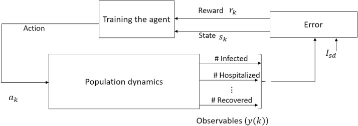
The proposed approach incorporates the development of a decision support system that utilizes a $Q$-learning-based approach to derive optimal solutions with respect to certain predefined cost objectives. The main components of the RL-framework include an environment (system or process) whose output signals need to be regulated and an RL-agent that explores the RL environment to gain knowledge about the system dynamics towards deriving an appropriate control strategy. Schematic of such a learning framework is shown in Fig. 1 , where the population dynamics pertaining to COVID-19 represents the RL environment, and control interventions represent the actions imposed by the RL-agent.

Fig. 1.

Schematic representation of reinforcement learning framework for COVID-19. This learning-based controller design is predicated on the observed data obtained as a response to an action imposed on the population. The response data $y(k)$ include the number of infected, hospitalized, recovered, etc. Error is the difference between observed number of severely infected and desired number of severely infected ($I_{\mathit{sd}}$). Learning is facilitated based on the reward $r_k$ incurred according to the state ($s_k$), action($a_k$), new state ($s_{k+1}$).

In this paper, Watkin's $Q$-learning algorithm which does not demand an accurate or complete system model is used to train the RL-agent [27], [30]. The control objective is to derive an optimal control input that minimizes the infected population while minimizing the cost associated with interventions. The RL-based methodology provides a framework for an agent to interact with its environment and receive rewards based on observed states and actions taken. In $Q$-table, the desirability of an action when in a particular system state is encoded in terms of a quantitative value calculated with respect to the reward incurred for an intervention-response pair. The goal of an RL-based agent is to learn the best sequence of actions that can maximize the expected sum of returns (rewards). Note that the RL-based controller design is model-free and does not rely on parameter knowledge of the system but it utilizes the intervention-response observations from the environment. Specifically, the RL-based controller design discussed in this paper requires the information on the number of susceptibles and severely infected cases. As mentioned earlier, instead of the real system we use a simulation model to obtain intervention-response data to train the RL-agent. The model is given by [20]:

$$\frac{\mathrm{d}S(t)}{\mathrm{d}t}=-\beta (t)S(t)-{\mu }^{\prime }S(t),S(0)=S_0,$$ (1)

$$\frac{\mathrm{d}{E}_{\mathrm{m}}(t)}{\mathrm{d}t}=p\beta (t)S(t)-{\tau }_{\mathrm{L}}{E}_{\mathrm{m}}(t)-{\mu }^{\prime }{E}_{\mathrm{m}}(t)+p\rho ,E_{\mathrm{m}}(0)=E_{\mathrm{m}0},$$ (2)

$$\frac{\mathrm{d}{I}_{\mathrm{am}}(t)}{\mathrm{d}t}={\tau }_{\mathrm{L}}{E}_{\mathrm{m}}(t)-{\tau }_{\mathrm{I}}{I}_{\mathrm{am}}(t)-{\mu }^{\prime }{I}_{\mathrm{am}}(t),I_{\mathrm{am}}(0)=I_{\mathrm{am}0},$$ (3)

$$\frac{\mathrm{d}{I}_{\mathrm{m}}(t)}{\mathrm{d}t}={\tau }_{\mathrm{I}}{I}_{\mathrm{am}}(t)-({\lambda }_1+{\mu }^{\prime })I_{\mathrm{m}}(t),I_{\mathrm{m}}(0)=I_{\mathrm{m}0},$$ (4)

$$\frac{\mathrm{d}{R}_{\mathrm{m}}(t)}{\mathrm{d}t}={\lambda }_1{I}_{\mathrm{m}}(t)-{\mu }^{\prime }{R}_{\mathrm{m}}(t),R_{\mathrm{m}}(0)=R_{\mathrm{m}0},$$ (5)

$$\frac{\mathrm{d}{E}_{\mathrm{s}}(t)}{\mathrm{d}t}=(1-p)\beta (t)S(t)-{\tau }_{\mathrm{L}}{E}_{\mathrm{s}}(t)-{\mu }^{\prime }{E}_{\mathrm{s}}(t)+(1-p)\rho ,E_{\mathrm{s}}(0)=E_{\mathrm{s}0},$$ (6)

$$\frac{\mathrm{d}{I}_{\mathrm{as}}(t)}{\mathrm{d}t}={\tau }_{\mathrm{L}}{E}_{\mathrm{s}}(t)-{\tau }_{\mathrm{I}}{I}_{\mathrm{as}}(t)-{\mu }^{\prime }{I}_{\mathrm{as}}(t),I_{\mathrm{as}}(0)=I_{\mathrm{as}0},$$ (7)

$$\frac{\mathrm{d}{I}_{\mathrm{s}}(t)}{\mathrm{d}t}={\tau }_{\mathrm{I}}{I}_{\mathrm{as}}(t)-({\lambda }_2+{\mu }^{\prime }+\mu )I_{\mathrm{s}}(t),I_{\mathrm{s}}(0)=I_{\mathrm{s}0},$$ (8)

$$\frac{\mathrm{d}{R}_{\mathrm{s}}(t)}{\mathrm{d}t}={\lambda }_2{I}_{\mathrm{s}}(t)-{\mu }^{\prime }{R}_{\mathrm{s}}(t),R_{\mathrm{s}}(0)=R_{\mathrm{s}0},$$ (9)

$$\frac{\mathrm{d}D(t)}{\mathrm{d}t}=\mu I_{\mathrm{s}}(t)+{\mu }^{\prime }N(t),D(0)=D_0,$$ (10)

with

$$N(t)=S(t)+E(t)+A(t)+I(t)+R(t),N(0)=N_0,$$ (11)

$$E(t)=E_{\mathrm{m}}(t)+E_{\mathrm{s}}(t),E(0)=E_0,$$ (12)

$$I_{\mathrm{a}}(t)=I_{\mathrm{am}}(t)+I_{\mathrm{as}}(t),I_{\mathrm{a}}(0)=I_{\mathrm{a}0},$$ (13)

$$I(t)=I_{\mathrm{m}}(t)+I_{\mathrm{s}}(t),I(0)=I_0,$$ (14)

$$R(t)=R_{\mathrm{m}}(t)+R_{\mathrm{s}}(t),R(0)=R_0,$$ (15)

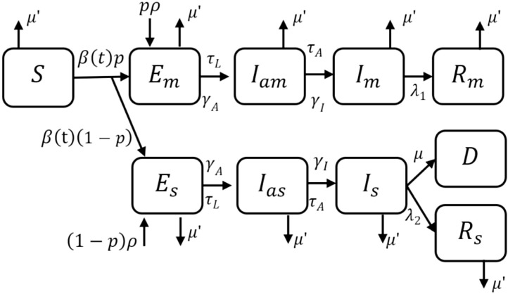
where $S(t)$ denotes the number of susceptibles, $E_{\mathrm{m}}(t)$ and $I_{\mathrm{m}}(t)$ denote the number of exposed and mildly infected symptomatic patients, respectively, $R_{\mathrm{m}}(t)$ is the number of recovered patients from mild infection, $E_{\mathrm{s}}(t)$ and $I_{\mathrm{s}}(t)$ denote the number of exposed and severely infected symptomatic patients, $I_{\mathrm{am}}(t)$ and $I_{\mathrm{as}}(t)$ denote asymptomatic patients who later on move to mildly and severely infected compartments, respectively, and $D(t)$ is the total number of direct and indirect death due to COVID-19 [20]. Out of the total number of exposed, a larger proportion ($E_{\mathrm{m}}(t)>80\%\mathrm{of}E(t)$) develop mild infection and rest ($E_{\mathrm{s}}(t)$) develop severe infection after a delay. The intervention-response data required for training the RL-agent is derived using the mathematical model (1), (2), (3), (4), (5), (6), (7), (8), (9), (10). Fig. 2 shows the corresponding compartmental representation, where the state vector $x(t)={[S(t),E_{\mathrm{m}}(t),I_{\mathrm{am}}(t)\text{,}{I}_{\mathrm{m}}(t),R_{\mathrm{m}}(t),E_{\mathrm{s}}(t),I_{\mathrm{as}}(t),I_{\mathrm{s}}(t),R_{\mathrm{s}}(t),D(t)]}^{\mathrm{T}}$ (Table 1 ).

Fig. 2.

Compartmental model (1), (2), (3), (4), (5), (6), (7), (8), (9), (10) of COVID-19 that accounts for differential disease severity and import of exposed cases into the population [20].

Table 1.

Parameter descriptions for model (1), (2), (3), (4), (5), (6), (7), (8), (9), (10), (11), (12), (13), (14), (15), (16), (17), (18), (19), (20), (21).

Parameter	Parameter description
$S(t)$	Susceptibles
$E_{\mathrm{m}}(t)$, $E_{\mathrm{s}}(t)$	Exposed individuals with mild or severe infection
$I_{\mathrm{am}}(t)$, $I_{\mathrm{as}}(t)$	Infectious asymptomatic patients with mild or severe infection
$I_{\mathrm{m}}(t)$, $I_{\mathrm{s}}(t)$	Infectious symptomatic patients with mild or severe infection
$R_{\mathrm{m}}(t)$, $R_{\mathrm{s}}(t)$	Recovered patients who had mild or severe infection
$\beta (t)$	Exposure rate
${\tau }_{\mathrm{L}}$	Waiting rate to viral shedding
${\tau }_{\mathrm{I}}$	Waiting rate to symptom onset
${\lambda }_1$	Recovery rate of mildly infected patients
${\lambda }_2$	Recovery rate of severely infected patients
$p$	Fraction of mild infections
$m$	Modification factor to account for reduced transmission factor of severely infected
${\theta }_{\mathrm{c}}$	Case-fatality related to severe infection
${\mu }_{\mathrm{H}}$	Natural death related to hospital saturation
$H$	Hospital capacity
${\mu }^{\prime }$	Rate of indirect death due to COVID-19
$\mu$	Rate of direct death due to COVID-19
$\rho$	Immigration or import rate
${\gamma }_{\mathrm{A}}$	Infection rate related to $I_{\mathrm{am}}$ and $I_{\mathrm{as}}$ (Asymptomatic transmission)
${\gamma }_{\mathrm{I}}$	Infection rate related to $I_{\mathrm{m}}$ and $I_{\mathrm{s}}$ (Symptomatic transmission)

The transmission parameter $\beta (t)$ in (1)–(10) is given by

$$\beta (t)=(1-u_1(t))\left({\gamma }_{\mathrm{A}}(1-u_2(t))(I_{\mathrm{am}}(t)+I_{\mathrm{as}}(t))+{\gamma }_{\mathrm{I}}(1-u_3(t))(I_{\mathrm{m}}(t)+{\mathrm{mI}}_{\mathrm{s}}(t))\right),$$ (16)

where

$${\gamma }_{\mathrm{A}}={\gamma }_{\mathrm{I}}=\frac{R_0}{S_0}{\lambda }_1{\tau }_{\mathrm{I}}\frac{{\mu }_{\min }+{\lambda }_2}{({\lambda }_1+p{\tau }_{\mathrm{I}})({\mu }_{\min }+{\lambda }_2)+m{\lambda }_1{\tau }_{\mathrm{I}}(1-p)},$$ (17)

$${\mu }^{\prime }=\left\{\begin{array}{cc}0\hfill & \mathrm{if}{I}_{\mathrm{s}}(t)<H\hfill \\ {\mu }_{\mathrm{H}}\hfill & \mathrm{if}{I}_{\mathrm{s}}(t)\ge H\hfill \end{array}\right),$$ (18)

$$\mu =\left\{\begin{array}{cc}{\mu }_{\min }\hfill & \mathrm{if}{I}_{\mathrm{s}}(t)<H\hfill \\ {\mu }_{\max }\hfill & \mathrm{if}{I}_{\mathrm{s}}(t)\ge H\hfill \end{array}\right),$$ (19)

$${\mu }_{\min }={\lambda }_2\frac{{\theta }_{\mathrm{c}}}{1-{\theta }_{\mathrm{c}}},$$ (20)

$${\mu }_{\max }=2{\mu }_{\min }.$$ (21)

Table 1 details the parameter descriptions pertaining to model (1), (2), (3), (4), (5), (6), (7), (8), (9), (10).

The obvious increase in the disease exposure of the population in susceptible compartment following the increase in the number of $I_{\mathrm{am}}(t)$, $I_{\mathrm{as}}(t)$, $I_{\mathrm{m}}(t)$, and $I_{\mathrm{s}}(t)$ is modeled in (16), where ${\gamma }_{\mathrm{A}}$ and ${\gamma }_{\mathrm{I}}$ are the rates at which the population with asymptomatic and symptomatic disease manifestation infect the susceptible population, respectively, $u_i(t)$, $i=1,2,3$, account for the influence of various control interventions on the transmission rate of the virus, and $m$ is the modification parameter used to model the reduced transmission rate of the severely sick population as they will be moved to hospital hence under strict isolation. Specifically, $u_1(t)$ accounts for the impact of travel restrictions on the overall mobility and interactions of the population in various infected compartments, $u_2(t)$ accounts for the efforts to reduce the infection rate ${\gamma }_{\mathrm{A}}$ (during the asymptomatic period). Asymptomatic patients often remain undetected and hence awareness campaigns to increase the compliance of people can reduce the chance of infection spread during the asymptomatic period. Specific efforts to reduce the infection rate ${\gamma }_{\mathrm{I}}$ (during symptomatic period) is accounted by $u_3(t)$. This includes hospitalization of severely infected ($I_{\mathrm{s}}(t)$) and isolation/quarantine of mildly infected ($I_{\mathrm{m}}(t)$) that will reduce the chance of infection spread during the symptomatic period. The viability of each of the control inputs $u_i(t)$, $i=1,2,3$, in controlling the overall transmission rate $\beta (t)$ is different, an increase in $u_1(t)$ results in an overall reduction in $\beta (t)$ (e.g. lockdown or travel ban influence interaction rate among $I_{\mathrm{am}}(t)$, $I_{\mathrm{as}}(t)$, $I_{\mathrm{m}}(t)$, and $I_{\mathrm{s}}(t)$), where as an increase in $u_2(t)$ (e.g. increased hygiene habits due awareness) or $u_3(t)$ (e.g. strict exposure control measures and bio hazard handling protocols at healthcare facilities) reduces the disease transmission through $I_{\mathrm{a}}(t)$ or $I(t)$, respectively.

It should be noted that apart from death due to COVID-19, there can be indirect fatalities due to the overwhelming of hospitals and the allocation of hospital resources for the management of the pandemic. The indirect fatalities account for the death of the patients due to the unavailability of medical attention or inaccessibility of hospitals. In (18), the death rate indirectly related to COVID-19 is denoted as $({\mu }^{\prime })$, and it is set to zero if the active number of the severely infected population is below the hospital capacity ($H$) and is set to ${\mu }_{\mathrm{H}}$ whenever hospitals are saturated, where ${\mu }_{\mathrm{H}}$ models the increase in the mortality rate due to inaccessibility to hospitals. Similarly, direct death due to COVID-19 ($\mu$) can also increase significantly when hospitals saturate, hence ${\mu }_{\max }$ is set to double when $I_{\mathrm{s}}(t)\ge H$ [20].

In the control theory view point, the model (1), (2), (3), (4), (5), (6), (7), (8), (9), (10), (11), (12), (13), (14), (15), (16), (17), (18), (19), (20), (21) can be written in the form

$$\begin{array}{cc}\hfill \frac{\mathrm{d}x(t)}{\mathrm{d}t}& =f(x(t),u(t)),\hfill \\ \hfill y(t)& =h(x(t)),\hfill \end{array}$$ (22)

where $x(t)\in {\mathcal{R}}^{10}$ is the state vector that model the dynamics in the compartments shown in Fig. 2, $u(t)\in {\mathcal{R}}^3$ is the control input, and $y(t)\in {\mathcal{R}}^2$ is the output (observations) of the system, $y(t)={[y_1(t),y_2(t)]}^{\mathrm{T}}$, where $y_1(t)=x_1(t)$ and $y_2(t)=x_8(t)$. Similarly, in the finite Markov decision process (MDP) framework, the system (environment) dynamics are modeled in terms of finite sequences $\mathcal{S}$, $\mathcal{A}$, $\mathcal{R}$, and $\mathcal{P}$, where $\mathcal{S}$ is a finite set of states, $\mathcal{A}$ a finite set of actions defined for the states $s_k\in \mathcal{S}$, $\mathcal{R}$ represents the reward function that guides the agent in accordance to the desirability of an action $a_k\in \mathcal{A}$, and $\mathcal{P}$ is a state transition probability matrix. The state transition probability matrix ${\mathcal{P}}_{a_k}(s_k,s_{k+1})$ gives the probability that an action $a_k\in \mathcal{A}$ takes the state $s_k\in \mathcal{S}$ to the state $s_{k+1}$ in a finite time step. Furthermore, the discrete states in the finite sequence $\mathcal{S}$ are represented as ${({\mathcal{S}}_i)}_{i\in I^{+}}$, where $I^{+}\triangleq \{1,2,\dots ,q\}$ and $q$ denotes the total number of states. Likewise, the discrete actions in the finite sequence $\mathcal{A}$ are represented as ${({\mathcal{A}}_j)}_{j\in J^{+}}$, where $J^{+}\triangleq \{1,2,\dots ,q^{\prime }\}$ and $q^{\prime }$ denotes the total number of actions. The transition probability matrix $\mathcal{P}$ can be formulated based on the system dynamics (22). Note that, since the $Q$-learning framework does not require $\mathcal{P}$ for deriving the optimal control policy, we assume $\mathcal{P}$ is unknown [24], [27].

In the case of epidemic control, the goal is to derive an optimal control sequence to take the system from a nonzero initial state to a desired low infectious state. This problem of deriving action sequence for bringing down the number of infected people requires multi-stage decision making based on the response of the population to various kinds of control interventions. Note that, changes in the overall population dynamics in response to interventions depend upon how far people comply with the restrictions imposed by the government. As shown in Fig. 1, this can be achieved by using the RL algorithm defined/built on the MDP framework by iteratively evaluating action-response sequences observed from system [31], [32].

2.2. Training the agent

RL-based learning phase starts with an initial arbitrary policy, for instance with a $Q$-table with zero entries. $Q$-table is a mapping from states $s_k\in \mathcal{S}$ to a predefined set of interventions $a_k\in \mathcal{A}$ [32]. Each entry of the $Q$-table ($Q_k(s_k,a_k)$) associates an action in the finite sequence ${({\mathcal{A}}_j)}_{j\in J^{+}}$ to a state of the finite sequence ${({\mathcal{S}}_i)}_{i\in I^{+}}$. In the case of epidemic control, a policy represents a series of interventions that have to be imposed on the population to shift the initial status of the environment to a targeted status which is equivalent to the desired set of system states. With respect to a learned $Q$-table, a policy is a sequence of decisions embedded as values in $Q$-table which corresponds to decisions such as “if in state $s_k$, take the ideal action $a_k\in \mathcal{A}$”.

As shown in Fig. 1, during the training phase, the agent imposes control actions ($a_k$) on the RL environment and as the agent gains more and more experience (observations) from the environment the initial arbitrary intervention policy is iteratively updated towards an optimal intervention policy. One of the key factors that helps the agent to assess the desirability of an action and guides it towards the optimal intervention policy is the reward function. Reward function associates an action $a_k$ with a numerical value $r_{k+1}\in ℝ$ (reward) with respect to the state transition $s_k\to s_{k+1}$ of the environment in response to that action. Reward incurred depends on the ability of the last action in transitioning the system states towards the target state or goal state ($G_{\mathrm{s}}$). The reward can be negative or positive for inappropriate or appropriate actions, respectively.

An optimal intervention policy is derived by maximizing the expected value ($E[·]$) of the discounted reward ($r_k$) that the agent receives over an infinite horizon denoted as

$$J(r_k)=E\left[\sum _{k=1}^{\infty }{\theta }^{(k-1)}{r}_k\right],$$ (23)

where the discount rate parameter $\theta \in [0,1]$ represents the importance of immediate and future rewards. With a value of $\theta =0$, the agent considers only the immediate reward, whereas for $\theta$ approaching 1 it considers immediate and future rewards. Based on the experience gained by the agent at each time step $k=1,2,\dots$, the $Q$-table is updated iteratively as

$$Q_k(s_k,a_k)⟵Q_{k-1}(s_k,a_k)+{\eta }_k(s_k,a_k)[r_{k+1}+\theta {max}_{a_{k+1}}{Q}_{k-1}(s_{k+1},a_{k+1})-Q_{k-1}(s_k,a_k)],$$ (24)

where ${\eta }_k(s_k,a_k)\in [0,1)$ is the learning rate. A tolerance parameter $\delta$, $\mathrm{\Delta }{Q}_k\triangleq |Q_k-Q_{k-1}|\le \delta$ is used to specify minimum threshold of convergence [30], [32], [33].

2.3. Reward

As shown in Fig. 1, learning is facilitated based on the reward ($r_k$) incurred according to the state ($s_k$), action ($a_k$), and new state ($s_{k+1}$). The control interventions (actions) imposed on the population basically reduce the disease transmission rate as depicted in (16). As the vaccine for COVID-19 is not approved yet, the control measures against this disease broadly rely on two major factors, namely, I) non-pharmaceutical interventions (NPIs) such as restriction on the social gathering, closure of institutes, and isolation; and II) available pharmaceutical interventions (PIs) such as hospital care with supporting medicines and equipment such as ventilators. Constraints in the health care system such as the number of medical personnel, intensive care beds, COVID-19 testing capacity, COVID-19 isolation and quarantine capacity, dedicated hospitals, and ventilators, as well as the compliance of the society with the interventions are the major challenges for health care system.

The choice of the reward function is critical in guiding the RL-agent towards an optimal intervention policy that will drive the population dynamics to a desired low infectious state while minimizing the socio-economic cost involved. Hence, the reward $r_{k+1}$ is designed to incorporate the influence of three factors

• (1)$r_{k+1}^1$ is used to penalize the agent if $I_{\mathrm{s}}(t)$ exceeds hospital saturation capacity $H$.
• (2)$r_{k+1}^2$ is used to assign a proportional reward to the RL-agent's actions that reduce $I_{\mathrm{s}}(t)$.
• (3)$r_{k+1}^3$ is used to reward/penalize the agent according to the cost associated with the implementation of various control interventions.

The reward $r_{k+1}$ in (24) is calculated as:

$$r_{k+1}^1=\left\{\begin{array}{cc}-1\hfill & \mathrm{if}{I}_{\mathrm{s}}((k+1)T)>H,\hfill \\ 0\hfill & \mathrm{otherwise},\hfill \end{array}\right)$$ (25)

$$r_{k+1}^2=\left\{\begin{array}{cc}\frac{e((k+1)T)-e(\mathrm{kT})}{e(\mathrm{kT})}\hfill & \mathrm{if}e((k+1)T)<e(\mathrm{kT}),\hfill \\ 0\hfill & \mathrm{if}e((k+1)T)\ge e(\mathrm{kT}),\hfill \end{array}\right)$$ (26)

$$r_{k+1}^3=\left\{\begin{array}{cc}+1.3\hfill & \mathrm{if}{c}_{a_k}=\text{very low cost},\hfill \\ +1.2\hfill & \mathrm{if}{c}_{a_k}=\text{low cost},\hfill \\ +1\hfill & \mathrm{if}{c}_{a_k}=\text{medium cost},\hfill \\ -1\hfill & \mathrm{if}{c}_{a_k}=\text{high cost},\hfill \end{array}\right)$$ (27)

where $e(\mathrm{kT})=I_{\mathrm{s}}(\mathrm{kT})-I_{\mathrm{sd}}$, $I_{\mathrm{sd}}$ is the desired value of $I_{\mathrm{s}}(t)$, $\mathrm{kT}\le t<(k+1)T$, and $c_{a_k}$ is the cost associated with each action set. In (27), very low cost, low cost, medium cost, and high cost action represent a predefined combination of actions that are associated with a range of cost such as 0–30%, 20–50%, 30–70%, and 30–90%, respectively (see Table 3). The total reward is:

$$r_{k+1}=r_{k+1}^1+r_{k+1}^2+{\beta }_{\mathrm{w}}{r}_{k+1}^3,$$ (28)

where ${\beta }_{\mathrm{w}}$ is used to relatively weigh the cost of interventions over the infection spread.

Table 3.

Action set, $a_k\in \mathcal{A}$$,{({\mathcal{A}}_j)}_{j\in J^{+}}$, $J^{+}\triangleq \{1,2,\dots ,q^{\prime }\}$, $q^{\prime }=20$.

$j\to$	1	2	3	4	5	6	7	8	9	10	11	12	13	14	15	16	17	18	19	20
$u_1$	0	0	0	0.2	0.2	0.5	0.5	0.5	0.5	0	0.7	0.7	0.7	0.7	0.7	0.9	0.9	0.9	0.9	0.9
$u_2$	0	0	0.3	0	0	0	0	0.3	0.3	0.3	0	0.3	0.5	0.3	0.5	0	0.3	0.5	0.3	0.5
$u_3$	0	0.3	0	0	0.3	0	0.3	0	0.3	0.3	0	0.5	0.3	0.3	0.5	0	0.5	0.3	0.3	0.5
$c_{a_k}$	Very low cost					Low cost					Medium cost					High cost

The RL-based controller design is predicated on the intervention-response observations that is obtained during the interaction of the RL-agent with the RL-environment (real or simulated system). The states $s_k$ of the population dynamics is defined in terms of the observable output $y(t)$, as $s_k=g(y(t))$, $\mathrm{kT}\le t<(k+1)T$, where $g:{ℝ}^2\to \mathcal{S}\subset ℝ$ [27], [24]. In the case of COVID-19, it is widely agreed that the currently reported number of cases actually corresponds to the cases 10–14 days back. This delay is due to the virus incubation time and delay involved in diagnosis and reporting [21]. The influence of such delays is reflected in the intervention-response curves as well. Hence, for training the RL-agent using the $Q$-learning algorithm, for each action $a_k$ imposed on the system, the system states ($s_k$) are assessed using $s_k=e(t)=I_{\mathrm{s}}(t)-I_{\mathrm{sd}}$, $\mathrm{kT}\le t<(k+1)T$, where $T=14$ days. Specifically, as the sampling time $T$ is set to 14 days, the reward $r_{k+1}$ reflects the response of the system for an action $a_k$ imposed on the system 14 days ago.

As mentioned earlier, the $Q$-learning algorithm starts with an arbitrary $Q$-table and based on the information on the current state ($s_k$), action ($a_k$), new state ($s_{k+1}$), and reward ($r_{k+1}$), the $Q$-table is updated using (24). See Tables 2 and 3. In each episode, the system states are initialized at a random initial state $s_k$, and the RL-agent imparts control actions to the system to calculate the reward incurred and to update the $Q$-table until $s_k=G_{\mathrm{s}}$ is reached. The initial $Q$-table with arbitrary values is expected to converge to the optimal one as the algorithm is iterated through several episodes with progressively decreasing learning rates [32], [34]. During training, the agent assesses the current state $s_k$ of the system and imparts an action $a_k$ by following $ϵ$-greedy policy, where $ϵ$ is a small positive number [24], [27], [32]. Specifically, at every time step, the RL-agent chooses random actions with $ϵ$ probability and ideal actions otherwise ($1-ϵ$) [32]. After convergence of the $Q$-table, the RL-agent chooses the action $a_k$ as

$$a_k={({\mathcal{A}}_j)}_{j\in J^{+}},j=\arg \max Q_k(s_k,·).$$ (29)

As the RL-based learning is predicated on the quantity and quality of the experience gained by the agent from the environment, the more it explores the environment, the more it learns. To learn an optimal policy, the RL-agent is expected to explore the entire RL-environment sufficient number of times, ideally an infinite number of times. However, in most cases, convergence is achieved with an acceptable tolerance $\delta$ satisfying $\mathrm{\Delta }{Q}_k\le \delta$ for some finite number of episodes provided the learning rate ${\eta }_k(s_k,a_k)$ is reduced as the learning progresses [24], [27], [32].

Table 2.

State assignment based on $e(t)$ and $S(t)$, ${({\mathcal{S}}_i)}_{i\in I^{+}}$, where $I^{+}\triangleq \{1,2,\dots ,q\}$, $q=20$.

Case 1
$S(t)>3\times {10}^7$		$S(t)\le 3\times {10}^7$
$i$th state $(s_k)$ in ${\mathcal{S}}_i$	$e(\mathit{kT})$	$i$th state $(s_k)$ in ${\mathcal{S}}_i$	$e(\mathit{kT})$
$1$	[0, 100]	$11$	[$8\times {10}^5$, $\infty$]
$2$	(100, 1000]	$12$	($6\times {10}^5$, $8\times {10}^5$]
$3$	(1000, $5\times {10}^4$]	$13$	($5\times {10}^5$, $6\times {10}^5$]
$4$	($5\times {10}^4$, $1.5\times {10}^5$]	$14$	($4\times {10}^5$, $5\times {10}^5$]
$5$	($1.5\times {10}^5$, $3\times {10}^5$]	$15$	($3\times {10}^5$, $4\times {10}^5$]
$6$	($3\times {10}^5$, $4\times {10}^5$]	$16$	($1.5\times {10}^5$, $3\times {10}^5$]
$7$	($4\times {10}^5$, $5\times {10}^5$]	$17$	($5\times {10}^4$, $1.5\times {10}^5$]
$8$	($5\times {10}^5$, $6\times {10}^5$]	$18$	($1000$, $5\times {10}^4$]
$9$	($6\times {10}^5$, $8\times {10}^5$]	$19$	(100, $1000$]
$10$	($8\times {10}^5$, $\infty$]	$20$	(0, 100]

3. Simulation results

In this section, two numerical examples are used to illustrate the use of $Q$-learning algorithm for the closed-loop control of COVID-19. For Case 1, the closed-loop performance of the RL-based controller is demonstrated using the COVID-19 disease transmission dynamics in a general population simulated using the model parameter values given in [20]. For Case 2, the COVID-19 disease transmission dynamics in Qatar is simulated using the model parameter values given in [35] and [36]. Some of the parameter values for Case 2 are set based on the data available online [37], [38], [39], [40]. Two different RL-agents are obtained for each of the cases using MATLAB®.

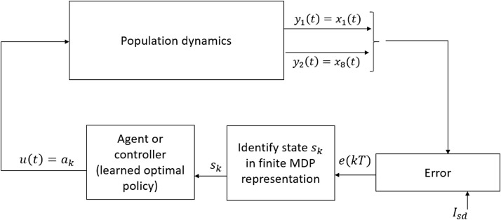
Fig. 3 shows the schematic diagram of RL-based closed-loop control of COVID-19. In the RL-based closed-loop set up, the RL-agent is capable of deriving the optimal intervention policy to drive the system in any state $s_k\in \mathcal{S}$, ${({\mathcal{S}}_i)}_{i\in I^{+}}$ to the goal state $(G_{\mathrm{s}})$ based on the converged optimal $Q$-table. Specifically, the agent assess the current state $s_k$ of the system and then imparts the action $a_k\in \mathcal{A}$ $,{({\mathcal{A}}_j)}_{j\in J^{+}}$, $J^{+}\triangleq \{1,2,\dots ,q^{\prime }\}$, $q^{\prime }=20$ which corresponds to the maximum value in the $Q$-table as determined using (29).

Fig. 3.

RL-based closed-loop control of COVID-19.

For training the RL-agent, the parameter ${\beta }_{\mathrm{w}}$ in the reward function (28) is set to ${\beta }_{\mathrm{w}}=0.5$. The choice between ${\beta }_{\mathrm{w}}=0.5$ and a higher value (e.g. ${\beta }_{\mathrm{w}}=1$) depends on the resource availability and cost affordability of the community. Compared to ${\beta }_{\mathrm{w}}=0.5$, the agent is penalized with a higher negative value when ${\beta }_{\mathrm{w}}=1$ is used. Hence, with ${\beta }_{\mathrm{w}}=1$, the agent tends to avoid actions in the high-cost set and opts only for low-cost inputs. For training the RL-agent, we iterated 20,000 (arbitrarily high) scenarios, where a scenario represents the series of transitions from an arbitrary initial state to the required terminal state $G_{\mathrm{s}}$. Furthermore, we initially assigned ${\eta }_k(s_k,a_k)=0.2$ for the first 499 scenarios and then the value of ${\eta }_k(s_k,a_k)$ is subsequently halved after every $500$th scenario. After convergence of the $Q$ table to the optimal $Q$-function, for every state $s_k$, the agent chooses an action $a_k={({\mathcal{A}}_j)}_{j\in J^{+}}$, where $j=\arg \max Q_k(s_k,·)$ (Fig. 3). Table 4 summarizes the parameters used in the $Q$-learning algorithm.

Table 4.

Parameters used in the $Q$-learning algorithm.

Parameter	Value
$k$	20,000
$T$	14 days
$\theta$	0.69
${\eta }_k$	Initialized at 0.2 then halved every 500th episode
$\delta$	0.05
${\beta }_{\mathrm{w}}$	0.5,1
$r_k$	Calculated using (28)
$ϵ$	Initialized at 1 then reduced by 0.05 every 500th episode until $ϵ=0.05$ is reached

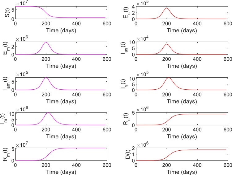
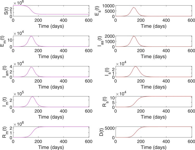
Case 1: A general population dynamics is used in this case to evaluate the performance of the RL-based closed-loop control for COVID-19. Tables 5 and 6 shows the parameter values and initial conditions used for simulating the model (1), (2), (3), (4), (5), (6), (7), (8), (9), (10), (11), (12), (13), (14), (15), (16), (17), (18), (19), (20), (21). First, the compartmental dynamics $x(t)={[S(t),E_{\mathrm{m}}(t),I_{\mathrm{am}}(t)\text{,}{I}_{\mathrm{m}}(t),R_{\mathrm{m}}(t),E_{\mathrm{s}}(t),I_{\mathrm{as}}(t),I_{\mathrm{s}}(t),R_{\mathrm{s}}(t),D(t)]}^{\mathrm{T}}$ is simulated with the initial conditions $N_0=67\times {10}^6$, $I_0=120$, and $S_0=66.99\times {10}^6$ in (1)–(21) without any control intervention (Fig. 4 ). It can be seen from Fig. 4 that the number of severely ill patients (${\mathrm{I}}_{\mathrm{s}}(t)$) who need hospitalization has peaked to $1.104\times {10}^6$ at 210th day of the epidemics. Also note that from the 98th day to 336th day, the number of severely infected is above the hospital capacity ($H=1.2\times {10}^4$) which has lead to an increased death due to COVID-19 ($1056$ on 98th day increased to $1.55\times {10}^6$ on 336th day). Similarly, indirect death due to COVID-19 has increased (0 on 98th day to $1.58\times {10}^5$ on 336th day) due to the hospital saturation. As given in (10), it can be seen that the state trajectory of $D(t)$ in Fig. 4 shows the total number of death due to direct and indirect impact of COVID.

Table 5.

Initial conditions for model (1), (2), (3), (4), (5), (6), (7), (8), (9), (10), (11), (12), (13), (14), (15).

Parameter	Initial condition (Case 1)	Initial condition (Case 2)
$N_0$	$67\times {10}^6$	2,881,053
$I_0$	$0.01H$	$1$
$S_0$	$N_0-I_0$	$N_0-I_0$
$I_{m0}$	${\mathit{pI}}_0$	${\mathit{pI}}_0$
$I_{s0}$	$(1-p)I_0$	$(1-p)I_0$
$E_{m0}$, $E_{s0}$	0	3, 0
$I_{\mathit{am}0}$, $I_{\mathit{as}0}$	0	0
$R_{m0}$, $R_{s0}$	0	0
$D_0$	0	0

Table 6.

Parameter values for model (1), (2), (3), (4), (5), (6), (7), (8), (9), (10), (11), (12), (13), (14), (15), (16), (17), (18), (19), (20), (21). For Case 1, the minimum, maximum, and typical values are shown in order [20]. For Case 2, nominal values used for simulation are shown [36], [37], [38], [40], [41].

Parameter	Values (Case 1)	Values (Case 2)
${\tau }_{\mathrm{L}}$	0.21–0.27 $({\mathrm{days}}^{-1})$ (typ. val. 1/4.2)	0.238 $({\mathrm{days}}^{-1})$
${\tau }_{\mathrm{I}}$	0.9–1.1$({\mathrm{days}}^{-1})$ (typ. val. 1)	1 $({\mathrm{days}}^{-1})$
${\lambda }_1$	0.025–0.1 $({\mathrm{days}}^{-1})$ (typ. val. 1/17)	0.1167 $({\mathrm{days}}^{-1})$
${\lambda }_2$	0.039–0.13 $({\mathrm{days}}^{-1})$ (typ. val. 1/20)	0.0583 $({\mathrm{days}}^{-1})$
$p$	0.85–0.95 $({\mathrm{days}}^{-1})$ (typ. val.0.9)	0.95 $({\mathrm{days}}^{-1})$
$m$	0.2	0.2
${\theta }_{\mathrm{c}}$	0.135–0.165 $({\mathrm{days}}^{-1})$ (typ. val. 0.15)	-
$\beta (t)$	Calculated using (16)	Calculated using (16)
${\gamma }_{\mathrm{A}}={\gamma }_{\mathrm{A}}$	Calculated using (17)	Calculated using (17)
${\mu }^{\prime }$	Calculated using (18)	Calculated using (18)
${\mu }_{\mathrm{H}}$	${10}^{-5}$$({\mathrm{days}}^{-1})$	$1\times {10}^{-6}$$({\mathrm{days}}^{-1})$
$\mu$	Calculated using (19)	Calculated using (19)
${\mu }_{\min }$	Calculated using (20)$({\mathrm{days}}^{-1})$	0.0014 $({\mathrm{days}}^{-1})$
${\mu }_{\max }$	Calculated using (21)$({\mathrm{days}}^{-1})$	0.0028 $({\mathrm{days}}^{-1})$
$\rho$	2 $({\mathrm{days}}^{-1})$	5 $({\mathrm{days}}^{-1})$
$H$	12,000	3500
$R_0$	2–3 (typ. val. 2.5)	2.1

Fig. 4.

System states without intervention for Case 1.

Note that the number of susceptibles $(S(t))$ reduces monotonically over time due to increased movement of people to the exposed or infected compartments (Fig. 4). Similarly, the number of people in recovery compartments and death compartment increases monotonically as they are terminal compartments. However, in other compartments including the severely infected $(I_{\mathrm{s}}(t))$, the number initially increases and then decreases. Hence, the value of $e(t)$, $\mathrm{kT}\le t<(k+1)T$, can be in the same range during initial and final phases of the trajectory (Fig. 4). However, the status quo of the system at these two phases are different as reflected in the trajectory of the susceptible population. Hence, different state-assignments are necessary in these two phases for the RL-agent to differentiate between the regions with similar $e(t)$ values but different $S(t)$ values. Hence, we assign $i$ states, $i=1,\dots ,10$ for $S(t)>3\times {10}^7$ and $i=11,\dots ,20$ otherwise. See Table 2 for the state assignments based on the values of $e(\mathrm{kT})$ and $S(t)$ used for Case 1. The goal state for this case is set as $G_{\mathrm{s}}\in {({\mathcal{S}}_i)}_{i\in I^{+}}$, $i=1$, which corresponds to the case where $e(\mathrm{kT})\in [0,100]$ and $S(t)>3\times {10}^7$.

Even though ${({\mathcal{S}}_i)}_{i\in I^{+}}$, $i=1$ and $i=20$ corresponds to same error range $(e(\mathrm{kT})=[0,100])$, choosing $i=1$ as target state while training the RL-agent ensures that a low infectious state is achieved by keeping the number of susceptibles $S(t)>3\times {10}^7$. This implies that the RL-agent will ensure that not all people in the susceptible compartment are eventually infected before the epidemics is contained. At this juncture, an obvious question regarding the choice of the goal state is about the possibility to set the goal state for training the RL-agent as $e(\mathrm{kT})\in [0,100]$ and $S(t)>N_0-I_{\min }$, where $I_{\min }$ represents the minimum number of infected in thousands range instead of high range of values such as $S(t)>3\times {10}^7$. Choosing a very low value of $I_{\min }$ can be achieved by implementing very strict control measures over a sufficiently long period, however, in a community with porous borders (number of infected imported cases $\rho >0$) and in case of a disease with high number of asymptomatic undetected carriers/patients, the likelihood of exponential infection spread when the restrictions are relaxed is very high. This squanders all the initial efforts taken to contain the disease and the country is more likely to see a delayed peak.

Table 3 presents the action set used for training the RL-agent. In (16), $u_1(t)$, $\mathrm{kT}\le t<(k+1)T$, corresponds to restrictions on travel and social gathering, including lockdown and social distancing. Since 100% restrictions are infeasible and not practically implementable, the action set $a_k\in \mathcal{A}$ $,{({\mathcal{A}}_j)}_{j\in J^{+}}$, $J^{+}\triangleq \{1,2,\dots ,q^{\prime }\}$, $q^{\prime }=20$ is set to $\{0,0.2,0.5,0.7,0.9\}$. Similarly, $u_2(t)$, $\mathrm{kT}\le t<(k+1)T$, which corresponds to the effect of awareness campaign and compliance of people is set to $\{0,0.3,0.5\}$ as creating awareness to achieve 100% compliance is infeasible. Finally, $u_3(t)$, $\mathrm{kT}\le t<(k+1)T$, which corresponds to the efforts taken to hospitalize infected and severely sick $I_{\mathrm{s}}(t)$ or to quarantine patients with mild infection $I_{\mathrm{m}}(t)$ is set to $\{0,0.3,0.5\}$.

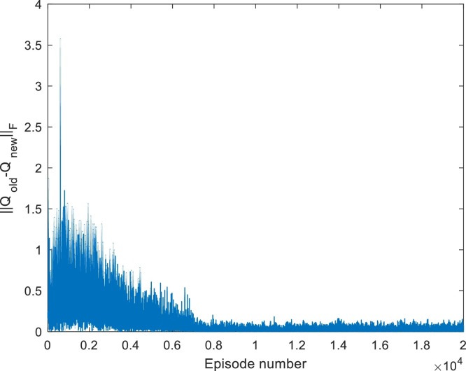
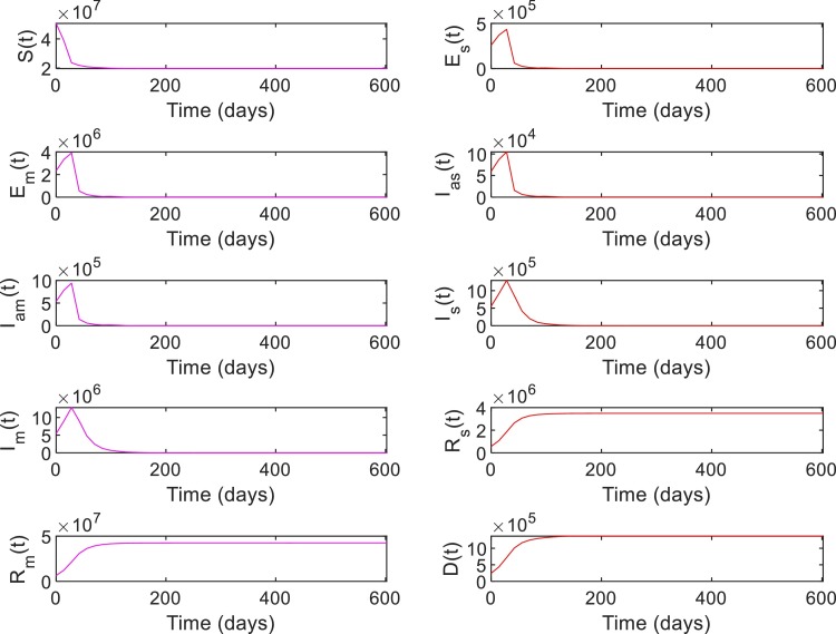
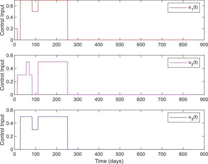
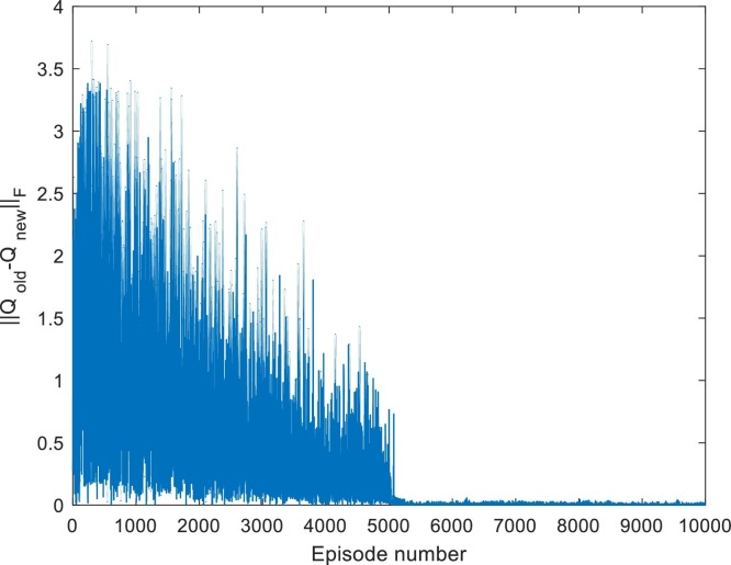
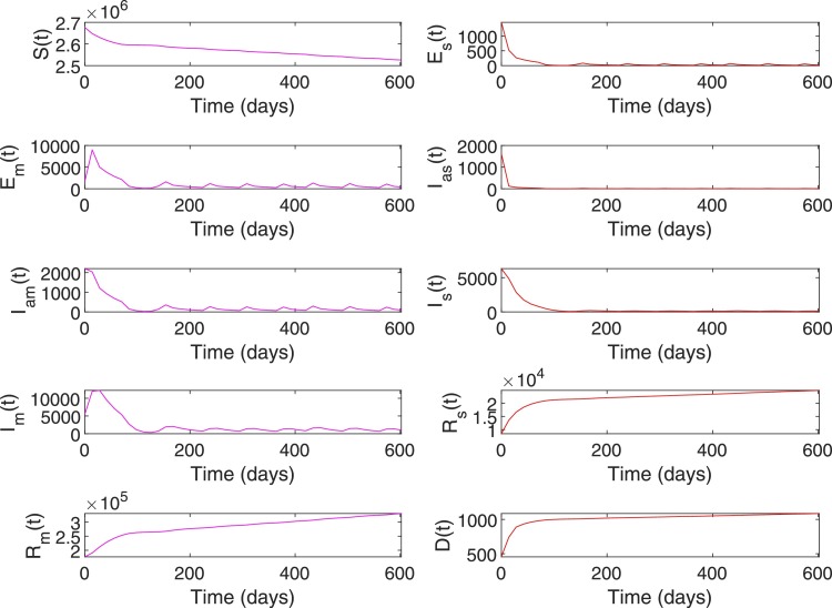
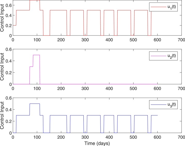
Fig. 5 shows the convergence of $Q$-table for Case 1. Figs. 6 and 7 shows the closed-loop performance of the controller with initial conditions $x(0)={[50,597,143,2,328,863,537,252\text{,}5,415,175,6,438,046,258,762,59,694,554,909,564,627,245,911]}^{\mathrm{T}}$. With $I_{\mathrm{s}0}=554,909$, this case corresponds to $I_{\mathrm{s}0}>H$ when the RL-based controller is used. As shown in Table 7 , the time duration for which $I_{\mathrm{s}}(t)\ge H$ is 238 days for no intervention and reduced to 110 days with RL-based control. Compared to the no intervention case with $D(600)=1.71\times {10}^6$, the number of death has reduced to $1.36\times {10}^6$ with RL. Note that, out of the total death at $t=600$, $2.45\times {10}^5$ corresponds to the initial value $D_0$. The peak value of $I_{\mathrm{s}}(t)$ is slightly more because the initial condition itself was $5.55\times {10}^5$ and a fraction of initial high number of population in the exposed $(E_{\mathrm{s}0})$, and asymptomatic infected $(I_{\mathrm{as}0})$ also moves to the severely infected compartment. Note that the peak value of $I_{\mathrm{s}}(t)$ represents the number of active cases at a time point, not the total number of infected. The total number of infected has reduced to $4.74\times {10}^7$ compared to the value $5.97\times {10}^7$ in the case of no intervention.

Fig. 5.

Convergence of $Q$-table for Case 1. Iterated for 20,000 episodes.

Fig. 6.

System states with RL-based control, Case 1, $I_{\mathrm{s}0}>H$, with initial conditions $x(0)={[50,597,143,2,328,863,537,252\text{,}5,415,175,6,438,046,258,762,59,694\text{,}554,909,564,627,245,911]}^{\mathrm{T}}$.

Fig. 7.

Control inputs. Case 1, $I_{\mathrm{s}0}>H$,with initial conditions $x(0)={[50,597,143,2,328,863,537,252\text{,}5,415,175,6,438,046,258,762,59,694\text{,}554,909,564,627,245,911]}^{\mathrm{T}}$.

Table 7.

Closed-loop performance, Case 1. Time $T_{\mathrm{c}}$ represents the time at which $I_{\mathrm{am}}(t)$, $I_{\mathrm{m}}(t)$, $I_{\mathrm{as}}(t)$ and $I_{\mathrm{s}}(t)$ becomes $\le 100$ for the first time.

Intervention	Time $T_{\mathrm{c}}$, $I(T_{\mathrm{c}})\le 100$	Total infected $N_0-S(T_{\mathrm{c}})$	Peak $I_{\mathrm{s}}(t)$	Time ($I_{\mathrm{s}}(t)>H$)	Death (Direct + indirect)
No intervention	434,546, 378,480	$5.97\times {10}^7$	$1.1\times {10}^6$	238 Days (98th–336th)	$1.71\times {10}^6$ ($1.55\times {10}^6+1.58\times {10}^5$)
With RL, $I_{\mathrm{s}0}>H$	196,280, 154,238	$4.74\times {10}^7$	$1.2\times {10}^6$	110 Days (98th–208th)	$1.36\times {10}^6$ ($1.2\times {10}^6+1.3\times {10}^5$)
With RL, $I_{\mathrm{s}0}<H$	110,-, 40,160	$5\times {10}^5$	$1.19\times {10}^4$	0 Days	$1.39\times {10}^4$ ($7723+6253$)

Figs. 8 and 9 shows the closed-loop performance of the RL-based controller with initial conditions $x(0)={[66,685,532,56,199,12,634,107,422\text{,}106,982,6244,1403\text{,}11,935,10,104,1783]}^{\mathrm{T}}$, i.e. with $I_{\mathrm{s}0}=11,935$, this scenario represent a case when $I_{\mathrm{s}0}<H$ when the RL-based controller is used. As shown in Table 7, the time duration for which $I_{\mathrm{s}}(t)\ge H$ is 238 days for no intervention and reduced to 0 days with RL-based control. Compared to the no intervention case with $D(600)=1.71\times {10}^6$, number of death has reduced to $1.39\times {10}^4$ with RL. Note that, out of the total death at $t=600$, $1783$ corresponds to the initial value of $D_0$. The peak value of $I_{\mathrm{s}}(t)$ has reduced to $1.19\times {10}^4$ from a value of $1.1\times {10}^6$ for no intervention and the total number of infected has reduced to $5\times {10}^5$ compared to the value $5.97\times {10}^7$ in the case of no intervention.

Fig. 8.

System states with RL-based control, Case 1. With initial conditions $x(0)={[66,685,532,56,199,12,634,107,422,106,982,6244,1403\text{,}11,935,10,104,1783]}^{\mathrm{T}}$. With $I_{\mathrm{s}}(t)=11,935$, this scenario represents a case when $I_{\mathrm{s}0}<H$.

Fig. 9.

Control inputs, Case 1, when $I_{\mathrm{s}0}<H$.

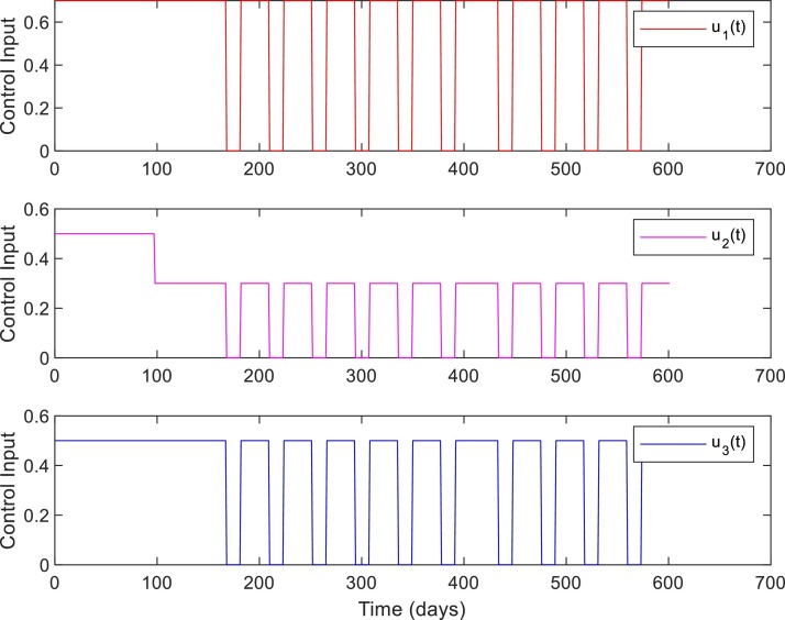
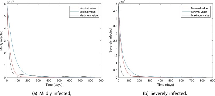
Figs. 10 and 11 show the robustness of the RL-based controller under model parameter uncertainties. The plots show the dynamics in mildly and severely infected compartments for nominal, minimum, and maximum values of model parameters. It can be seen that for all three cases the number of severely infected people ($I_{\mathrm{s}}(t)$) is below 1000 within 210 days. Moreover, $I_{\mathrm{s}}(t)\le H$ is achieved within 30, 80, and 130 days for maximum, nominal, and minimum values of model parameters.

Fig. 10.

With RL-based control, Case 1.

Fig. 11.

Control inputs for Case 1, Model parameters with nominal, minimum, and maximum values.

Comparing the control inputs for the cases $I_{\mathrm{s}0}<H$ and $I_{\mathrm{s}0}\ge H$, it can be seen that the control input for the latter case (Fig. 7) is more cost-effective. However, in the case corresponding to Fig. 9, the control input is not coming down to zero as the number of susceptible in the compartment is very high as only $5\times {10}^5$ peoples are infected. In this case, as there are imported infected cases and many unreported cases in the community, the number of cases will increase once the restrictions are relaxed. These results are in line with the effective control suggestions for earlier pandemics. In the case of an earlier influenza pandemic, studies suggested that controlling the epidemic at the predicted peak is most effective [42]. Closing too early results in the reappearing of cases if restrictions are lifted and require restrictions for a longer time period. Note that the reward function (25), (26), (27) is designed to train the controller (RL-agent) to chose control inputs that will minimize the total number of severely infected and penalize the use of high-cost control input (see Table 3). Designing a reward function that will penalize the RL-agent for variations in the control input and that can account for various delays in the system is an interesting extension of the current framework.

Considering the incubation time and delay in reporting (10–14 days), the observable output $y(t)$, $s_k=g(y(t))$, $\mathrm{kT}\le t<(k+1)T$, $k=1,2,\dots$ is sampled at every 14th day ($T=14$). To investigate the closed-loop performance of the RL-agent, we tested the RL-based controller for various sampling periods. As shown in Table 8 , for different values of $T$, the RL-based controller is able to bring down the number of severely infected to $675\pm 22$ cases by the 100th day. From Tables 7 and 8 and Figs. 10 and 11 it is clear that the proposed $Q$-learning-based controller showcase acceptable closed-loop performance. Hence, $Q$-learning algorithm is useful in deriving suitable control policies to curtail disease transmission of COVID-19. Moreover, similar to the action set of $Q$-learning framework, the control actions (e.g. lockdown) pertaining to COVID-19 are implemented in intermittently, i.e. step-wise restriction implementation and lifting. However, deep $Q$-learning or double deep $Q$-learning algorithms which involve neural network-based $Q$-functions rather than $Q$-table can be used to account for a more complex objective function that penalizes the variations in the control inputs along with other constraints in intervention and hospitalization. Moreover, the overestimation bias related to the $Q$-learning algorithm due to bootstrapping (estimate-based learning) is tackled in double deep $Q$-learning algorithm by implementing two independent $Q$-value estimators.

Table 8.

Closed-loop performance for various values of sampling period ($T$), with initial conditions $x(0)={[66,685,532,56,199,12,634,107,422,106,982,6244,1403\text{,}11,935,10,104,1783]}^{\mathrm{T}}$.

Sampling period ($T$ in days)	Number of severely ill on 100th day $I_{\mathrm{s}}(100)$
1	705
5	660
8	666
10	660
14	704
20	659

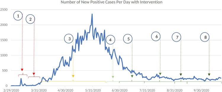
Case 2: In this case, the COVID-19 disease transmission data of Qatar is used to conduct various scenario analysis. Comparatively, the population in Qatar ($2.88\times {10}^6$) is far less than that of Case 1 ($6.7\times {10}^7$). Fig. 12 shows the number of infected cases reported per day in Qatar from 29th February to 22nd October. The first case ($I_0=1$) is that of a 36-year-old male who traveled to Qatar during the repatriation of Qatari nationals stranded in Iran. Table 5 shows the initial conditions used for our simulations and the value of $E_{\mathrm{m}0}$ is set 3 [36]. The majority of the population in Qatar are young expatriates and hence the value of $R_0$, severity of the disease, and mortality rate associated with COVID-19 in Qatar is estimated to be lesser than many other countries [36], [40], [41]. In [41], it is reported that, the case fatality rate in Qatar is 1.4 out of 1000, hence ${\mu }_{\min }=0.0014$ is used for Case 2. Active disease mitigation policies of the government and appropriate public health response of a well-resourced population has also played a key role in bringing down the total number of COVID-19 infections and associated death in Qatar [41]. Various restriction and relaxation phases implemented in Qatar are marked in Fig. 12 as (1)–(8). As mentioned in Table 9 , step by step lifting of restrictions started on June 15th. Number of new positive cases on June 15th is 1274 (Fig. 12) and number of active cases is 22,119. In the month of October, the number of active positive cases oscillated between 2764 to 2906. As of October 22nd, the total number of infection and death are 130,462 and 228, respectively. Note that, the number of severely infected (active acute cases + active ICU cases) is above 100 cases as of October 22nd (see Table 11).

Fig. 12.

Number of infected per day with intervention decisions by Qatar government. Data from 29th February to 22nd October is shown.

Table 9.

Time line of various interventions and relaxation implemented in Qatar. HC: health care.

SN	Date	Intervention
(1)	March 9th	Passengers from 14 countries banned. Only, entry of passengers with Qatar residence permit allowed subject to COVID-19 protocols.
	March 10th	Schools and colleges closed.
	March 13th	Theatres, wedding gatherings, children play area, gyms suspended.
	March 14th	Travel ban added for 3 more countries taking total to 17 countries.
	March 15th	All public transportation closed.
(2)	March 17th	All commercial complexes, shopping centers except pharmacy and food outlets closed for 14 days.
	March 18th	All incoming flights suspended.
	March 22nd	Physical presence of employees limited to 20% employees and remote operation for rest of employees in government offices.
	March 27th	Distance learning started.
(3)	April 2nd	Employers directed to allow physical presence of 20% employees and remote operation of 80% employees.
(4)	June 15th	Phase 1: Allowed limited opening (mosque, park, outdoor sports, shops, malls), essential flying out of Qatar, 40% capacity at private HC facility.
(5)	July 1st	Phase 2: Allowed gathering of $<=5$ people, 60% capacity at private HC facility, restricted capacity and hours at leisure and business areas, and 50% employees at workplace.
(6)	July 28th	Phase 3: Allowed gathering of $<=10$ people in door and $<=30$ outdoor, 50% capacity at leisure and business areas, and 80% employees at workplace. From 1st of August, Qatar permitted exceptional entry of residence stuck abroad.
(7)	September 1st	Phase 4 (Part 1): Allowed all gathering with precautions, expanded inbound flights, metro, bus, 100% capacity at private HC.
(8)	September 15th	Phase 4 (Part 2): Allowed 80% employees at workspace and 30% capacity at restaurants and food courts.

Table 11.

Closed-loop performance, Case 2. Time $T_{\mathrm{c}}$ represents the time at which $I_{\mathrm{am}}(t)$, $I_{\mathrm{m}}(t)$, $I_{\mathrm{as}}(t)$, and $I_{\mathrm{s}}(t)$ becomes $\le 100$ for the first time.

Intervention	Time $T_{\mathrm{c}}$, $I(T_{\mathrm{c}})\le 100$	Total infected $N_0-S(T_{\mathrm{c}})$	Peak $I_{\mathrm{s}}(t)$	Time ($I_{\mathrm{s}}(t)>H$)	Death (Direct + indirect)
Government intervention	-,-,-,-	$1.30\times {10}^5$	2190	0 Days	228 (228 + 0)
No intervention	259,329, 217,301	$2.36\times {10}^6$	$2.75\times {10}^4$	115 Days (105th–220th)	5605 (5263 + 342)
With RL, $I_{\mathrm{s}0}>H$	211,-,141,237,	$3.41\times {10}^5$	6323	36 Days	1065 (777 + 288)
With RL, $I_{\mathrm{s}0}<H$	169,$-$134,211,197	$1.01\times {10}^5$	1174	0 Days	121 (121 + 0)

The parameter values used for simulating the disease transmission dynamics in Qatar are given in Table 6. Compared to the no intervention case, the number of infected cases and death with government imposed restrictions are significantly less. See Tables 9 and 11 and Figs. 12 and 13.

Fig. 13.

System states without intervention for Case 2.

Next, the use of an RL-based controller for the scenarios $I_{\mathrm{s}}(t)>H$ and $I_{\mathrm{s}}(t)<H$ and a case wherein a disturbance due to the import of infected cases are analyzed. Similar to Case 1, to train RL-agent, we assign $i$ states, $i=1,\dots ,10$ for $S(t)>1.2\times {10}^6$ and $i=11,\dots ,20$ otherwise. See Table 10 for the state assignments based on the values of $e(\mathrm{kT})$ and $S(t)$ used for Case 2. For this case, we iterated for 10,000 scenarios with the goal state $G_{\mathrm{s}}=s_1$, which corresponds to the case where $e(\mathrm{kT})\in [0,100]$ and $S(t)>1.2\times {10}^6$. One of the important concerns pertaining to COVID-19 is the possibility of hospital saturation which will lead to increased indirect death due to COVID-19. Qatar government responded rapidly to the need for increased hospital capacity. Apart from arranging 37,000 isolation beds and 12,500 quarantine beds, the government has set up 3000 acute care beds and 700 intensive care beds [38], [43]. Hence, the hospital saturation capacity $H$ which is related to severely sick is set to $3500$ in (25) while training the RL-agent. The action set $a_k\in \mathcal{A}$, ${({\mathcal{A}}_j)}_{j\in J^{+}}$, and the cost assignments $c_{a_k}$ for assessing the reward (27) is given in Table 3. Fig. 14 shows the convergence of the $Q$-table for Case 2.

Table 10.

State assignment based on $e(t)$ and $S(t)$, ${({\mathcal{S}}_i)}_{i\in I^{+}}$, where $I^{+}\triangleq \{1,2,\dots ,q\}$, $q=20$.

Case 2
$S(t)>1.2\times {10}^6$		$S(t)<=1.2\times {10}^6$
$i$th state $(s_k)$ in ${\mathcal{S}}_i$	$e(\mathit{kT})$	$i$th state $(s_k)$ in ${\mathcal{S}}_i$	$e(\mathit{kT})$
$1$	[0, 100]	$11$	[40,000, $\infty$]
$2$	(100, 200]	$12$	(30,000, 40,000]
$3$	(200, 500]	$13$	(20,000, 30,000]
$4$	(500, 1000]	$14$	(10,000, 20,000]
$5$	(1000, 5000]	$15$	(5000, 10,000]
$6$	(5000, 10,000]	$16$	(1000, 5000]
$7$	(10,000, 20,000]	$17$	(500, 1000]
$8$	(20,000, 30,000]	$18$	(200, 500]
$9$	(30,000, 40,000]	$19$	(100, 200]
$10$	(40,000, $\infty$]	$20$	(0, 100]

Fig. 14.

Convergence of $Q$-table for Case 2. Iterated for 10,000 episodes.

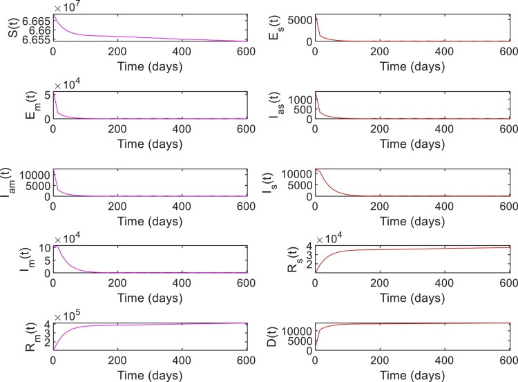
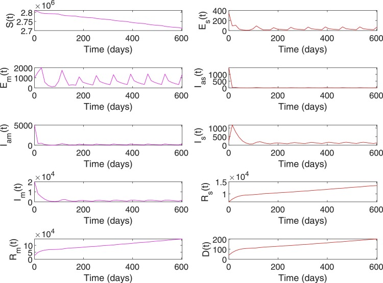
Note that, with appropriate public health response and relatively young expat population with lower risk of severe COVID-19 illness, Qatar never had severely infected cases above $H$. However, as shown in Fig. 13, the scenario $I_{\mathrm{s}}(t)\ge H$ is valid with no intervention. The initial condition for the case $I_{\mathrm{s}0}>H$ is set be $x(0)={[2,676,451,1741,2206,5518\text{,}176,817,1460,1616\text{,}6323,8466,455]}^{\mathrm{T}}$. Figs. 15 and 16 show the simulation plots of system states and control input for $I_{\mathrm{s}0}=6323>H$. The RL-based controller derives control input to bring down the cases within the range [0,100] in 117 days of intervention, whereas without intervention it took 179 days for the same. As shown in Table 11 , both the direct and indirect death due to COVID-19 is reduced to 777 and 288 when compared to 5263 and 342 in the case of no intervention. Moreover, when $I_{\mathrm{s}}(t)$ stays above $H$ for 115 days in the case of no intervention, it is reduced to 36 days in the case with an RL-based controller.

Fig. 15.

System states, Case 2. $I_{\mathrm{s}0}>H$, $x(0)={[2,676,451,1741,2206,5518,176,817,1460,1616,6323,8466,455]}^{\mathrm{T}}$.

Fig. 16.

Control input, Case 2. $I_{\mathrm{s}0}>H$, $x(0)={[2,676,451,1741,2206,5518,176,817,1460,1616,6323,8466,455]}^{\mathrm{T}}$.

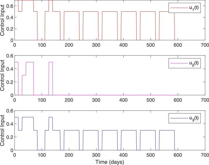
Figs. 17 and 18 show the closed-loop performance of the controller with initial conditions $x(0)={[2,810,387,1000,4991,19,965,26,750,350,1493,240,6687,40]}^{\mathrm{T}}$. This set of initial conditions is from the COVID-19 data of Qatar on June 1st and it corresponds to the scenario $I_{\mathrm{s}0}<H$ with $I_{\mathrm{s}0}=240$. As shown in Fig. 17, by 600 days from June 1st, direct and indirect deaths are 202 and 0, respectively. As given in Table 11, on October 22nd, the total number of infected and deaths with government intervention is $1.30\times {10}^5$ and 228 and with RL-based control is $1.01\times {10}^5$ and 121. Note that October 22nd corresponds to 144th day in Fig. 17. With RL-based control, the number of susceptibles is more than $2.72\times {10}^6$ ($>94\%$) throughout. Since, a very low percentage of the total population is infected, the likelihood of seeing secondary waves when control is lifted is very high. It can be seen from Figs. 17 and 18 that whenever control input goes to zero slight increase in the number of infected is resulted and hence the control is increased to keep the active number of infected near 100. Note that as of October 22nd, the active number of cases with government intervention is 2484 (mild) and 422 (severe).

Fig. 17.

System states, Case 2. $I_{\mathrm{s}0}<H$, $x(0)={[2,810,387,1000,4991,19,965,26,750,350,1493,240,6687,40]}^{\mathrm{T}}$.

Fig. 18.

Control input, Case 2. $I_{\mathrm{s}0}<H$, $x(0)={[2,810,387,1000,4991,19,965,26,750,350,1493,240,6687,40]}^{\mathrm{T}}$.

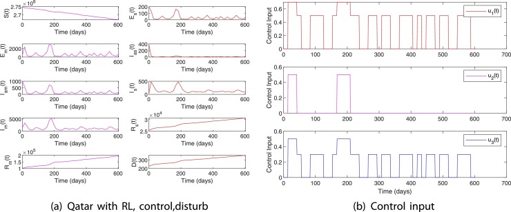
Next, we simulate a scenario with disturbance. Social gatherings and other behavioral strategies that are not in compliance with the COVID-19 mitigation protocols can considerably increase the transmission rate $\beta (t)$. The import of infected cases through international airports can also increase the infection rate in society. Such changes can be modeled as a disturbance that contributes to a sudden change in the value of $\beta (t)$. Qatar is a country with considerable international traffic and on average the Doha airport was handling 100,000 passengers per day before the pandemic [44]. However, due to COVID-19 restrictions only around 20% of the regular traffic is expected to arrive in Qatar. Out of these passengers a small percentage can be infected despite the strict screening strategies including the testing and quarantining protocols followed currently. Hence, a per day import of 5 infected cases ($\rho =5$) is used for the nominal model for Case 2. However, completely lifting travel restrictions can increase the number of imported infected cases.

Fig. 19 shows the performance of the RL-based closed-loop controller when a disturbance in the form of an increase in $\rho$ is introduced to the system. For this scenario, the initial condition $x(0)={[2,749,893,500,1000,1484,101,860\text{,}200,384,38,25,466,228]}^{\mathrm{T}}$ and $R_0=1.68$ is used [41]. This initial condition corresponds to the COVID-19 infection data in Qatar on October 22nd. Starting from October 22nd, a disturbance of $\rho =500$ (${\mathrm{days}}^{-1}$) is applied on the 150th day and maintained for 4 weeks. This disturbance model a scenario wherein 500 infected cases are imported per day due to relaxing all restrictions on international travel. It can be seen from Fig. 19 that the control input is increased during the time of disturbance to limit the total number of infected and death to 211,053 and 352, respectively. Also, note that the import of a lesser number ($<100$) of infected cases does not significantly influence the dynamics of the COVID-19 in the society. The results of this simulation study imply that it is imperative to limit the number of imported cases per day below 100 per day by implementing testing and screening strategies as it is done currently until the number of cases is reduced worldwide or a protective vaccine is available.

Fig. 19.

Case 2 with disturbance. $x(0)={[2,749,893,500,1000,1484,101,860\text{,}200,384,38,25,466,228]}^{\mathrm{T}}$, $R_0=1.68$, $\rho =500$ per day 150 days after October 22nd for 4 weeks.

In general, simulation results for Case 1 and Case 2 show that even though the relaxation of control measures can be started when the peak declines, complete relaxation is advised only if the number of active cases falls below 100 and a significant proportion of the total population is infected (Fig. 7). If the total number of active cases is above 100 and/or the number of susceptibles is significantly high, it is recommended to exercise 50% control on overall interactions of the infected (detected and undetected) which includes maintaining social distancing, sanitizing contaminated surfaces, and isolating detected cases. International travel can be allowed by following COVID-19 protocols and continuing screening and testing of the passengers to keep the number of imported cases to a minimum.

4. Conclusions and future work

In this paper, we have demonstrated the use of an RL-based learning framework for the closed-loop control of an epidemiological system, given a set of infectious disease characteristics in a society with certain socio-economic and healthcare characteristics and constraints. Simulation results show that the RL-based controller can achieve the desired goal state with acceptable performance in case of disturbances. Incorporating real-time regression models to update the parameters of the simulation model to match the real-time disease transmission dynamics can be a useful extension of this work.

Author contribution statement

Conceptualization – Nader Meskin and Tamer Kattab

Writing and original draft preparation – Regina Padmanabhan

Reviewed and edited by – Nader Meskin, Tamer Kattab, Mujahed Shraim, and Mohammed Al-Hitmi

All authors have read and agreed to the published version of the manuscript.

Conflict of interest

The authors declare no conflict of interest.

References

- 1.Rajaei A., Vahidi-Moghaddam A., Chizfahm A., Sharifi M. Control of malaria outbreak using a non-linear robust strategy with adaptive gains. IET Control Theory Appl. 2019;13(14):2308–2317. [Google Scholar]
- 2.Sharifi M., Moradi H. Nonlinear robust adaptive sliding mode control of influenza epidemic in the presence of uncertainty. J. Process Control. 2017;56:48–57. [Google Scholar]
- 3.Momoh A.A., F“ugenschuh A. Optimal control of intervention strategies and cost effectiveness analysis for a zika virus model. Oper. Res. Health Care. 2018;18:99–111. [Google Scholar]
- 4.WHO . 2016. Anticipating Emerging Infectious Disease Epidemics.https://apps.who.int/iris/bitstream/handle/10665/252646/WHO-OHE-PED-2016.2-eng.pdf [Google Scholar]
- 5.Chakraborty A., Sazzad H., Hossain M., Islam M., Parveen S., Husain M., Banu S., Podder G., Afroj S., Rollin P., et al. Evolving epidemiology of nipah virus infection in bangladesh: evidence from outbreaks during 2010–2011. Epidemiol. Infect. 2016;144(2):371–380. doi: 10.1017/S0950268815001314. [DOI] [PMC free article] [PubMed] [Google Scholar]
- 6.Izadi M.T., Buckeridge D.L. Proceedings of the National Conference on Artificial Intelligence, vol. 22, no. 2. AAAI Press; MIT Press; Menlo Park, CA; Cambridge, MA; London: 2007. Optimizing anthrax outbreak detection using reinforcement learning; p. 1781. 1999. [Google Scholar]
- 7.Duan W., Fan Z., Zhang P., Guo G., Qiu X. Mathematical and computational approaches to epidemic modeling: a comprehensive review. Front. Comput. Sci. 2015;9(5):806–826. doi: 10.1007/s11704-014-3369-2. [DOI] [PMC free article] [PubMed] [Google Scholar]
- 8.Archie E.A., Luikart G., Ezenwa V.O. Infecting epidemiology with genetics: a new frontier in disease ecology. Trends Ecol. Evol. 2009;24(1):21–30. doi: 10.1016/j.tree.2008.08.008. [DOI] [PubMed] [Google Scholar]
- 9.of the Madrid O.C., Reiz A.N., Sagasti F.M., González M.Á., Malpica A.B., Benítez J.C.M., Cabrera M.N., del Pino Ramírez Á., Perdomo J.M.G., Alonso J.P., et al. Big data and machine learning in critical care: opportunities for collaborative research. Med. Intensiva. 2019;43(1):52–57. doi: 10.1016/j.medin.2018.06.002. [DOI] [PubMed] [Google Scholar]
- 10.Comissiong D., Sooknanan J. A review of the use of optimal control in social models. Int. J. Dyn. Control. 2018;6(4):1841–1846. [Google Scholar]
- 11.Ibeas A., De La Sen M., Alonso-Quesada S. Robust sliding control of SEIR epidemic models. Math. Probl. Eng. 2014;2014 [Google Scholar]
- 12.Wang X., Shen M., Xiao Y., Rong L. Optimal control and cost-effectiveness analysis of a zika virus infection model with comprehensive interventions. Appl. Math. Comput. 2019;359:165–185. [Google Scholar]
- 13.Laguzet L., Turinici G. 2014. Globally Optimal Vaccination Policies in the SIR Model: Smoothness of the Value Function and Uniqueness of the Optimal Strategies. [Google Scholar]
- 14.Yi N., Zhang Q., Mao K., Yang D., Li Q. Analysis and control of an SEIR epidemic system with nonlinear transmission rate. Math. Comput. Model. 2009;50(9–10):1498–1513. doi: 10.1016/j.mcm.2009.07.014. [DOI] [PMC free article] [PubMed] [Google Scholar]
- 15.Makhoul M., Ayoub H.H., Chemaitelly H., Seedat S., Mumtaz G.R., Al-Omari S., Abu-Raddad L.J. Epidemiological impact of SARS-CoV-2 vaccination: mathematical modeling analyses. medRxiv. 2020 doi: 10.3390/vaccines8040668. [DOI] [PMC free article] [PubMed] [Google Scholar]
- 16.Hellewell J., Abbott S., Gimma A., Bosse N.I., Jarvis C.I., Russell T.W., Munday J.D., Kucharski A.J., Edmunds W.J., Sun F., et al. Feasibility of controlling COVID-19 outbreaks by isolation of cases and contacts. Lancet Global Health. 2020 doi: 10.1016/S2214-109X(20)30074-7. [DOI] [PMC free article] [PubMed] [Google Scholar]
- 17.Tang B., Wang X., Li Q., Bragazzi N.L., Tang S., Xiao Y., Wu J. Estimation of the transmission risk of the 2019-nCoV and its implication for public health interventions. J. Clin. Med. 2020;9(2):462. doi: 10.3390/jcm9020462. [DOI] [PMC free article] [PubMed] [Google Scholar]
- 18.Tang B., Bragazzi N.L., Li Q., Tang S., Xiao Y., Wu J. An updated estimation of the risk of transmission of the novel coronavirus (2019-nCov) Infect. Dis. Model. 2020;5:248–255. doi: 10.1016/j.idm.2020.02.001. [DOI] [PMC free article] [PubMed] [Google Scholar]
- 19.B”arwolff G. Mathematical modeling and simulation of the COVID-19 pandemic. Systems. 2020;8(3):24. [Google Scholar]
- 20.Djidjou-Demasse R., Michalakis Y., Choisy M., Sofonea M.T., Alizon S. Optimal COVID-19 epidemic control until vaccine deployment. medRxiv. 2020 [Google Scholar]
- 21.Ames A.D., Molnár T.G., Singletary A.W., Orosz G. Safety-critical control of active interventions for COVID-19 mitigation. IEEE Access. 2020 doi: 10.1109/ACCESS.2020.3029558. [DOI] [PMC free article] [PubMed] [Google Scholar]
- 22.Shortreed S.M., Laber E., Lizotte D.J., Stroup T.S., Pineau J., Murphy S.A. Informing sequential clinical decision-making through reinforcement learning: an empirical study. Mach. Learn. 2011;84(1–2):109–136. doi: 10.1007/s10994-010-5229-0. [DOI] [PMC free article] [PubMed] [Google Scholar]
- 23.Martín-Guerrero J.D., Gomez F., Soria-Olivas E., Schmidhuber J., Climente-Martí M., Jiménez-Torres N.V. A reinforcement learning approach for individualizing erythropoietin dosages in hemodialysis patients. Expert Syst. Appl. 2009;36(6):9737–9742. [Google Scholar]
- 24.Padmanabhan R., Meskin N., Haddad W.M. Reinforcement learning-based control of drug dosing for cancer chemotherapy treatment. Math. Biosci. 2017;293:11–20. doi: 10.1016/j.mbs.2017.08.004. [DOI] [PubMed] [Google Scholar]
- 25.Zhao Y., Zeng D., Socinski M.A., Kosorok M.R. Reinforcement learning strategies for clinical trials in nonsmall cell lung cancer. Biometrics. 2011;67(4):1422–1433. doi: 10.1111/j.1541-0420.2011.01572.x. [DOI] [PMC free article] [PubMed] [Google Scholar]
- 26.Yazdjerdi P., Meskin N., Al-Naemi M., Al Moustafa A.-E., Kovács L. Reinforcement learning-based control of tumor growth under anti-angiogenic therapy. Comput. Methods Programs Biomed. 2019;173:15–26. doi: 10.1016/j.cmpb.2019.03.004. [DOI] [PubMed] [Google Scholar]
- 27.Padmanabhan R., Meskin N., Haddad W.M. Closed-loop control of anesthesia and mean arterial pressure using reinforcement learning. Biomed. Signal Process. Control. 2015;22:54–64. [Google Scholar]
- 28.Wiens J., Shenoy E.S. Machine learning for healthcare: on the verge of a major shift in healthcare epidemiology. Clin. Infect. Dis. 2018;66(1):149–153. doi: 10.1093/cid/cix731. [DOI] [PMC free article] [PubMed] [Google Scholar]
- 29.Kreatsoulas C., Subramanian S. Machine learning in social epidemiology: learning from experience. SSM-Popul. Health. 2018;4:347. doi: 10.1016/j.ssmph.2018.03.007. [DOI] [PMC free article] [PubMed] [Google Scholar]
- 30.Watkins C.J.C.H., Dayan P. Q-learning. Mach. Learn. J. 1992;8(3):279–292. [Google Scholar]
- 31.Vrabie D., Vamvoudakis K.G., Lewis F.L. Institution of Engineering and Technology; London, UK: 2013. Optimal Adaptive Control and Differential Games by Reinforcement Learning Principle. [Google Scholar]
- 32.Sutton R.S., Barto A.G. MIT Press; Cambridge, MA: 1998. Reinforcement Learning: An Introduction. [Google Scholar]
- 33.Bertsekas D.P., Tsitsiklis J.N. Athena Scientific; MA: 1996. Neuro-Dynamic Programming. [Google Scholar]
- 34.Barto A.G., Sutton R.S., Anderson C.W. Neuronlike adaptive elements that can solve difficult learning control problems. IEEE Trans. Syst. Man Cybern. 1983;13:834–846. [Google Scholar]
- 35.Ghanam R., Boone E., Abdel-Salam A.-S. COVID-19: SEIRD model for Qatar COVID-19 outbreak. Lett. Biomath. 2020 [Google Scholar]
- 36.Fahmy A.E., Eldesouky M.M., Mohamed A.S. Epidemic analysis of COVID-19 in Egypt, Qatar and Saudi Arabia using the generalized SEIR model. medRxiv. 2020 [Google Scholar]
- 37.data.gov.qa . 2020. Qatar Open Data Portal.https://www.data.gov.qa/explore/dataset/covid-19-cases-in-qatar [Google Scholar]
- 38.of Public Health M. 2020. Coronavirus Disease (COVID-19)https://www.moph.gov.qa/english/mediacenter/News/Pages/default.aspx [Google Scholar]
- 39.Wikipedia . 2020. COVID-19 Pandemic in Qatar.https://en.wikipedia.org/wiki/COVID-19-pandemic-in-Qatar [Google Scholar]
- 40.Planning and statistics authority . 2017. Births and Deaths in State of Qatar.https://www.psa.gov.qa/en/statistics/Statistical [Google Scholar]
- 41.Abu-Raddad L.J., Chemaitelly H., Ayoub H.H., Al Kanaani Z., Al Khal A., Al Kuwari E., Butt A.A., Coyle P., Latif A.N., Owen R.C., et al. Characterizing the Qatar advanced-phase SARS-CoV-2 epidemic. medRxiv. 2020 doi: 10.1038/s41598-021-85428-7. [DOI] [PMC free article] [PubMed] [Google Scholar]
- 42.Modchang C., Iamsirithaworn S., Auewarakul P., Triampo W. A modeling study of school closure to reduce influenza transmission: a case study of an influenza A (H1N1) outbreak in a private Thai school. Math. Comput. Model. 2012;55(3–4):1021–1033. [Google Scholar]
- 43.Al Khal A., Al-Kaabi S., Checketts R.J., et al. Qatar's response to COVID-19 pandemic. Heart Views. 2020;21(3):129. doi: 10.4103/HEARTVIEWS.HEARTVIEWS_161_20. [DOI] [PMC free article] [PubMed] [Google Scholar]
- 44.QCCA . 2019. Qatar Civil Aviation Authority, Open Data, Air Transport Data.https://www.caa.gov.qa/en-us/Open [Google Scholar]