MRI Manufacturer Shift and Adaptation: Increasing the Generalizability of Deep Learning Segmentation for MR Images Acquired with Different Scanners

Abstract

Purpose

To quantitatively evaluate the generalizability of a deep learning segmentation tool to MRI data from scanners of different MRI manufacturers and to improve the cross-manufacturer performance by using a manufacturer-adaptation strategy.

Materials and Methods

This retrospective study included 150 cine MRI datasets from three MRI manufacturers, acquired between 2017 and 2018 (n = 50 for manufacturer 1, manufacturer 2, and manufacturer 3). Three convolutional neural networks (CNNs) were trained to segment the left ventricle (LV), using datasets exclusively from images from a single manufacturer. A generative adversarial network (GAN) was trained to adapt the input image before segmentation. The LV segmentation performance, end-diastolic volume (EDV), end-systolic volume (ESV), LV mass, and LV ejection fraction (LVEF) were evaluated before and after manufacturer adaptation. Paired Wilcoxon signed rank tests were performed.

Results

The segmentation CNNs exhibited a significant performance drop when applied to datasets from different manufacturers (Dice reduced from 89.7% ± 2.3 [standard deviation] to 68.7% ± 10.8, P < .05, from 90.6% ± 2.1 to 59.5% ± 13.3, P < .05, from 89.2% ± 2.3 to 64.1% ± 12.0, P < .05, for manufacturer 1, 2, and 3, respectively). After manufacturer adaptation, the segmentation performance was significantly improved (from 68.7% ± 10.8 to 84.3% ± 6.2, P < .05, from 72.4% ± 10.2 to 85.7% ± 6.5, P < .05, for manufacturer 2 and 3, respectively). Quantitative LV function parameters were also significantly improved. For LVEF, the manufacturer adaptation increased the Pearson correlation from 0.005 to 0.89 for manufacturer 2 and from 0.77 to 0.94 for manufacturer 3.

Conclusion

A segmentation CNN well trained on datasets from one MRI manufacturer may not generalize well to datasets from other manufacturers. The proposed manufacturer adaptation can largely improve the generalizability of a deep learning segmentation tool without additional annotation.

Supplemental material is available for this article.

© RSNA, 2020

Summary

A deep learning segmentation tool developed by using MRI data from one MRI scanner may not generalize well to MRI data from another MRI manufacturer’s scanner; the authors propose an MRI manufacturer adaptation method to improve the generalizability of a deep learning segmentation tool without additional manual annotation.

Key Points

• ■ A well-trained deep learning MRI segmentation tool exhibited significantly degraded performance when applied to data acquired from an MRI scanner of a different manufacturer.

• ■ The generalizability of deep learning segmentation can be improved by aggregating annotated training data from different manufacturer scanners.

• ■ The generalizability of deep learning segmentation can be improved by applying the proposed manufacturer adaptation to other manufacturer data without need of new annotation.

Introduction

MRI is a versatile, noninvasive imaging technique to examine the soft tissue with fine resolution and excellent contrast (1). With advancement in MRI physics, improvements have been made in visualizing organs in an accurate and comprehensive manner. Meanwhile, the rapid development of artificial intelligence techniques enables fast, accurate, and objective analysis of MR images (2,3). Today, deep learning convolutional neural networks (CNNs) are the state of the art for many MR image analysis tasks, especially for organ segmentation that is traditionally performed by expert radiologists. There is accumulating evidence that CNNs can achieve expert-level performance in many classic MRI segmentation problems, such as on brain, heart, and tumors (4–7). CNN tools may save tedious manual work and avoid user subjectivity, further enhancing the value of MRI. However, before the widespread adoption of CNN tools in clinical practice, there is a question that must be addressed: Would the CNN work on the data from my MRI machine at my center?

As suggested by its name, a deep learning CNN is a learning-based method (8). At the training stage, a CNN is given a large amount of training data including the original MR images and their manual segmentations. The CNN learns its internal parameters (up to millions) from the training data, such that the input image can be mapped to the known segmentation. It is critical to be as accurate as possible during the training stage. At the deployment stage, the trained CNN is applied to an “unseen” image and uses the trained parameters to predict its segmentation. The generalizability of the trained CNN to an unseen dataset, therefore, is of utmost importance for its practical deployment.

Although many previous studies have tested their CNNs on an independent testing dataset, the generalization problem still persists for MRI data. CNN is a statistical method, which learns the statistics of the training data under the identical independent distribution (IID) assumption (9), which implies that the trained CNN is supposed to work on data with identical or similar distributions. However, MR images are predisposed to statistical shift, caused by differences in sequences, scanner manufacturers, and centers. Manufacturer differences are a major cause of statistical shift, as different MRI scanners produce images of different characteristics related to manufacturer-specific MRI physics (10). When the statistical distribution shifts, a well-trained CNN may fail. The unsatisfactory generalization of CNNs across MRI data from different manufacturers has been reported previously (11) and noted in expert reviews (12,13).

Intuitively, we can include as much training data as possible from different manufacturers to learn an all-inclusive statistical distribution (4,14,15). However, manual annotation of large MRI datasets for every new dataset to retrain the CNN is exceedingly expensive and practically impossible. A more feasible solution is to transform the statistics of the input data to that of the training data, such that it meets the IID assumption. In the context of deep learning, this equates to translating images from the “target domain” to the “source domain” (16). Study of generative adversarial networks (GANs) is a prominent research area that focuses on the generation of new data with the same statistics as the training set (17,18). Generation of statistically similar datasets provides a possibility to tackle the manufacturer shift problem without additional annotations.

This study aims to address the MRI manufacturer shift problem that hampers the practical utilization of deep learning segmentation tools and present a solution by GAN-based manufacturer adaptation. We use the left ventricular (LV) segmentation from cine MRI as a representative case.

Materials and Methods

Data from Multiple Manufacturers

Three MRI datasets were retrospectively included in this study. The use of the MRI data was approved by the local institutional review board and written informed consent to use the data was obtained from all patients. All data were anonymized prior to the analysis. Cine MRI data were collected from two centers, from three major MRI scanner manufacturers. The manufacturers included three major players in the field of MRI: GE, Philips, Siemens (in no particular order). For each scanner manufacturer, 50 consecutive patients referred for cardiovascular MRI examination for clinical reasons between 2017 and 2018 were included. The datasets collected from each scanner were called manufacturer 1, manufacturer 2, and manufacturer 3.

Clinical indications included myocardial infarction, hypertrophy, and dilated cardiomyopathy for reference to the MRI examination. In some cases, there were no cardiovascular findings at MRI. The basic patient information is as follows: mean age, 57 years ± 20 standard deviation (58% male); 62 years ± 23 (48% male); and 58 years ± 23 (54% male), for manufacturer 1, manufacturer 2, and manufacturer 3, respectively.

MR Image Acquisition for Different MRI Machine Manufacturer Datasets

The typical cine MRI parameters for each of the three MRI machine manufacturers are reported in Table 1.

Table 1:

Specifications of Cine MRI Datasets Acquired from Scanners of Different Manufacturers

Manual Annotation

Cine MR images were manually analyzed by two experienced observers (L.H., S.G.) with 7 and 5 years experience in cardiac MRI, respectively. The myocardium endocardial and epicardial borders were manually annotated using the MASS software (research version, Leiden University Medical Center, Leiden, the Netherlands. For all datasets, the cine MR image frames close to the end-diastolic and end-systolic phases were annotated, with both endocardial and epicardial contours manually drawn.

Training and Testing Datasets

Datasets from each manufacturer were randomly divided by 2:1 ratio for training and testing (33 and 17 patients). The division was based on patients such that the frames in training and testing sets were not correlated. As annotation was used as the reference standard for both training and testing purposes, the annotated frames were only used for development and evaluation. The number of total and annotated cine frames for training and testing is reported in Table 1. The training data were used to build up the segmentation CNN and the GAN adaptor. The testing data were used to evaluate the segmentation and adaptation performance.

LV Segmentation by U-Net

U-Net is an established CNN architecture for medical image segmentation (7). It consists of a contracting path that extracts image features and an expanding path that upsamples features and convolutes them into a segmentation map. Given the training set of MR images and their manual segmentation, the U-Net learns an image-to-segmentation mapping. Multiple studies have demonstrated its excellent performance on the segmentation of cine MR images (4,15,19).

The architecture of the LV segmentation U-Net is shown in Figure E1 (supplement). Data augmentation was performed by applying random transformations to the original training image, including rotation, rescaling, and translation. The same augmentation was applied to the label image. Each pair of training image and label image was augmented to 30 pairs for training the U-Net.

To evaluate the manufacturer shift problem, we trained three manufacturer-specific U-Nets, named U-Net 1, U-Net 2, and U-Net 3, using the training datasets from manufacturer 1, manufacturer 2, and manufacturer 3, respectively. All images were first rescaled to the same in-plane resolution of 1.5 × 1.5 mm. Cine MR and label images were cropped at the center to a size of 192 × 192 pixels. We used an Adam optimizer with a learning rate of 0.0001, and a mini-batch size of 10. The number of training epochs was 30.

Manufacturer Adaptation

In this work, we define each manufacturer as a different domain as in the computer vision terminology. The source domain is defined as the manufacturer data that a CNN is trained on, while the target domain is defined as the other-manufacturer data that the CNN is tested on. To train a CNN for adapting images between two domains (ie, MRI scanner manufacturers), ideally the same subject needs to be imaged two times with identical settings (eg, resolution, orientation, electrocardiography, and respiratory gating) by using different MRI machines to form a “source-target” pair. Such paired datasets are however very difficult to acquire in practice. We used the CycleGAN, an established GAN architecture that can work with unpaired data in the source and target domain (14). Such an architecture only requires that the training images are sampled from the two domains, while the image content may not necessarily match. A CycleGAN-based translator was constructed as illustrated by Figure E2 (supplement). The entire network was trained in a bidirectional fashion such that the two generators and two discriminators were optimized simultaneously. The two generators adapted images from source to target and target to source domain.

As the manufacturer 1 dataset had the largest number of annotated training samples, the performance of U-Net 1 can best represent the capability of U-Net segmentation. In our experiments, we set the manufacturer 1 dataset as the source domain, and the manufacturer 2 and manufacturer 3 datasets as the two target domains. Translator 2→1 was trained on the training data from manufacturer 1 and manufacturer 2. Translator 3→1 was trained on the training data from manufacturer 1 and manufacturer 3.

We adopted the ResNet architecture for the generator (18). The network contains nine residual blocks. For the discriminator, we used a five-layer convolutional network with channel depths of 32, 64, 128, 256, and one. The training was alternated between the generator and discriminator. We adopted the stochastic gradient descent optimization with an exponentially decaying learning rate of 0.0002 and a mini-batch size of one. The number of epochs was 45.

As reference, we also performed three conventional image preprocessing methods to adapt the input images: intensity normalization, histogram equalization, and bias correction. Details are provided in Appendix E1 (supplement).

Experiments on Manufacturer Shift and Manufacturer Adaptation

First, we quantitatively evaluated how manufacturer shift could affect the segmentation performance. We evaluated the performance of U-Net 1, U-Net 2, and U-Net 3 on the testing data from manufacturer 1, manufacturer 2, and manufacturer 3, respectively (n = 17 testing datasets for each).

Second, we evaluated if the manufacturer adaptation technique could mitigate the manufacturer shift problem. We tested the LV segmentation performance on both the original and manufacturer-adapted data. The testing data from manufacturer 2 and manufacturer 3 were first adapted by translator 2→1 and translator 3→1 to manufacturer 1 and then input into U-Net 1 for LV segmentation.

Manual annotations served as the reference standard to assess LV segmentation accuracy before and after manufacturer adaptation. The accuracy of LV segmentation was quantified by the Dice index of the endocardial and epicardial areas (20). The Dice index indicates the ratio of two overlapping areas relative to their average area. Clinical parameters derived from the LV segmentation, including the end-systolic volume (ESV), end-diastolic volume (EDV), myocardium mass, and left ventricular ejection fraction (LVEF), were also compared with those derived from the reference standard manual segmentation.

As a reference, we also experimented another scenario assuming we had annotated data available from the other two manufacturers, namely, 1680 frames from manufacturer 2 and 1320 from manufacturer 3. We trained a new CNN of the same architecture, but with enlarged training datasets, with a total of 5520 annotated images from all three MRI manufacturers. The performance of this CNN on the independent testing set was reported as well. Both the U-Net and the CycleGAN were trained and tested on the Google TensorFlow platform with a specialized graphic processing unit (GeForce GTX 1080, 12G; NVidia, Santa Clara, Calif).

Statistical Analysis

Continuous variables were expressed as mean ± standard deviation. Paired variables were compared using the Wilcoxon signed rank test without assuming the underlying distribution. A P value < .05 was considered significant. The Pearson correlation coefficient r was computed, and Bland-Altman analysis was performed. Statistical analysis was performed with Matlab (R2017b; MathWorks, Natick, Mass).

Results

Manufacturer Shift

To quantify the manufacturer shift, we assessed the performance of each manufacturer-specific U-Net (U-Net 1, U-Net 2, and U-Net 3) with its own dataset and datasets acquired from other manufacturers.

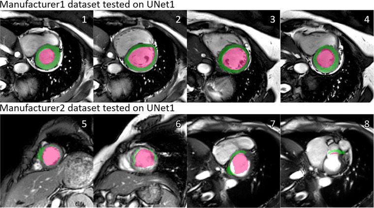
As an example, Figure 1 shows the segmentation results by U-Net 1 on the testing data from manufacturer 1 and manufacturer 2, respectively. A severe performance drop can be observed. In Table 2, we report the performance in terms of Dice index in all cross-manufacturer experiments. For all three manufacturer-specific U-Nets, segmentation performance was optimal on the testing datasets from the same manufacturer. When applied to data from a different manufacturer, the performance dropped significantly (P < .05 in all cases). As shown in Table 2, the reduction of performance, as quantified by the change of Dice index, was as high as 24%, 29%, and 33% for U-Net 1, U-Net 2, and U-Net 3, respectively.

Figure 1:

Illustration of the manufacturer shift problem. The upper row shows the performance of U-Net 1 tested on datasets from manufacturer 1, and the lower row shows the performance of U-Net 1 tested on datasets from manufacturer 2. A performance drop can be observed, in the form of undersegmentation. Numbers at upper right corner of each subfigure indicate different examples. Green regions denote the automatic myocardium segmentation results by the U-Net, while red regions denote the blood pool segmentation results.

Table 2:

Dice Indexes of Segmentation Network Trained and Tested on Different MRI Scanner Manufacturer Data

Manufacturer Adaptation

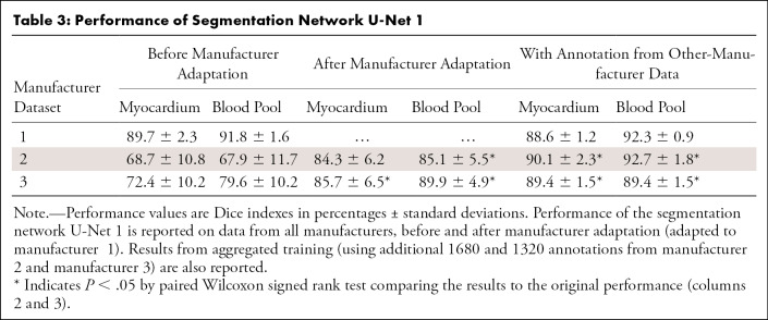
We evaluated the manufacturer adaptation performance also in terms of LV segmentation accuracy. Table 3 reports the Dice indexes before and after manufacturer adaptation. The reference performance of a CNN trained with enlarged annotation data was also reported. While this CNN trained on the most extensive dataset yielded the best performance overall, manufacturer adaptation significantly improved the cross-manufacturer performance without the need of extra annotation (up to 37% and 18% for manufacturer 2 and manufacturer 3, respectively). The performance of the reference methods is reported in Appendix E1 (supplement).

Table 3:

Performance of Segmentation Network U-Net 1

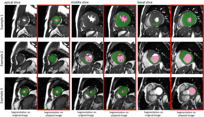
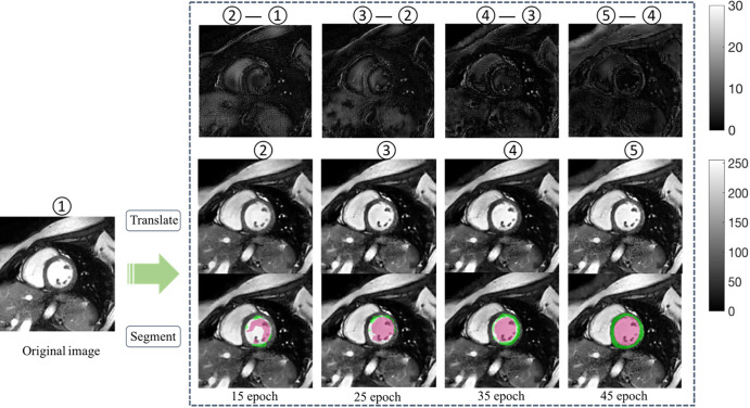
Figure 2 shows some typical examples of the segmentation results before and after manufacturer adaptation. It can be observed that manufacturer shift caused mostly undersegmentation; namely, part of the LV failed to be segmented. After manufacturer adaptation, the undersegmentation phenomenon was reduced. Figure 3 shows an example of the adapted image at the different stages of CycleGAN training. To better appreciate the changes, we calculated the difference images and zoomed in on the grayscale. The segmentation results for the adapted images at different stages are also shown in Figure 3. It can be observed that the segmentation results gradually improved when the CycleGAN progressively learned to generate images with similar characteristics to the training dataset.

Figure 2:

Three examples show boost of segmentation performance after manufacturer adaptation. Examples from apical, middle, and basal slices are given. In each subfigure, the left column shows segmentation results on original data from another manufacturer, while the right (red box) shows segmentation results on manufacturer-adapted data. Green regions denote the automatic myocardium segmentation results by the U-Net, while red regions denote the blood pool segmentation results.

Figure 3:

The performance of U-Net trained on one manufacturer dataset improved on dataset from another manufacturer, along with training epochs. Middle row shows adapted images at different epochs. Bottom row shows the corresponding segmentation results after manufacturer adaptation using the same U-Net. Upper row illustrates the subtle difference between the adapted images (scale indicated by gray-scale bar). Numbers 1–5 mark image at different adaptation stages, with 5 being the final adapted image. Green regions denote the automatic myocardium segmentation results by the U-Net, while red regions denote the blood pool segmentation results.

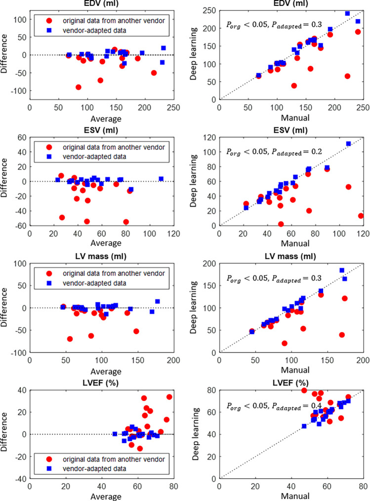
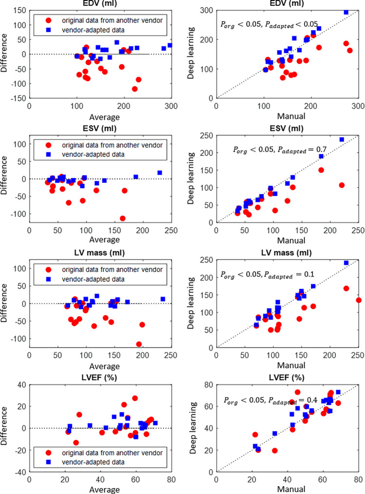
Clinical parameters, namely, EDV, ESV, LV mass, and LVEF, were computed from the automated segmentation results. Figure 4 and Figure 5 show the results before and after manufacturer adaptation for manufacturer 2 and manufacturer 3, respectively. The results were then compared with the parameters calculated from reference standard manual annotation. All clinical parameters, including EDV, ESV, LV mass, and LVEF, were significantly different from the ground truth when the U-Net trained on the manufacturer 1 dataset was directly applied to the manufacturer 2 and manufacturer 3 datasets (P < .05 by the paired Wilcoxon signed rank test). However, significant improvement can be observed after manufacturer adaptation. In particular, the undersegmentation phenomenon that typically occurred in cross-manufacturer segmentation was reduced. After manufacturer adaptation, most clinical parameters were not significantly different from the ground truth measurements, with the only exception being the EDV parameter for the manufacturer 3 dataset, with P < .05 (Figs 4, 5). For LVEF, manufacturer adaptation resulted in an improved Pearson correlation of 0.89 and 0.94 with the ground truth for the manufacturer 2 and manufacturer 3 datasets, respectively, compared with the correlation without manufacturer adaptation: 0.005 and 0.77, respectively. For the manufacturer 2 dataset, the LVEF derived from the original data had virtually no correlation with the true values, due to the seriously underestimated blood pool at the systolic phase, which is usually more difficult to segment than the diastolic phase due to blurring of blood-myocardium boundaries.

Figure 4:

Bland-Altman plots of quantitative parameters derived by automated segmentation for manufacturer 2 data, compared with the manual reference standard. Red dots represent results before manufacturer adaptation, and blue squares represent results after manufacturer adaptation. Four quantitative parameters are reported: end-systolic volume (ESV), end-diastolic volume (EDV), left ventricular (LV) mass, and left ventricular ejection fraction (LVEF). The P values by the paired Wilcoxon signed rank test were reported: P_org is P value comparing results from the original MRI with the ground truth, P_adapted is P value comparing results from the manufacturer-adapted MRI with the ground truth.

Figure 5:

Bland-Altman plots of quantitative parameters derived by automated segmentation for manufacturer 3 data, compared with the manual reference standard. Red dots represent results before manufacturer adaptation, blue squares represent results after manufacturer adaptation. Four quantitative parameters are reported: end-systolic volume (ESV), end-diastolic volume (EDV), left ventricular (LV) mass, and left ventricular ejection fraction (LVEF). The P values by the paired Wilcoxon signed rank test were reported: P_org is P value comparing results from the original MRI with the ground truth, P_adapted is P value comparing results from the manufacturer-adapted MRI with the ground truth.

Discussion

In this study, we highlighted the MRI manufacturer shift problem, a bottleneck to the widespread use of deep learning tools in practice. We showed that by adapting the MRI data statistically using the CycleGAN method, a deep learning segmentation tool can be better extended to multimanufacturer use without additional manual annotation.

In recent years, there has been a substantial increase in deep learning research for radiologic image analysis. Deep learning methods have reported expert-level performance on many organ-segmentation tasks (4,21,22). However, there is still limited research on the generalizability of these deep learning segmentation tools, especially in a clinical scenario where variability simply arises from different scanner manufacturers. In this study, we quantified how manufacturer shift could negatively affect the performance of a well-trained CNN segmentation tool. In practice, this implies that a model well trained and well validated on one dataset cannot be reliably extended to other-manufacturer data.

To address the manufacturer shift problem, we can increase the variability of the training data as in a recent multimanufacturer, multicenter study (4), which showed that the CNN model trained with datasets of higher heterogeneity could generalize better to new datasets. In our study, increasing the training image variability also significantly improved the generalization performance by retraining with additional annotated data from other manufacturers. The solution, however, is expensive in practice, requiring new annotations each time. Alternatively, one can also use transfer learning to utilize a previously trained CNN and fine-tune it with a limited set of annotated data (23,24). From a design point of view, we can certainly reduce the complexity of the deep learning models or add regulation terms to suppress the overfitting and improve the generalizability. Nevertheless, a balance between bias and variance always exists in the machine learning theory (9,25): A model may generalize better at the cost of reduced accuracy, which is undesirable in clinical use. Our study presented an alternative solution: Instead of pushing the limits on the training data or the CNN model, we preprocess the data by adapting it to the same underlying distribution as that of the training data, such that it better fits the training model. We observed a performance boost after manufacturer adaptation. We note that the manufacturer 1 (3.0 T) CNN (U-Net 1) generalized better to the manufacturer 3 (3.0 T) dataset than to the manufacturer 2 (1.5 T) dataset. This may reflect some inherent rules of manufacturer shift: The CNN can be sensitive to signal-to-noise ratio and frequency details that are related to field strength.

GAN is one of the most intriguing ideas in deep learning: to generate fake data by learning from real data (17). Since its introduction in 2014, GAN has inspired many new interesting research endeavors in computer vision. With GAN, exceedingly convincing fake images of animals, humans, and natural scenes can be generated through learning a large quantity of real images (26,27). For medical image applications, the use of GAN should however be cautioned against, as such “generation” can be detrimental to the radiologic practice. GAN can generate fake medical images that appear authentic but likely miss local details specific to a patient. Critical cases are examples of abnormally heterogeneous texture smoothed out or possible formation and deformation of local details (eg, nodules, tumor, or myocardial scar). Risk arises if these images are to be used for diagnosis or clinical decision making. In this work, however, we used GAN merely as a preprocessing step for segmentation. Cine images are not to visualize foci tissue fibrosis, instead they are acquired for measuring the overall cardiac structure and function. In this scenario, the concern is less the high-frequency image details, but the global image style in terms of illuminance, contrast, and edge sharpness, which CycleGAN is especially good at handling (14).

We observed that the difference between the original MR image and manufacturer-adapted image was very subtle. For radiologists, the two images make no difference for manual segmentation, but when fed to the trained deep learning segmentation tool, such a subtle change can lead to markedly different results. This is another proof that the deep learning tool may be vulnerable, and that it has not gained human-level cognition, as argued by the adversarial theory (17). Poor generalizability is one consequence of its vulnerability; further research is warranted to fundamentally improve its cognition level.

A limitation of this study was that the annotated data from three manufacturers were unbalanced in number. The patient demographics were also not matched. To avoid confounding the manufacturer adaptation performance with the segmentation network performance, we chose to only validate the manufacturer adaptation on the U-Net trained with the largest number of annotations.

In conclusion, we have quantitatively measured the performance drop caused by MRI manufacturer shift and proposed a solution: manufacturer adaptation based on GAN. Our work showed that manufacturer adaptation could largely increase the generalizability of an existing deep learning tool, extending its use to data from different manufacturers without new annotation. The improved generalization is essential for the widespread use of deep learning tools in clinical practice.

References

- 1.McRobbie DW, Moore EA, Graves MJ, Prince MR. MRI from Picture to Proton. Cambridge Core. 2006. http://cambridge.org/core/books/mri-from-picture-to-proton/3ADC814FF8FC6A78A54D37746F806D5A. Accessed October 10, 2019. [Google Scholar]
- 2.Shen D, Wu G, Suk HI. Deep Learning in Medical Image Analysis. Annu Rev Biomed Eng 2017;19(1):221–248. [DOI] [PMC free article] [PubMed] [Google Scholar]
- 3.Lakhani P, Prater AB, Hutson RK, et al. Machine Learning in Radiology: Applications Beyond Image Interpretation. J Am Coll Radiol 2018;15(2):350–359. [DOI] [PubMed] [Google Scholar]
- 4.Tao Q, Yan W, Wang Y, et al. Deep Learning-based Method for Fully Automatic Quantification of Left Ventricle Function from Cine MR Images: A Multivendor, Multicenter Study. Radiology 2019;290(1):81–88. [DOI] [PubMed] [Google Scholar]
- 5.Kurata Y, Nishio M, Kido A, et al. Automatic segmentation of the uterus on MRI using a convolutional neural network. Comput Biol Med 2019;114:103438. [DOI] [PubMed] [Google Scholar]
- 6.Chen L, Bentley P, Mori K, Misawa K, Fujiwara M, Rueckert D. DRINet for Medical Image Segmentation. IEEE Trans Med Imaging 2018;37(11):2453–2462. [DOI] [PubMed] [Google Scholar]
- 7.Ronneberger O, Fischer P, Brox T. U-Net: Convolutional Networks for Biomedical Image Segmentation. In: Navab N, Hornegger J, Wells W, Frangi A, eds. Medical Image Computing and Computer-Assisted Intervention – MICCAI 2015. MICCAI 2015. Lecture Notes in Computer Science, vol 9351. Cham, Switzerland: Springer, 2015; 234–241. [Google Scholar]
- 8.LeCun Y, Bengio Y, Hinton G. Deep learning. Nature 2015;521(7553):436–444. [DOI] [PubMed] [Google Scholar]
- 9.Goodfellow I, Bengio Y, Courville A. Deep Learning. Cambridge, Mass: MIT Press, 2016. [Google Scholar]
- 10.Pooley RA. AAPM/RSNA physics tutorial for residents: fundamental physics of MR imaging. RadioGraphics 2005;25(4):1087–1099. [DOI] [PubMed] [Google Scholar]
- 11.Yan W, Wang Y, Gu S, et al. The Domain Shift Problem of Medical Image Segmentation and Vendor-Adaptation by Unet-GAN. In: Shen D, Liu T, Peters TM, et al., eds. Medical Image Computing and Computer Assisted Intervention – MICCAI 2019. MICCAI 2019. Lecture Notes in Computer Science, vol 11765. Cham, Switzerland: Springer, 2019; 623–631. [Google Scholar]
- 12.Bluemke DA, Moy L, Bredella MA, et al. Assessing Radiology Research on Artificial Intelligence: A Brief Guide for Authors, Reviewers, and Readers-From the Radiology Editorial Board. Radiology 2020;294(3):487–489. [DOI] [PubMed] [Google Scholar]
- 13.Allen B Jr, Seltzer SE, Langlotz CP, et al. A Road Map for Translational Research on Artificial Intelligence in Medical Imaging: From the 2018 National Institutes of Health/RSNA/ACR/The Academy Workshop. J Am Coll Radiol 2019;16(9 Pt A):1179–1189. [DOI] [PubMed] [Google Scholar]
- 14.Colletti PM. Multicenter, Scan-Rescan, Human and Machine Learning CMR Study to Test Generalizability and Precision in Imaging Biomarker Analysis: A Solid Basis for Future Work. Circ Cardiovasc Imaging 2019;12(10):e009759. [DOI] [PubMed] [Google Scholar]
- 15.Bhuva AN, Bai W, Lau C, et al. A Multicenter, Scan-Rescan, Human and Machine Learning CMR Study to Test Generalizability and Precision in Imaging Biomarker Analysis. Circ Cardiovasc Imaging 2019;12(10):e009214. [DOI] [PubMed] [Google Scholar]
- 16.Crammer K, Kearns M, Wortman J. Learning from Multiple Sources. J Mach Learn Res 2008;9(Aug):1757–1774. http://www.jmlr.org/papers/v9/crammer08a.html. Accessed October 10, 2019. [Google Scholar]
- 17.Goodfellow I, Pouget-Abadie J, Mirza M, et al. Generative Adversarial Nets. In: Ghahramani Z, Welling M, Cortes C, Lawrence ND, Weinberger KQ, eds. Advances in Neural Information Processing Systems 27. Red Hook, NY: Curran Associates, 2014; 2672–2680. http://papers.nips.cc/paper/5423-generative-adversarial-nets.pdf. Accessed October 10, 2019. [Google Scholar]
- 18.Zhu JY, Park T, Isola P, Efros AA. Unpaired Image-to-Image Translation using Cycle-Consistent Adversarial Networks. arXiv:170310593 [cs] [preprint] http://arxiv.org/abs/1703.10593. Posted March 30, 2017. Accessed October 10, 2019.
- 19.Bai W, Sinclair M, Tarroni G, et al. Automated cardiovascular magnetic resonance image analysis with fully convolutional networks. J Cardiovasc Magn Reson 2018;20(1):65. [DOI] [PMC free article] [PubMed] [Google Scholar]
- 20.Zou KH, Warfield SK, Bharatha A, et al. Statistical validation of image segmentation quality based on a spatial overlap index. Acad Radiol 2004;11(2):178–189. [DOI] [PMC free article] [PubMed] [Google Scholar]
- 21.Bernard O, Lalande A, Zotti C, et al. Deep Learning Techniques for Automatic MRI Cardiac Multi-Structures Segmentation and Diagnosis: Is the Problem Solved? IEEE Trans Med Imaging 2018;37(11):2514–2525. [DOI] [PubMed] [Google Scholar]
- 22.Bakas S, Reyes M, Jakab A, et al. Identifying the Best Machine Learning Algorithms for Brain Tumor Segmentation, Progression Assessment, and Overall Survival Prediction in the BRATS Challenge. arXiv:181102629 [cs, stat] [preprint] http://arxiv.org/abs/1811.02629. Posted November 5, 2018. Accessed March 26, 2020. [Google Scholar]
- 23.Chen A, Zhou T, Icke I, et al. Transfer Learning for the Fully Automatic Segmentation of Left Ventricle Myocardium in Porcine Cardiac Cine MR Images. In: Pop M, Sermesant M, Jodoin PM, et al., eds. Statistical Atlases and Computational Models of the Heart. ACDC and MMWHS Challenges. STACOM 2017. Lecture Notes in Computer Science, vol 10663. Cham, Switzerland: Springer, 2018; 21–31. [Google Scholar]
- 24.Raghu M, Zhang C, Kleinberg J, Bengio S. Transfusion: Understanding Transfer Learning for Medical Imaging. arXiv:190207208 [cs, stat] [preprint] http://arxiv.org/abs/1902.07208. Posted February 14, 2019. Accessed October 10, 2019.
- 25.Duda RO, Hart PE, Stork DG. Pattern Classification. 2nd ed. New York, NY: Wiley-Interscience, 2000. [Google Scholar]
- 26.Karras T, Laine S, Aila T. A Style-Based Generator Architecture for Generative Adversarial Networks. arXiv:181204948 [cs, stat] [preprint] http://arxiv.org/abs/1812.04948. Posted December 12, 2018. Accessed October 23, 2019. [DOI] [PubMed]
- 27.Suwajanakorn S, Seitz SM, Kemelmacher-Shlizerman I. Synthesizing Obama: Learning Lip Sync from Audio. ACM Trans Graph 2017;36(4):95:1–95:13. [Google Scholar]
Associated Data
This section collects any data citations, data availability statements, or supplementary materials included in this article.