Designing and Analyzing Clinical Trials for Personalized Medicine via Bayesian Models

Abstract

Patients with different characteristics (e.g., biomarkers, risk factors) may have different responses to the same medicine. Personalized medicine clinical studies that are designed to identify patient subgroup treatment efficacies can benefit patients and save medical resources. However, subgroup treatment effect identification complicates the study design in consideration of desired operating characteristics.

We investigate three Bayesian adaptive models for subgroup treatment effect identification: pairwise independent, hierarchical, and cluster hierarchical achieved via Dirichlet Process (DP). The impact of interim analysis and longitudinal data modeling on the personalized medicine study design is also explored. Interim analysis is considered since they can accelerate personalized medicine studies in cases where early stopping rules for success or futility are met. We apply integrated two-component prediction method (ITP) for longitudinal data simulation, and simple linear regression for longitudinal data imputation to optimize the study design. The designs’ performance in terms of power for the subgroup treatment effects and overall treatment effect, sample size, and study duration are investigated via simulation.

We found the hierarchical model is an optimal approach to identifying subgroup treatment effects, and the cluster hierarchical model is an excellent alternative approach in cases where sufficient information is not available for specifying the priors. The interim analysis introduction to the study design lead to the trade-off between power and expected sample size via the adjustment of the early stopping criteria. The introduction of the longitudinal modeling slightly improves the power. These findings can be applied to future personalized medicine studies with discrete or time-to-event endpoints.

1. Introduction

Personalized medicine is defined as the tailoring of treatment to patients based on their characteristics, needs, and preferences during medical care ^[1]. Therefore, personalized medicine clinical trials are designed to test for a treatment effect in patient subgroups ^{[2, 3]}. In general, these subgroups are defined using “personalized” or patient-specific characteristics such as biomarkers, demographics, and disease sub-categories. Personalized randomized clinical trials (RCTs) can be categorized as prospective, prospective-concurrent, prospective-retrospective, or retrospective based on the availability of the data relative to the design of the study ^[4]. Personalized RCTs are sufficiently powered to test for a treatment effect while controlling both the overall Type I error and the subgroup false positive rates ^[2]. However, personalized RCTs that optimize time and resource use without sacrificing statistical rigor are both essential and unexplored.

Recently, researchers have proposed both frequentist and Bayesian approaches to identifying subgroup treatment effect. Lipkovich et al.^[5] developed a frequentist non-parametric recursive partitioning method for the analysis of subgroup treatment effects. Another non-parametric method, random forests of interaction trees (RFIT), was proposed by Su et al. ^[6] to estimate subgroup treatment effects. Additionally, Foster et al. ^[7] created the virtual twins method, and Altstein et al. ^[8] suggested a new computational method for parameter estimation of an accelerated failure time (AFT) model with subgroups identified by a latent variable. Alosh et al. also introduced the solutions to solve the issues of chance findings, low power of interaction statistical tests for the treatment-by-subgroup interaction, etc. when executing the subgroup analysis from frequentist perspective ^[2].

Compared to the frequentist approaches, Bayesian adaptive designs have potential benefits for prospective personalized RCTs since they naturally extend from simple ^[9] to more complex but efficient models ^[10], and facilitate decision making in advance via interim analysis ^{[11, 12]}. Bayesian adaptive designs also provide the probability that a treatment is best for a particular subgroup ^[13], which has a straightforward interpretation and thus is friendly to scientific researchers with little statistical background. Additionally, the Food and Drug Administration (FDA) recently released guidelines that encourage the use of prespecified interim analysis in personalized medicine adaptive designs to evaluate subgroup factors and modify the subpopulation enrollment accordingly ^[14]. Finally, Bayesian adaptive designs can illustrate the effectiveness of a treatment in subpopulations or the overall population with higher power when compared to a fixed design of the same size^[15] .

The focus of this research is a prospective study design where different subgroup treatment effects have already been noted but must be investigated in a confirmatory environment. A study design in terms of Bayesian models, longitudinal data, and interim analysis is involved ^{[2, 16, 17]}. Research has been done for trials whose purpose is to identify a single subgroup ^[18], which may be useful for seamless phase II to III designs ^{[19, 20]}. In addition, Hobbs et al. ^[21] have proposed an innovative sequential basket trial design formulated with Bayesian monitoring rules based on multisource exchangeability and hierarchical modeling.

Some studies ^[22–24] refer to RCTs for adaptive personalized medicine. Personalized medicine designs adjust enrollment of subjects for specific subgroups at interims to maximize power and/or shorten study duration ^[14]. It should be noted that our research does not adjust the randomization ratio after interim analysis. Additionally, this research is motivated by comparative effectiveness and thus aims to identify the best treatment by subgroup, avoiding the term “futility”, as one treatment’s futility is another’s success.

One of the trending issues in RCTs for personalized medicine is the handling of multiplicity across subgroups. A well-calibrated RCT will have a Type I error rate of 5% (based on two-sided test) or 2.5% (based on one-sided test), and this frequentist calibration is also crucial for Bayesian RCTs ^{[25, 26]}. Much effort in group sequential designs ^[27] is spent controlling the familywise Type I error rate because of the multiple points of testing due to both the number of subgroups and the number of interim analyses. Random effects linear models for identification of subgroup treatment effects with longitudinal data have also been presented ^[28], but little research exists on Bayesian models for longitudinal data with subgroup treatment effects identification. A more effective modeling approach is to borrow strength across the subgroups via a Bayesian hierarchical model. Berry et al. ^[15] concluded that this type of modeling provides a better chance at identifying efficacy or futility than the models that promote independence across subgroups. Gamalo-Siebers et al.^[29] pointed out that in some instances, hierarchical models suffer from “over-shrinkage” and a Dirichlet Process (DP) prior is a possible alternative to the lighter-tailed alternatives. Hierarchical models and DP priors are also candidate models in this research.

This research is the result of a National Center for Advancing Translational Sciences (NCATS) national working group with the name of Designing and Analyzing Clinical Trials for Personalized Medicine (DACTPerM), brought together to explore the properties of several statistical models to be applied to academic medical RCTs for personalized medicine. The exploration is done by simulating trials in which several treatments are tested simultaneously (e.g., two drugs tested in different sub-populations). Interim analyses are specified at a fixed number of subjects enrolled; stopping rules for success are based on posterior probability criteria set for individual subgroups. Longitudinal modelling imputation for missing data is also explored to improve the study design.

In Section 2, we introduce the motivating study, Patient Assisted Intervention for Neuropathy: Comparison of Treatment in Real Life Situations (PAIN-CONTRoLS) ^[30], and several models for RCTs in personalized medicine are described as well. In Section 3, operating characteristics for the different possible designs are presented and compared. We demonstrate the models’ simulation-based performance. We conclude with discussion and conclusions in Section 4.

2. Methods

2.1. Motivating Study

The objective of the PAIN-CONTRoLS study was to identify the most effective medicine for reducing pain and improving the quality of life in patients with Cryptogenic Sensory Polyneuropathy (CSPN). The study investigates four candidate medicines: nortriptyline, duloxetine, pregabalin, and mexiletine. The study found that both nortriptyline and duloxetine had the highest posterior probability of being the best treatment among the four candidates. However, an exploratory analysis found that nortriptyline and duloxetine had results that varied by subject characteristics such as gender, age, and race. Therefore, we wish to design a future prospective trial that verifies this subgroup hypothesis via an innovative and efficient Bayesian model. The primary endpoint, pain, is an approximately continuous measure of risk reduction in pain (scale 0-10) at 12-weeks relative to that at randomization. Specifically, it is equal to $\frac{P_0-P_{12}}{P_0}$, where P₀ is pain score at randomization and P₁₂ is the one at 12 weeks.

2.2. Model Specification

Selecting a model for personalized medicine RCTs is important for optimizing operating characteristics. Generally, it is unlikely that one model can be recommended for all RCTs. The strategy for model selection is to pick the candidate model with the most desirable operating characteristics estimated via simulation. It is also a good strategy to build the candidate models from simple to complex. A pairwise independent subgroup model (i.e., a model for one subgroup is independent of those for the other subgroups) is a straightforward one to begin with. We also consider the hierarchical and cluster hierarchical model since these models adapt depending on the variation of the treatment effect across subgroups.

Generally, we assume the endpoints for all subjects from both treatment arms (A or B), i.e., both Arm A and B are active arms which means our research is based on effectiveness comparison, are normally distributed with identical standard deviations but different means.

Specifically, observations from arm A are denoted:

$$Y_{1g}^{\left(A\right)},Y_{2g}^{\left(A\right)},Y_{3g}^{\left(A\right)},Y_{4g}^{\left(A\right)}\dots .Y_{N_g^{\left(A\right)}g}^{\left(A\right)}~N\left({\gamma }_g,{\sigma }^2\right);$$

and for arm B:

$$Y_{1g}^{\left(B\right)},Y_{2g}^{\left(B\right)},Y_{3g}^{\left(B\right)},Y_{4g}^{\left(B\right)}\dots .Y_{N_g^{\left(B\right)}g}^{\left(B\right)}~N\left({\gamma }_g+{\theta }_g,{\sigma }^2\right),$$

where g is the index indicating the subgroup and g ∈ {1, 2, 3,… g_n}. $N_g^{\left(A\right)}$ and $N_g^{\left(B\right)}$ represent the sample size of subgroup g for treatment arm A and B, respectively. The common standard deviation is given by σ and the means for arm A and B are γ_g and γ_g + θ_g, respectively. Thus, θ_g represents the treatment difference for subgroup g.

2.2.1. Pairwise Independent Model

In a pairwise independence model, separate priors are used for each treatment arm such that each γ_g and θ_g have normal prior distributions, ${\gamma }_g~N\left({\mu }_g^{\left(A\right)},{\tau }_g^{\left(A\right),2}\right)$, ${\theta }_g~N\left({\mu }_g^{\left(B\right)},{\tau }_g^{\left(B\right),2}\right)$, and ${\sigma }^2~IG\left(\frac{{\sigma }_n}{2},\frac{{\sigma }_{\mu }^2{\sigma }_n}{2}\right)$. We assume ${\tau }_g^{\left(A\right),2}$ is equal to ${\tau }_g^{\left(B\right),2}$, and ${\sigma }_{\mu }$ and ${\sigma }_n$ are the central and weight parameters of the inverse gamma distribution. We use weakly informative priors whose information was obtained from the example study and inflate the related prior variance values to diminish the effect that priors play in the following simulations. The complete conditional distributions of treatment difference $\left({\theta }_g\right)$ and treatment effect from arm $A\left({\gamma }_g\right)$, given data and all other parameters, are both normal. Specifically,

$${\theta }_g|Y_{1g}^{\left(B\right)}..Y_{N_g^{\left(B\right)}g}^{\left(B\right)},{\gamma }_g,{\sigma }^2,{\mu }_g^{\left(B\right)},{\tau }_g^{\left(B\right),2}~N\left(\frac{{\tau }_g^{\left(B\right),2}{N}_g^{\left(B\right)}\left({\overline{Y}}_g^{\left(B\right)}-{\gamma }_g\right)+{\sigma }^2{\mu }_g^{\left(B\right)}}{N_g^{\left(B\right)}{\tau }_g^{\left(B\right),2}+{\sigma }^2},\frac{{\tau }_g^{\left(B\right),2}{\sigma }^2}{N_g^{\left(B\right)}{\tau }_g^{\left(B\right),2}+{\sigma }^2}\right)$$ (1),

$${\gamma }_g|Y_{1g}^{\left(A\right)}\dots Y_{N_g^{\left(A\right)}g}^{\left(A\right)},Y_{1g}^{\left(B\right)}..Y_{N_g^{\left(B\right)}g}^{\left(B\right)},{\theta }_g,{\sigma }^2,{\mu }_g^{\left(A\right)},{\tau }_g^{\left(A\right),2}~N\left(\frac{{\tau }_g^{\left(A\right),2}\left(N_g^{\left(A\right)}{\overline{Y}}_g^{\left(A\right)}+N_g^{\left(B\right)}{\overline{Y}}_g^{\left(B\right)}-N_g^{\left(B\right)}{\theta }_g\right)+{\sigma }^2{\mu }_g^{\left(A\right)}}{\left(N_g^{\left(A\right)}+N_g^{\left(B\right)}\right){\tau }_g^{\left(A\right),2}+{\sigma }^2},\frac{{\tau }_g^{\left(A\right),2}{\sigma }^2}{\left(N_g^{\left(A\right)}+N_g^{\left(B\right)}\right){\tau }_g^{\left(A\right),2}+{\sigma }^2}\right)$$ (2).

2.2.2. Hierarchical Model

The hierarchical model’s borrowing strength across subgroups is achieved through shared prior distributions for each treatment. Consequently, ${\mu }_{\gamma }^{\left(A\right)}$, ${\mu }_{\gamma }^{\left(B\right)}$ and ${\tau }_{\gamma }^{\left(A\right),2}$, ${\tau }_{\gamma }^{\left(B\right),2}$ are considered random parameters from a set of shared distributions. For treatment arm A (γ_g):

$${\gamma }_g~N\left({\mu }_{\gamma }^{\left(A\right)},{\tau }_{\gamma }^{\left(A\right),2}\right),{\mu }_{\gamma }^{\left(A\right)}~N\left({\mu }_0,{\sigma }_2^0\right),{\tau }_{\gamma }^{\left(A\right),2}~IG\left(\frac{{\tau }_n}{2},\frac{{\tau }_{\mu }^2{\tau }_n}{2}\right);$$

and for the difference between treatment arms in subgroup g (θ_g):

$${\theta }_g~N\left({\mu }_{\gamma }^{\left(B\right)},{\tau }_{\gamma }^{\left(B\right),2}\right),{\mu }_{\gamma }^{\left(B\right)}~N\left({\mu }_0,{\sigma }_2^0\right),{\tau }_{\gamma }^{\left(B\right),2}~IG\left(\frac{{\tau }_n}{2},\frac{{\tau }_{\mu }^2{\tau }_n}{2}\right).$$

Here, ${\mu }_{\gamma }^{\left(A\right)}$ and ${\mu }_{\gamma }^{\left(B\right)}$ are independent and identically distributed, as are ${\tau }_{\gamma }^{\left(A\right),2}$ and ${\tau }_{\gamma }^{\left(B\right),2}$. We specify the values of the hyperparameters μ₀, ${\sigma }_0^2$, τ_n and ${\tau }_{\mu }^2$ when simulation is executed. The expressions of the completely conditional distributions of the treatment difference (θ_g) and the treatment effect from arm A (γ_g) given data and all other parameters are identical to (1) and (2) from the pairwise independent model. However, the complete conditional distributions of ${\mu }_{\gamma }^{\left(A\right)}$ and ${\mu }_{\gamma }^{\left(B\right)}$ given data and all other parameters are given by

$${\mu }_{\gamma }^{\left(B\right)}|{\theta }_1..{\theta }_{g_n},{\tau }_{\gamma }^{\left(B\right),2},{\mu }_0,{\sigma }_0^2~N\left(\frac{{\sigma }_0^2{\Sigma }_{g=1}^{g_n}{\theta }_g+{\tau }_{\gamma }^{\left(B\right),2}\mu {}_0}{g_n{\sigma }_0^2+{\tau }_{\gamma }^{\left(B\right),2}},\frac{{\tau }_{\gamma }^{\left(B\right),2}{\sigma }_0^2}{g_n{\sigma }_0^2+{\tau }_{\gamma }^{\left(B\right),2}}\right)$$ (3);

$${\mu }_{\gamma }^{\left(A\right)}|{\gamma }_1..{\gamma }_{g_n},{\tau }_{\gamma }^{\left(A\right),2},{\mu }_0,{\sigma }_0^2~N\left(\frac{{\sigma }_0^2{\Sigma }_{g=1}^{g_n}{\gamma }_g+{\tau }_{\gamma }^{\left(A\right),2}\mu {}_0}{g_n{\sigma }_0^2+{\tau }_{\gamma }^{\left(A\right),2}},\frac{{\tau }_{\gamma }^{\left(A\right),2}{\sigma }_0^2}{g_n{\sigma }_0^2+{\tau }_{\gamma }^{\left(A\right),2}}\right)$$ (4).

2.2.3. Cluster Hierarchical Model

The cluster hierarchical model is a non-parametric Bayesian method that uses a Dirichlet process with scale parameter, α and base distribution, G₀ ^[31]. Specifically, a random distribution, G, is drawn from the base distribution, G₀. The scale parameter α determines the discreteness of the random distribution G, and it varies from a single discrete point mass to the base distribution G₀ as α goes from zero to infinity. The random distribution G is considered a combination of clusters, and the data from one subgroup are drawn from some certain cluster. In the DACTPerM study, for subject i in subgroup g from cluster w_c, the subject’s response is given by

$$Y_{ig}|w_c~F\left(w_c\right)$$

$$w_c~G$$

$$G~DP\left(\alpha ,G_0\right);$$

where $G_0=N\left({\mu }_0,{\sigma }_0^2\right)$, and ${\mu }_0$ and ${\sigma }_0^2$ are identical to those from the hierarchical model presented previously. In addition, $F\left(w_c\right)=N=\left(({\mu }_{\gamma }^{\left(A\right)}+{\mu }_{\gamma }^{\left(B\right)})|{}_{w_c},{\tau }_{\gamma }^2|{}_{w_c}\right)$, and ${\mu }_{\gamma }^{\left(A\right)}$ and ${\mu }_{\gamma }^{\left(B\right)}$ have the same interpretation as those from the hierarchical model. Here, ${\tau }_{\gamma }^2$ is shared across arms A and B. Detailed specifications regarding the three models and derivations can be found in the appendix.

2.3. Study Design Considerations

The study design is assessed by the properties and performance of candidate models under varying assumptions and conditions prior to study execution. However, when simulating a clinical trial, apart from the analysis model and its parameters, a variety of functional factors must be considered to obtain reliable results. Those factors include, but are not limited to, the number of interim analyses, visit information, treatment allocation ratios, and accrual and drop-out rates. We define all the functional input as functional parameters, and those directly related to the response models, longitudinal modeling, and imputation as model parameters.

2.3.1. Design Inputs

Models for treatment.

As discussed in Section 2.2, three candidate models are considered for the statistical analysis plan and protocol: a pairwise independent model, a hierarchical model, and a cluster hierarchical model. All priors are specified based on the PAIN-CONTRoLS study.

Interim analysis and early evaluation criteria.

Interim analysis is important for the execution of an adaptive clinical trial, as it provides the means by which the design uses accumulating data to adapt. In this simulation, designs that include and exclude interim analysis are considered to assess their impact on operating characteristics. If interim analysis is included, all related early evaluation criteria are specified simultaneously for all subgroups. Specifically, the early success definition is that the posterior probability of one arm better than the other one is greater than the criterion (i.e. threshold) since both arms are active. I.e., the early success definition is that P(θ_g > 0 | Data) > criterion for all g, which indicates Arm B is successful; or, P(θ_g < 0 | Data) > criterion for all g, which indicates Arm A is successful. This study will stop for early success when it meets the early success definition.

Final evaluation criteria.

The final success criteria, like the early success criteria, are a function of the posterior probability one treatment arm being better than the other. Moreover, the final evaluation threshold values differ since we would like to control the overall type I error equal to 5%. Specifically, the final success definition is that the posterior probability of one arm better than the other one is greater than the threshold for some subgroup. I.e., the final success definition is that P(θ_g > 0 | Data) > criterion for some g, which indicates Arm B is successful; or, P(θ_g < 0 | Data) > criterion for some g, which indicates Arm A is successful.

To sum up, if no interim analysis is involved in the study design, the final success definition is that P(θ_g > 0 | Data) > criterion for some g; or, P(θ_g < 0 | Data) > criterion for some g. The type I error is controlled via the formula (5) below:

$$\mathrm{Pr}\left[P\left({\theta }_g>0|Data\right)>C_f\text{for some}g|H_0\right]+\mathrm{Pr}\left[P\left({\theta }_g<0|Data\right)>C_f\text{for some}g|H_0\right],$$ (5)

where H₀ corresponds to no effect scenario (introduced in Section 2.3.3), and it means there is no treatment differences between Arm A and B for all subgroups. C_f means the criterion used for final analysis and it is adjusted to meet the type I error equal to 0.05 for each study design. The power is obtained via the formula (6) below:

$$Pr\left[P\left({\theta }_g>0|Data\right)>C_f\text{for some}g|H_1\right]+Pr\left[P\left({\theta }_g<0|Data\right)>C_f\text{for some}g|H_1\right],$$ (6)

where H₁ is correspondent to alternative scenarios (introduced in Section 2.3.3), and it means there is treatment differences between Arm A and B for some/all subgroups. Given one study design, the thresholds for alternative scenarios are identical to those from no effect scenario.

If interim analysis is involved in the study design, the early success definition is P(θ_g > 0 | Data) > criterion for all g; or, P(θ_g < 0 | Data) > criterion for all g. The final success definition is P(θ_g > 0 | Data) > criterion for some g; or, P(θ_g < 0 | Data) > criterion for some g. The type I error is controlled via the formula (7) below:

$$\mathrm{Pr}\left[P\left({\theta }_g>0|Data\right)>C_i\text{for all}g|H_0\right]+\mathrm{Pr}\left[P\left({\theta }_g<0|Data\right)>C_i\text{for all}g|H_0\right]+\mathrm{Pr}\left[P\left({\theta }_g>0|Data\right)>C_f\text{for some}g|H_0\right]+\mathrm{Pr}\left[P\left({\theta }_g<0|Data\right)>C_f\text{for some}g|H_0\right]$$ (7)

The power is obtained via the formula (8) below:

$$\mathrm{Pr}\left[P\left({\theta }_g>0|Data\right)>C_i\text{for all}g|H_1\right]+\mathrm{Pr}\left[P\left({\theta }_g<0|Data\right)>C_i\text{for all}g|H_1\right]+\mathrm{Pr}\left[P\left({\theta }_g>0|Data\right)>C_f\text{for some}g|H_1\right]+\mathrm{Pr}\left[P\left({\theta }_g<0|Data\right)>C_f\text{for some}g|H_1\right]$$ (8)

Where C_i means the criterion used for interim analysis, and the meanings of H₀ and H₁ are identical to those introduced under the study designs without interim analysis involved.

Given a specific study design involved in interim analysis, the thresholds of interim and final analyses are different, and they are adjusted to achieve the desired proportions of type I error spending on interim and final analyses. At an interim analysis the trial is a success and stops if all groups are successful, and at the final analysis the trial is a success if any groups are successful. The enrollment for a subgroup will stop at the interim if it meets the interim success criterion. Moreover, this subgroup will continue to follow up and re-analyze at final analysis based on the final success criterion. Moreover, we would like to control type I error less than 0.005 spending on interim analysis. These strategies will result in a longer study and provide more information for the researcher to draw the conclusion. The specific criteria value for interim and final analyses are provided in section 2.3.3 (Table 5). Once the thresholds of interim and final analyses are identified under the no effect scenario, they will be identically applied to the alternative scenarios.

Table 5.

Early and Final Evaluation Criteria.

Subgroup Number	Study design factor			Early evaluation criteria*		Final evaluation criteria&
	Model	Interim analysis involvement	longitudinal modelling involvement	Posterior probability for each subgroup	Boolean logic	Posterior probability for each subgroup	Boolean logic
4	Pairwise independent	No	No	----	----	0.9916	OR
4	Hierarchical	No	No	----	----	0.9805	OR
4	Cluster hierarchical	No	No	----	----	0.9822	OR
4	Pairwise independent	No	Yes	----	----	0.991	OR
4	Hierarchical	No	Yes	----	----	0.9777	OR
4	Cluster hierarchical	No	Yes	----	----	0.98	OR
4	Pairwise independent	Yes	No	0.9	AND	0.9932	OR
4	Hierarchical	Yes	No	0.9	AND	0.9818	OR
4	Cluster hierarchical	Yes	No	0.9	AND	0.9822	OR
4	Pairwise independent	Yes	Yes	0.9	AND	0.992	OR
4	Hierarchical	Yes	Yes	0.9	AND	0.979	OR
4	Cluster hierarchical	Yes	Yes	0.9	AND	0.9818	OR
8	Pairwise independent	No	No	----	----	0.9963	OR
8	Hierarchical	No	No	----	----	0.983	OR
8	Cluster hierarchical	No	No	----	----	0.9869	OR
8	Pairwise independent	No	Yes	----	----	0.9955	OR
8	Hierarchical	No	Yes	----	----	0.9818	OR
8	Cluster hierarchical	No	Yes	----	----	0.9865	OR
8	Pairwise independent	Yes	No	0.9	AND	0.9963	OR
8	Hierarchical	Yes	No	0.9	AND	0.9818	OR
8	Cluster hierarchical	Yes	No	0.9	AND	0.9851	OR
8	Pairwise independent	Yes	Yes	0.9	AND	0.9955	OR
8	Hierarchical	Yes	Yes	0.9	AND	0.981	OR
8	Cluster hierarchical	Yes	Yes	0.9	AND	0.985	OR

^*:The study will be identified as early success if all the subgroups meet the criteria. i.e. the posterior probability of (Arm B > Arm A, or Arm A > Arm B) for each subgroup meets the related criteria list the table above.

^&:The study will be identified as final success if any of the subgroups meet the criterion. i.e. the posterior probability of (Arm B > Arm A, or Arm A > Arm B) for any of the subgroups meet the related criterion list the table above.

Rates of accrual and drop out.

The accrual rate is an essential characteristic of a clinical trial since it determines trial duration. In adaptive designs, the accrual rate is even more important because the length of time between subject accrual and ascertainment of response determines the role of longitudinal data modeling in optimizing outputs. The accrual rate, together with drop-out rates, determine how many subjects are retained in the study. These rates for the simulation are based on the PAIN-CONTRoLS study.

Virtual endpoints.

The null scenario (no effect) is used to calibrate the study design to a Type I error rate of approximately 5%. This is done via an iterative process that updates early and final evaluation criteria until the Type I error rate approaches but does not exceed 5%. Several alternative hypotheses scenarios that use the same design parameters but have different response values are investigated.

Integrated two component prediction (ITP) is used for virtual endpoint simulation when longitudinal modeling is incorporated into the design. ITP allows endpoints to follow an exponential model over time with a subject-specific random effect to scale the visit values to the visit-specific specification of subgroup responses. Additionally, ITP does not affect the distribution of the final endpoint ^[28,32]. Three elements—the mean final endpoint, the of inter-subject ‘noise,’ and the noise at the current visit—along with the exponential function’s visit time and shape parameters determine the longitudinal data simulation at each visit ^[28]. A complete specification of the ITP model is in Appendix B.

Imputation via longitudinal modeling.

Longitudinal modeling is also applied for data imputation, and it is useful whether the trial is fixed or adaptive. Longitudinal modeling can be used in a fixed trial to impute endpoint values for patients that have dropped out of the study. In an adaptive design, it can be used for imputing endpoints values that have not yet been observed at an interim analysis, allowing the study to maximize the use of data to more efficiently adapt.

Simple linear regression (SLR) for Bayesian multiple imputation is used to model the relationship between responses observed at each pre-final visit and the unobserved (future) final visit. Specifically, for the future final response of subject i in subgroup g and treatment arm j,

$$Y_{i,g}^{\left(j\right)}|y_{it,g}^{\left(j\right)}~N\left({\alpha }_t+{\beta }_t{y}_{it,g}^{\left(j\right)},{\lambda }_t^2\right),$$

$${\alpha }_t~N\left({\alpha }_{\mu },{\alpha }_{\sigma }^2\right),{\beta }_t~N\left({\beta }_{\mu },{\beta }_{\sigma }^2\right),{\lambda }_t^2~IG\left(\frac{{\lambda }_n}{2},\frac{{\lambda }_{\mu }^2{\lambda }_n}{2}\right)$$

Where α_t and β_t are the intercept and slope at visit time t, and $y_{it,g}^{\left(j\right)}$ is the observed response for the subject i at visit time t. The model priors are specified identically across all visits (see Section 2.3.3).

The subjects’ pending and missing endpoints at interim analysis or missing ones at final analysis are imputed by the predicted distribution generated from multiple imputation via the SLR model. The imputed value from the predicted distribution captures both the uncertainty in the estimate of the parameters of the SLR model and the uncertainty of the prediction of the endpoint given particular parameter values ^[28].

Allocation.

Unequal allocation may be applied in some studies where sample size or randomization ratio adjustments are performed. Here, a 1:1 randomization ratio of subjects to the two treatment arms is fixed within each subgroup.

2.3.2. Design Outputs

Subgroup power.

Power can also be estimated in Bayesian studies via simulation. Subgroup power is defined as the probability that a subgroup meets the success criteria under the assumption that the subgroup responses from the two treatment arms are different.

Overall power (study success).

Simulations track the proportion of studies that show early success and final success based on the evaluation criteria (See Section 2.3.3). Overall power is estimated via the summation of both proportions, i.e., early and late success proportions. Both subgroup and overall power provide important model performance information and thus make the model assessment comprehensive.

Sample size.

Sample size is another key characteristic since it directly relates to the cost of running a trial. Thus, a study design that results in a lower sample size but similar power to a competing design is desirable. Compared to a fixed trial, an adaptive design can result in smaller sample sizes due to early stopping criteria.

Trial duration.

The trial duration is highly dependent upon accrual and sample size goals. It serves as a complimentary operating characteristic that the sponsor may consider when calculating trial cost prior to study execution.

2.3.3. Simulation Description

The simulation is executed for each study design in terms of an analysis model, interim analysis, and longitudinal modeling. Three analysis models are considered: pairwise independent, hierarchical, and cluster hierarchical. For each model, interim analysis and longitudinal modeling are either included or not. As Table 1 below indicates, the simulation is composed of three factors; there are twelve different study designs for the simulations.

Table 1.

Levels of the three factors for study design

Factor 1: Model	Factor 2: interim analysis involvement	Factor 3: Longitudinal modeling involvement
Pairwise independent Hierarchical Cluster hierarchical	Yes No	Yes No

To assess the designs comprehensively, we propose several alternative hypothesis scenarios that mimic the most frequent responses that can occur in real cases, and each scenario assumes a different response profile under two treatment arms. The specific scenarios include moderate and homogeneous effect, small and homogeneous effect, spread, opposite, and one nugget. Moreover, Arm B is assumed to have the effect for all the scenarios for the convenience of related formula and distribution specification. Supposing Arm A has the effect, the design outputs will be symmetric, as the related ones in which Arm B has the effect. Tables 2 and 3 present the specific virtual scenarios for four or eight patient subgroups. We assume the virtual response, a continuous measure of pain reduction, is normally distributed, in which higher values indicate better response to treatment. A common standard deviation (0.3) is specified for each subgroup of the two arms across all the scenarios, and this value is derived from the motivating example.

Table 2.

Four subgroup virtual response under six virtual treatment effect scenarios

Scenario*	Treatment	Subgroup 1	Subgroup 2	Subgroup 3	Subgroup 4
No effect	A	0	0	0	0
	B	0	0	0	0
Moderate and homogeneous effect	A	0	0	0	0
	B	0.17	0.17	0.17	0.17
Small and homogeneous effect	A	0	0	0	0
	B	0.085	0.085	0.085	0.085
Spread	A	0	0	0	0
	B	0.05	0.1	0.2	0.25
Opposite	A	0.17	0.17	0	0
	B	0	0	0.17	0.17
One nugget	A	0	0	0	0
	B	0	0.17	0	0

^*:The standard deviation of each subgroup virtual response for each scenario is 0.3.

Table 3.

Eight subgroup virtual responses under virtual treatment effect scenarios

Scenario*	Treatment	Subgroup 1	Subgroup 2	Subgroup 3	Subgroup 4	Subgroup 5	Subgroup 6	Subgroup 7	Subgroup 8
No effect	A	0	0	0	0	0	0	0	0
	B	0	0	0	0	0	0	0	0
Moderate and homogeneous effect	A	0	0	0	0	0	0	0	0
	B	0.17	0.17	0.17	0.17	0.17	0.17	0.17	0.17
Small and homogeneous effect	A	0	0	0	0	0	0	0	0
	B	0.085	0.085	0.085	0.085	0.085	0.085	0.085	0.085
Spread	A	0	0	0	0	0	0	0	0
	B	0.05	0.075	0.1	0.125	0.15	0.175	0.2	0.225
Opposite	A	0.17	0.17	0	0	0.17	0.17	0	0
	B	0	0	0.17	0.17	0	0	0.17	0.17
One nugget	A	0	0	0	0	0	0	0	0
	B	0	0.17	0	0	0	0	0	0

^*: The standard deviation of each subgroup virtual response for each scenario is 0.3.

Weakly informative priors that reflect the PAIN-CONTRoLS study are applied. In the cluster hierarchical model, a larger DP scale parameter will result in the random distribution being close to the base distribution, whereas a smaller DP scale parameter will result in a more discrete (point mass) random distribution. To differentiate it from the hierarchical model, the DP scale parameter is set to 2. All subgroups are assumed to have identical priors for the coefficient and intercept of SLR within each treatment arm. Though the prior mean values of the coefficient and intercept were obtained from PAIN-CONTRoLS, the prior standard deviation values of the coefficient and intercept were increased to 0.4 and 0.1 from 0.04 and 0.01, respectively, to reduce the impact of the motivating study data on simulation results. Table 4 presents the specific values for all priors involved in the simulation.

Table 4.

Prior specification for analysis models, longitudinal data imputation and longitudinal data simulation

Model	Parameter	Value
Pairwise independent*	prior mean of treatment arm A response for each subgroup (${\mathrm{\mu }}_{\mathrm{g}}^{\left(\mathrm{A}\right)}$)	0
	prior standard deviation of treatment arm A response for each subgroup (${\mathrm{\tau }}_{\mathrm{g}}^{\left(\mathrm{A}\right)}$)	0.3
	prior mean of treatment arm B response for each subgroup (${\mathrm{\mu }}_{\mathrm{g}}^{\left(\mathrm{B}\right)}$)	0
	prior standard deviation of treatment arm B response for each subgroup (${\mathrm{\tau }}_{\mathrm{g}}^{\left(\mathrm{B}\right)}$)	0.3
Hierarchical	hyperprior mean of all response prior mean (μ0)	0
	hyperprior standard deviation of all response prior mean (σ0)	0.1
	central parameter of inverse gamma distribution as which all response prior variance is distributed (τμ)	0.1
	weight parameter of inverse gamma distribution as which all response prior variance is distributed (τn)	2
Cluster hierarchical&	DP scale (α)	2
SLR @ - imputation for longitudinal data	prior mean of coefficient (βμ)	0.8
	prior standard deviation of coefficient (βσ)	0.4
	prior mean of intercept (αμ)	0
	prior standard deviation of intercept (ασ)	0.1
	central parameter of inverse gamma distribution as which imputed response variance is distributed (λμ)	0.18
	weight parameter of inverse gamma distribution as which imputed response variance is distributed (λn)	200/400
ITP $ - simulation for longitudinal data	fraction of the final treatment arm A response variance for each subgroup (${\mathrm{\omega }}_{\mathrm{g}}^{\left(\mathrm{A}\right)}$)	0.8
	fraction of the final treatment arm B response variance for each subgroup (${\mathrm{\omega }}_{\mathrm{g}}^{\left(B\right)}$)	0.8
	shape parameter of the exponential component for treatment arm A of each subgroup (${\mathrm{k}}_{\mathrm{g}}^{\left(\mathrm{A}\right)}$)	−10
	shape parameter of the exponential component for treatment arm B of each subgroup (${\mathrm{k}}_{\mathrm{g}}^{\left(\mathrm{B}\right)}$)	−10
Public parameter	central parameter of inverse gamma distribution as which all response variance is distributed (σμ)	1
	weight parameter of inverse gamma distribution as which all response variance is distributed (σn)	1

^*:We assume all subgroups from both treatment arms have identical prior means and standard derivation.

^&:Cluster hierarchical model maintains all hyperpriors from the hierarchical model and has additional DP scale parameter.

^@:All subgroups from both treatment arms are assumed to have same priors for the coefficient and intercept of SLR except for λ_n, and λ_n is specified as 200 for four subgroups and 400 for eight subgroups.

^$:Both fraction and shape parameter are specified identically within each subgroup from both treatment arms.

Early and final success criteria are designed to identify subgroup effects and study success. Study success at an interim analysis is defined to require success in all subgroups, but study success at study completion just requires success in any subgroup (specific criteria stated in Section 2.3.1). This results in a longer study and more conservative analysis. The concrete values for the early and final evaluation criteria are shown in Table 5. Operating characteristics such as power, sample size, and study duration under other effective virtual treatment scenarios with identical evaluation criteria from related no effect scenario are obtained accordingly via the simulations.

Table 6 presents the functional parameter values for the simulation, which are derived from PAIN-CONTRoLS. Subgroup sample sizes are set to 100, and the final sample size is determined via simulation with the consideration of Type I error and power. Study duration is specified as 12 weeks, and interim analysis will be executed once half the total number of subjects are enrolled. The study assumes three visits, with a 4-week lapse between consecutive visits. Each study design is simulated 10000 times.

Table 6.

Values of input functional parameters for study design

Functional factor	Value
Sample size per subgroup	100
Study duration	12 Weeks
Interim analysis execution time*	200 and 400 subjects enrolled for 4 and 8 subgroups
Visit times and duration between two consecutive visits*	3 visits; 4 weeks between visits
Allocation ratio of two arms within each subgroup	1:1
Accrual rate	4 /week
Drop-out rate	10 %

^*:Interim analysis execution time, specific visit times and duration between two consecutive visits are only involved when the study designs are with interim analysis and/or longitudinal data modeling.

3. Results

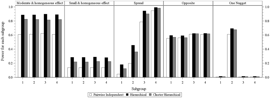
Subgroup power.

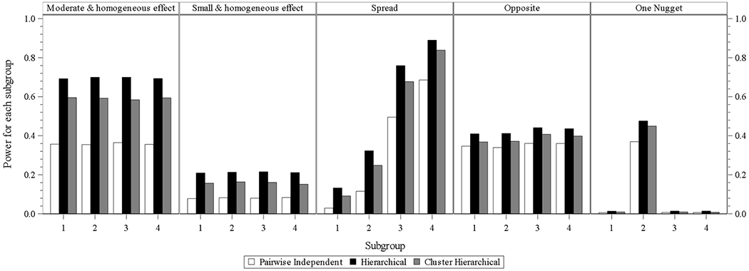
For the designs with four subgroups without interim analysis or longitudinal modeling (Fig. 1.1), the hierarchical model performs best in all the scenarios. The cluster hierarchical model performs similarly with mildly less power compared to the hierarchical model in the scenarios of opposite and one nugget. Similar findings can be identified from Fig. 1.2 which presents the designs with four subgroups without interim analysis and with longitudinal modeling. Each of the three models is with mildly higher power compared to that in each scenario under the design without interim analysis and without longitudinal modeling.

Fig. 1.1.

four subgroups power for design choice – model without interim analysis and without longitudinal modelling imputation

Fig. 1.2.

four subgroups power for design choice – model without interim analysis and with longitudinal modelling imputation

From Fig.1.3, which presents the subgroup power at the designs of three models with interim analysis and without longitudinal modeling, it can be observed that the three models’ performance order is identical to that from Fig.1.1. Each model is with a little less power compared to that in each scenario in Fig. 1.1.

Fig. 1.3.

four subgroups power for design choice – model with interim analysis and without longitudinal modelling imputation

In the designs of three models with interim analysis and with longitudinal modeling, the hierarchical model still performs best in all scenarios, and the performances of cluster hierarchical and pairwise independent model come to the second and third place. The power differences from hierarchical and cluster hierarchical models in one nugget scenario is larger than those from Fig. 1.1 to 1.3.

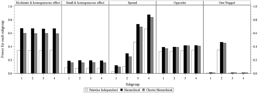
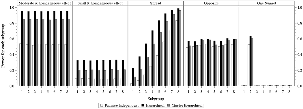
When subgroup number increases to 8, the subgroup power of the hierarchical model is still the highest within each subgroup of each scenario under the batch designs with identical involvement of interim analysis and longitudinal modeling. The power of the cluster hierarchical model for all subgroups within each subgroup under each design batch is lower than that from the hierarchical model but higher than that from a pairwise independent model.

Overall power (Study success).

It is easy to directly obtain the study power for each of the scenarios since it is equal to the final success proportion output from the simulation except for the opposite case. In the opposite scenario for four and eight subgroups, the overall power is estimated by the summation of proportion of simulated studies with any of subgroups in which the posterior probability of response from one arm higher than the response from other one satisfying the success criteria. The logic for this calculation is that there exists two treatment comparators and the study is successful if either arm within any subgroup meets the criteria. The overall power for the one nugget is consistent to the power from subgroup 2 in Fig. 1.1 to 2.4 presenting the subgroup power of related designs under different scenarios for both four and eight subgroups.

Fig. 2.4.

eight subgroups power for design choice – model with interim analysis and with longitudinal modelling imputation

In the designs of three models without interim analysis and longitudinal modeling, overall power is high and quite similar to the three models under the scenarios of the moderate and homogeneous effect and spread. Under the opposite scenario, the power of the hierarchical model is still high, and the power goes down slightly but is still high for the cluster hierarchical and pairwise independent models. The power of the hierarchical model under the all scenarios of the small and homogeneous effect, and one nugget is the highest. The power of the cluster hierarchical model under the same two scenarios decreases slightly, and the power of the pairwise independent model under the two scenarios is lower and with relatively larger differences compared to that from the hierarchical model. Similar findings are identified for the designs of three models without interim analysis and with longitudinal modeling. Each of the three models is with mildly higher power compared to that in each scenario under the design without interim analysis and without longitudinal modeling.

In the designs of three models with interim analysis and without longitudinal modeling, hierarchical and cluster hierarchical models perform similarly and have higher power than that for a pairwise independent model under each scenario.

In the designs of the three models with interim analysis and with longitudinal modeling, the hierarchical model has the highest power compared to the other two models in each scenario, and cluster hierarchical model performs closely to the hierarchical model with mildly decreased power. Performance of the pairwise independent model, same as that from the other design batch, is with the lowest power in each scenario. The same or quite similar comparison results are observed from eight subgroups.

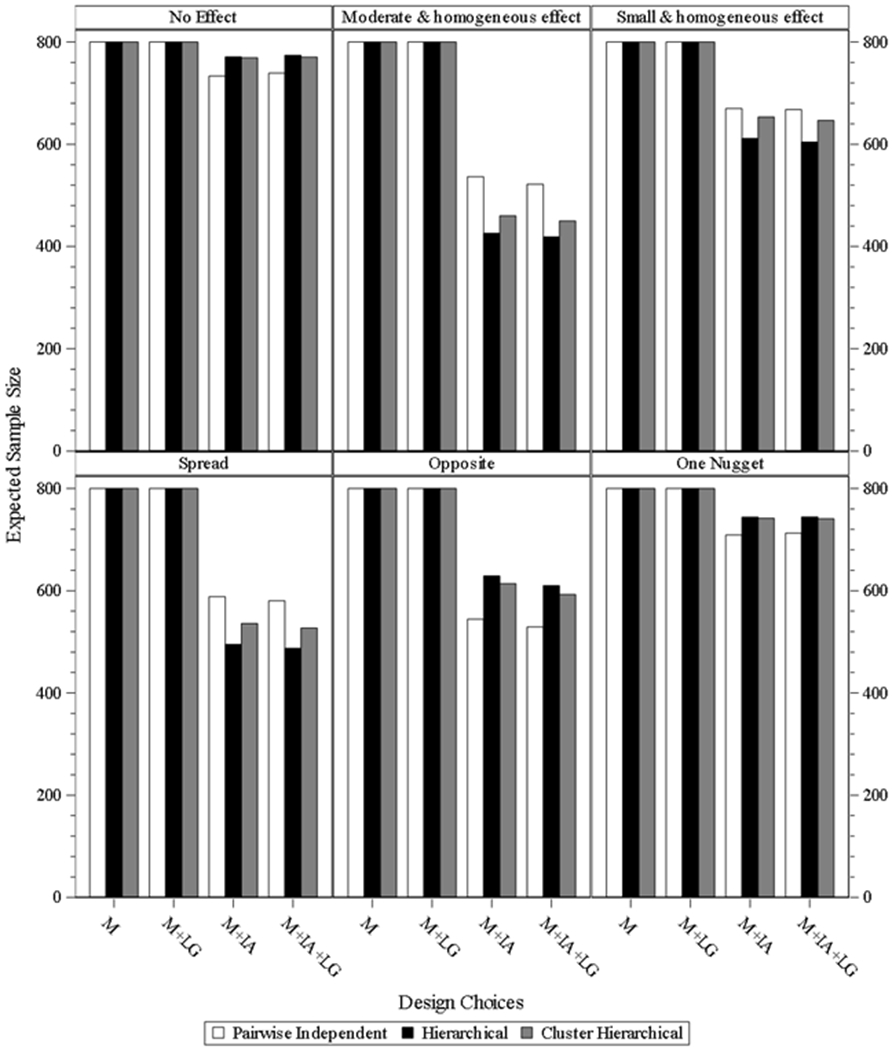
Sample size.

Fig. 4.1 & 4.2 present the expected sample size of designs under different scenarios for both four and eight subgroups. For the design batches of three models without interim analysis and with/without longitudinal modeling, the sample size is fixed as 100 subjects per subgroup. For the designs of the three models with interim analysis and without longitudinal modeling under the moderate and homogeneous effect and spread scenarios, the expected sample size dropped by 156 and 126 for hierarchical model, and by 141 and 115 for cluster hierarchical model, and by 119 and 104 for pairwise independent model. For the designs of the three models with interim analysis and with longitudinal modeling under the moderate and homogeneous effect and spread scenarios, the expected sample size approximately dropped by 167 and 134 for hierarchical model, and by 154 and 124 for cluster hierarchical model, and by 134 and 113 for pairwise independent model. The same trend is also observed under the small and homogeneous effect scenario, but all three models have higher expected sample size compared to the relevant one from the moderate and homogeneous effect and spread scenarios. However, under the scenarios of opposite and one nugget, pairwise independent is the best, and the other two models have higher expected sample size and perform similarly. The average expected sample sizes are approximately 330 and 360 for the two scenarios under the designs of the two models with interim analysis and without longitudinal modeling. The average expected sample sizes are approximately 310 and 360 for the two scenarios under the designs of the two models with interim analysis and with longitudinal modeling. Similar trends and comparison results are observed for eight subgroups.

Fig. 4.1.

expected sample size for study design under four subgroups. M = model without interim analysis and without longitudinal modelling imputation, M + LG = model without interim analysis and with longitudinal modelling imputation, M + IA = model with interim analysis and without longitudinal modelling imputation, M + IA + LG = model with interim analysis and with longitudinal modelling imputation.

Fig. 4.2.

expected sample size for study design under eight subgroups. M = model without interim analysis and without longitudinal modelling imputation, M + LG = model without interim analysis and with longitudinal modelling imputation, M + IA = model with interim analysis and without longitudinal modelling imputation, M + IA + LG = model with interim analysis and with longitudinal modelling imputation.

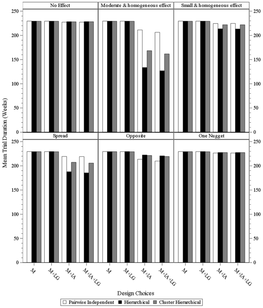
Trial duration.

Fig. 5.1 & 5.2 present the mean trial duration of the study designs under different scenarios for both four and eight subgroups. The same or similar findings of three models under different scenarios for both four and eight subgroups, as those from sample size observed since the trial duration is highly correlated to the sample size.

Fig. 5.1.

mean study duration for study desgin under four subgroups. M = model without interim analysis and without longitudinal modelling imputation, M + LG = model without interim analysis and with longitudinal modelling imputation, M + IA = model with interim analysis and without longitudinal modelling imputation, M + IA + LG = model with interim analysis and with longitudinal modelling imputation.

Fig. 5.2.

mean study duration for study desgin under eight subgroups. M = model without interim analysis and without longitudinal modelling imputation, M + LG = model without interim analysis and with longitudinal modelling imputation, M + IA = model with interim analysis and without longitudinal modelling imputation, M + IA + LG = model with interim analysis and with longitudinal modelling imputation.

Overall power comparison between hierarchical model and two independent sample t-test.

We also explored the overall power (study success) comparison between the hierarchical model and an approach that ignores the different subgroup effects and uses a classical-frequentist method—t-test without the involvement of interim analysis and longitudinal data. Table 7 below presents the concrete values from the two approaches. The powers of the Bayesian hierarchical model are much higher for the opposite and one nugget scenarios. This is because the subgroup treatment effects for these two scenarios are a challenge to identify at the study level for frequentist approach.

Table 7.

the overall power comparison between frequentist and our study.

Scenario	Treatment	Four subgroups				Eight subgroups
		Overall Effect	N Per Arm	Frequentist Power@	Our study Power *	Overall Effect	N Per Arm	Frequentist Power@	Our study Power *
No effect	A	0	200	0.05	0.05	0	400	0.05	0.05
	B	0	200			0	400
Moderate and homogeneous effect	A	0	200	0.99	0.997	0	400	0.99	1
	B	0.17	200			0.17	400
Small and homogeneous effect	A	0	200	0.81	0.6043	0	400	0.98	0.8417
	B	0.085	200			0.085	400
Spread	A	0	200	0.99	0.9984	0	400	0.99	0.9997
	B	0.15	200			0.1375	400
Opposite	A	0.085	200	0.05	0.9757	0.085	400	0.05	0.9987
	B	0.085	200			0.085	400
One nugget	A	0	200	0.29	0.6456	0	400	0.17	0.591
	B	0.0425	200			0.0213	400

^@:Power is calculated via the t-test for two independent sample to identify the treatment difference between the two arms.

^*:All the powers for each scenario are from the design of hierarchical model without interim analysis and without longitudinal data under four or eight subgroups, and the power is defined to identify the treatment difference between the two arms within subgroups.

4. Discussion and Conclusion

This paper explores the performance of three Bayesian models—pairwise independent, hierarchical, and cluster hierarchical—under different virtual responses for subgroups, including versions with interim analysis and longitudinal modeling. For all scenarios under each design, the hierarchical model generally performs better than the other two. This is because the hierarchical model is able to analyze the data using a mixture model, flexibly borrowing information from all subgroups and shrinking the subgroup means towards the central one, according to how similar they appear. The final output is sensitive to prior distribution specification and related prior value setting, and thus the hyperprior setting is an essential factor in achieving the hierarchical model property, and different settings may affect the performance of the hierarchical model. The prior setting reflects the belief about the parameter before data is available. Informative prior, usually represented by location and scale parameters, is derived from researchers’ clear understanding or the availability of highly relevant data. Otherwise, non-informative prior or weakly informative prior should be specified. The conjugate property of prior is another consideration when setting the prior from computing perspective. In our research, we incorporated the information from the example study and set the hyperprior following a normal distribution with mean and standard deviation equal to 0 and 0.1, which is weakly informative prior and conservative and leads to trials designs that mostly rely on data collected from the trial and not the prior. It is pronounced in the simulation results of the spread scenario of three models with interim analysis and longitudinal modeling involvement, the hierarchical model performs excellently in terms of reducing sample size by 40 percent and maintaining same power, compared to the simulation results of three models without interim analysis and longitudinal modeling involvement. For the scenarios of the moderate and homogeneous effect and small and homogeneous effect, the hierarchical model still provides an acceptable power and a decreased sample size, compared to the models with no interim analysis. Additionally, as the subgroup number expands from four to eight, the improvement of the hierarchical model is the most among the three models.

We also explored the study designs under the six scenarios for two subgroups. The performance of each model has a similar trend as that from four or eight subgroups in terms of subgroup power, overall power, sample size, and study duration. However, the three model performance differences for two subgroups are not as large as those from four or eight subgroups. It is mainly because a smaller number of subgroups limits the borrowing property of the hierarchical model. We consequently did not present them in this paper.

Cluster hierarchical model is a good candidate for hierarchical model backup. Under some cases of the opposite or one nugget scenarios, cluster hierarchical model even performs better than a hierarchical one. Generally, clustered hierarchical model considers there are some “clusters” that exist among the subgroups, and subgroups in the same cluster have considerable influence on each other than they do on subgroups from other clusters ^[28]. DP scale parameter plays a more critical role in the cluster hierarchical model since as DP scale parameter goes from zero to infinite, the random distribution drawn from the base distribution behaves from very discrete to asymptotical to base distribution, i.e., the cluster number correspondingly changes from one to infinity. Consequently, when the DP scale parameter is set as greater than zero, cluster hierarchical model dilutes the impact of the hyperpriors, and it makes the cluster hierarchical model robust to the different value setting for hyperpriors. In our study, we set the DP scale parameter equal to two since the subgroup number is either four or eight. Thus, cluster hierarchical model is a good choice when no substantial evidence exists to indicate the subgroup treatment difference, but the investigator believes it should exist.

Interim analysis based on ongoing study data provides valuable information for the researcher to take related actions, such as adjusting the dosage, randomization ratio, sample size, or even stop the study as either success or futility in case there is strong proof to demonstrate it. In our DACTPerM, we keep interim analysis as one important input component of the design, which will decrease the sample size and mean study duration but maintain similar power under scenarios of moderate and homogeneous effect and spread for hierarchical and cluster hierarchical model. Type I error needs to be adjusted accordingly for interim and final analysis to meet the criteria that the overall Type I error rate is 0.05. We spend less than 0.005 proportion of Type I error for interim analysis and 0.045 to 0.05 for final analysis. Additionally, we define the early success under the condition that all subgroups meet the related thresholds, and the final success under the condition that some certain subgroup meet the related threshold. The initial twisting value (0.9) of the threshold at interim analysis meets our strategy. It is smaller, compared to those from the final analysis. For the final one, we need to calibrate it to meet the overall type I error, the sum of the proportions spending on both interim and final analysis, equal to 0.05. The trade-off between power and expected sample size is made in the scenarios of opposite and one nugget. The scale of trade-off is adjusted via the early stopping criteria rather than interim analysis itself. More conservative criteria will result in slight power loss, more subject enrolled and a longer study. Additionally, researchers can apply different interim analysis strategies (e.g., interim analysis times, when to conduct the interim analysis, how to allocate the sample size before and after the interim analysis, etc.) for their study design, and different strategies will lead to different criteria, power and sample size.

Longitudinal modeling applied to clinical data is reasonable, and therefore, we applied it as one design factor to provide more study information and aid in the conclusion of subgroup treatment effect. The imputation effectiveness depends on the proportion of pending and missing data that the longitudinal model fits. Specifically, it is determined by accrual rate, the time when to conduct the interim analysis, and variance specified for the longitudinal model. In our study, the longitudinal model imputes a small data part, and thus power of the study design with longitudinal modeling increase slightly. ITP and SLR are used for longitudinal data simulation and imputation. There are other methods for longitudinal data imputation. For example, a hierarchical model is a common approach, and its rationale is to generate correlated data within the visit via random effect. Based on the data from the example study, which implied the medicines work slowly and stably since earlier visits, longitudinal data simulated via ITP provides a medical process much closer to the natural process. Specifically, the responses before final visit slowly achieve the final one and maintain stably with a small variance. There are also other methods to carry out the longitudinal data imputation, like Last Observation Carried Forward (LOCF), kernel density model which is a good candidate in a case where no model assumption for the responses between interim and final ones, and so on. From the example study, the data indicates that SLR fits the data well, and provides informative priors for imputation. That SLR is straightforward and easy to understand is also a contribution for choosing it as the final imputation method. We are also the first to use ITP and SLR for longitudinal data simulation and imputation.

Another important consideration of the longitudinal modeling application is rate of accrual and dropout (i.e., missing data). Lower accrual rate makes the application difficult to improve the performance since less data information is available when execution of the interim analysis. It is also necessary to specify a realistic dropout rate since an appropriate longitudinal modelling to impute the missing data will improve the design operation characteristics. Moreover, different imputation approaches will be applied based on the different missing data mechanism. In our research, we assume the data is missing at random (MAR). Meanwhile, it is an interesting topic for future research to explore the different imputation methods for other mechanism, like missing not at random (MNAR).

Generally, when referring Bayesian adaptive clinical design, it usually means the adjustment of treatment dosage, randomization ratio, sample size, and so on. However, we do not apply those in our DACTPerM project since it is based on Bayesian RAR design in which we adjust the randomization ratio based on interim analysis results. The main objective of DACTPerM is to identify the appropriate model to analyze the non-consistent treatment effect among different subgroups. All of the models we proposed are Bayesian related since our assumption is that there should have been some proof to indicate that the treatment effect is different among the subgroups before designing related subgroup analysis. The information from the proof should be served as the priors to facilitate the final findings. In consideration of the factors above, we propose and finalize our research, although there are many other interesting topics, even though we narrowed down the subgroup analysis for different treatment within the Bayesian adaptive design.

The expected sample size and power are determined by simulation in our research. Specifically, we propose 100 per subgroup, and we tune the criteria of the posterior probability of treatment difference between two arms under the no effect scenario to achieve Type I error rate equal to 0.05. It is estimated via the summation of the proportion with simulated studies identified as successful under no effect scenario. The identical criteria then applied to other alternative response scenarios under the same study design to have the expected sample size and power via the simulation. Readers can also apply our study designs under different subgroup numbers and different subgroup sample sizes.

Lastly, we explored the three models with interim analysis and longitudinal data model in a case where the endpoint is continuous. However, one can explore and apply the approach to categorical or time to event data. To sum up, the hierarchical model with interim analysis is a relatively better approach for different subgroup treatment effect identification, and cluster hierarchical model with interim analysis is a good backup for hierarchical model in case there is no sufficient information for hyperpriors.

Fig. 1.4.

four subgroups power for design choice – model with interim analysis and with longitudinal modelling imputation

Fig. 2.1.

eight subgroups power for design choice – model without interim analysis and without longitudinal modelling imputation

Fig. 2.2.

eight subgroups power for design choice – model without interim analysis and with longitudinal modelling imputation

Fig. 2.3.

eight subgroups power for design choice – model with interim analysis and without longitudinal modelling imputation

Fig. 3.1.

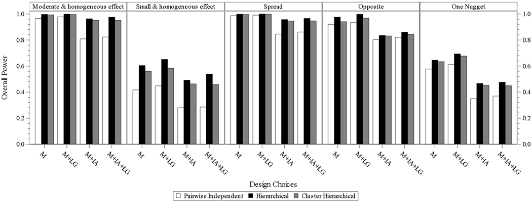
overall power for design choice under four subgroups. M = model without interim analysis and without longitudinal modelling imputation, M + LG = model without interim analysis and with longitudinal modelling imputation, M + IA = model with interim analysis and without longitudinal modelling imputation, M + IA + LG = model with interim analysis and with longitudinal modelling imputation

Fig. 3.2.

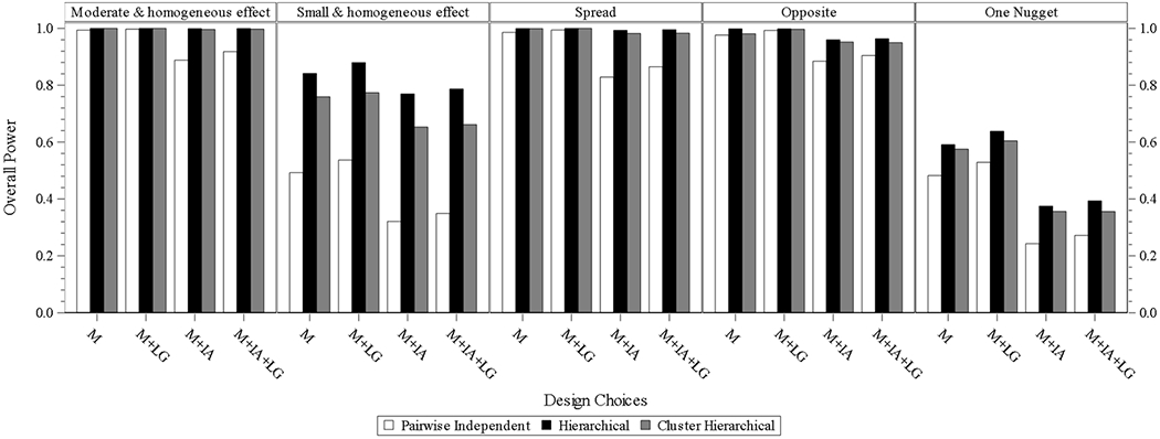
overall power for design choice under eight subgroups. M = model without interim analysis and without longitudinal modelling imputation, M + LG = model without interim analysis and with longitudinal modelling imputation, M + IA = model with interim analysis and without longitudinal modelling imputation, M + IA + LG = model with interim analysis and with longitudinal modelling imputation