Statistical Models in Clinical Studies

Abstract

Although statistical models serve as the foundation of data analysis in clinical studies, their interpretation requires sufficient understanding of the underlying statistical framework. Statistical modeling is inherently a difficult task because of the general lack of information of the nature of observable data. In this article, we aim to provide some guidance when using regression models to aid clinical researchers to better interpret results from their statistical models and to encourage investigators to collaborate with a statistician to ensure their studies are designed and analyzed appropriately.

Introduction

A statistical model is a mathematical representation of statistical assumptions about how observable data are generated. It is particularly useful for clinical studies that relate multiple variables, such as patients’ background factors, to an outcome, such as survival time, since it allows the compact representation of the relationship as a mathematical function, called a regression function. However, a statistical model is just a simplification of the true underlying relationship, and with incorrect assumptions it can easily lead to misleading results. “All models are wrong, but some are useful”; this is the famous remark by the statistician George E. P. Box [1].

Statistical modeling is inherently a difficult task because of our general lack of understanding regarding the nature of observable data, and it should be appropriately guided by clinical expertise. Another challenging aspect of statistical modeling is the underlying statistical assumptions may not be well understood by the intended audience or even the analysts [2]. This is particularly concerning as statistical software is readily available and is commonly used by researchers without appropriate expertise to perform complicated data analyses. This article thus intends to provide some basis and principles of statistical models, specifically, regression models, with the hope of helping clinical researchers to better interpret results from their statistical models, and more importantly, to strongly encourage investigators to collaborate with a statistician to ensure their studies are designed and analyzed appropriately.

Components of a Statistical Model

Statistical models are typically expressed as equations with the outcome of interest (called the dependent variable) on the left side of the equation and a set of predictors (called covariates or independent variables) on the right side, called regression models.

Outcome variables and types of regression model.

The outcome of interest can be a continuous variable, a dichotomous variable, a count variable, or a time-to-event variable. The type of outcome variable dictates the type of regression model used to analyze the data. This is because a statistical model is fit to the observed data to not only understand the relationship between the outcome and the predictors for the observed patients but to also generalize the conclusions drawn from the observed data to a larger population. The generalization is inferred from the observed data based on a set of assumptions about the probability distribution of the outcome. Table 1 summarizes the common types of outcome variables, some example outcomes, their associated probability distributions, and corresponding regression model.

Table 1.

Overview of Regression Models

	Type of outcome variable
	Continuous	Binary†	Count	Time-to-event
Examples	Weight change [3]	Objective response of complete/partial response or not [4]; Grade 3 or worse adverse event or not [4]; progression within 6 months of starting treatment or not	Number of occurrences of a rare adverse event per patient	Overall survival (OS] or Progression-free survival (PFS) times [5]
Assumed probability distribution	Normal distribution or unspecified (non-parametric)	Bernoulli or binomial	Poisson	Exponential, Weibull, and log-normal, or can be unspecified*
Common regression model	Linear regression	Logistic regression	Poisson regression	Cox proportional hazards regression
Function of outcome being modelled	The mean	Odds, (=P/(1 – P)) or Log(odds) (= log(P/(1 – P))**	Expected count (e.g., expected number of adverse events per patient)	Hazard rate (e.g., hazard rate of mortality for OS, of death or disease progression for PFS)

^†Binary variables are frequently transformed from multinominal variables (such as cancer types] or ordinal variables (such as disease severities or grades] by introducing a grouping or threshold. Alternatively, such variables can be modeled based on extensions of logistic models, i.e., multinominal logistic models and ordinal logistic models (such as adjacent-category logistic models and cumulative or proportional-odds models] [6].

^*The Cox regression is semi-parametric since the particular distributional form of the time-to-event distribution (or survival distribution] is unspecified, while the particular form of predictor effects is specified for the hazard rate.

^**P = probability of success

Examples of outcome types and regression models in lung cancer literature include: weight change (continuous variable) from the start of cancer therapy in non-small-cell lung cancer (NSCLC) patients was modeled using linear regression [3]; objective overall response rate (ORR, binary variable), grade 3 or worse adverse events (binary) after treatment of gemcitabine and carboplatin with or without cediranib as first-line therapy in advanced NSCLC were evaluated using logistic regression models [4]; and overall survival (OS, time-to-event) and progression-free survival (PFS, time-to-event) in patients with advanced NSCLC treated with PD-1/PD-L1 check-point inhibitors were evaluated using Cox proportional hazards models [5].

Predictor variables and interpretation.

The predictors in a regression model can be categorical or continuous variables. The simplest categorical predictor has two levels, for example, sex (male vs. female). A linear regression model evaluating the association between sex and weight loss [3] can be stated as Mean(weight loss) = α + β · sex where female is the reference category (sex = 0) and sex = 1 represent male. In this model the intercept α represents the mean weight loss of female patients, while the β represents the difference in mean weight loss between male and female patients. A positive β means, on average, male patients lost more weight than female patients whereas a negative β means, on average, male patients lost less weight than female patients.

In general, a categorical predictor with K categories is represented by K-1 dummy variables, i.e., binary (0/1) variables, in a regression model with one category serving as the reference. For example, a model evaluating the association post-treatment weight loss and body mass index (BMI, categorized as 4 groups: underweight, normal weight, overweight, or obese) at the start of chemotherapy can be stated as Mean(weight loss) = α + γ₁ · bmi₁ + γ₂ · bmi₂ + γ₃ · bmi₃, where normal weight is the reference category and bmi₁ = 1 for underweight and bmi₁ = 0 otherwise, bmi₂ = 1 for overweight and bmi₂ = 0 otherwise, and bmi₃ = 1 for obese and bmi₃ = 0 otherwise. The α is the mean weight for patients with normal weight and γ₁, γ₂, γ₃ are the differences in mean weight between patients who are underweight, overweight, and obese compared to patients with normal weight.

For a continuous predictor, e.g., age at baseline in years, its association with the outcome can be evaluated in the linear model, Mean(weight loss) = α + ϕ · age. The intercept α represents Mean(weight loss) at age = 0 and ϕ represents the change in mean weight loss with every year increase in age. However, it is worth noting that age = 0 may be far outside the range of the study population, and one can avoid such an extrapolation by introducing a typical age level, such as 50, as the reference age, by subtracting 50 from age. In this case, the model can be expressed as Mean(weight loss) = α + ϕ · (age – 50), where α now represents Mean(weight loss) at age = 50. In some cases, when ϕ, the change in one-year increment is deemed negligibly small, it is more meaningful to consider the effect of a substantial change in age, such as 10 years. As such, one may work with a modified predictor, age_trans = (age – 50)/10, and assume Mean(weight loss) = α + ϕ · age_trans, where ϕ now represents the change in mean weight loss associated with every 10-years increase in age.

This example assumes that the effect of age is linear, i.e., the incremental impact on mean weight loss associated with each year increase in age is constant over its entire range. We can check the linearity assumption simply based on a scatter plot of the observed weight loss versus age in this univariable setting. Such a plot can also help in identifying outliers that can substantially influence the parameter estimation (see Section “Univariable versus Multivariable Models” for related plots and detection of influential observations in the multivariable setting). When non-linearity is suggested, a more complex model should be considered, for example, a model with a quadratic effect of age, $\text{Mean}(\text{weight loss})=\alpha +{\varphi }_1\cdot {\text{age}}_{\mathrm{trans}}+{\varphi }_2\cdot {\text{age}}_{\mathrm{trans}}^2$. More flexible splines and other non-parametric models are also available [7]. Another approach address non-linearity is transformation of the outcome variable, such as log transformation. This approach can also help to yield a distribution that is nearer to a normal distribution with variance that is constant across the levels of the predictor variable. Alternatively, continuous predictor variables such as age are transformed into a categorical variable, e.g., less than or greater than 65 years. Such transformation may facilitate interpretation but at the cost of information loss due to grouping.

Categorical and continuous predictors are included in logistic regression models and Cox proportional hazards models in the same manner as described above for linear regression model (see Table 1). However, their associations are modeled on the log(odds) of a binary outcome and on the log(hazard rate) of a time-to-event outcome, respectively. Due to the complexity of time-to-event data analysis, Cox proportional hazards model will be covered in more details in a future article in this series.

Univariable versus Multivariable Models

So far, we have discussed models with only one predictor, often called univariable models. Such models can be extended to simultaneously include multiple predictors, called multivariable models. Most often these are referred to incorrectly as univariate and multivariate models in the clinical literature, it is important to emphasize that the appropriate terminology is univariable and multivariable models. An example of the multivariable model is:

$$\text{Mean}(\text{weight loss})=\alpha +{\beta }_1\cdot \text{sex}+{\beta }_2\cdot {\mathit{bmi}}_1+{\beta }_3\cdot {\mathit{bmi}}_2+{\beta }_4\cdot {\mathit{bmi}}_3+{\beta }_5\cdot {\text{age}}_{\mathrm{trans}},$$ (1)

where sex, bmi, and age_trans are defined as in previous models. Here, the intercept α represents the mean weight loss of a female patient with normal weight whose age is 50, corresponding to age_trans = (age – 50)/10 = 0. However, interpretation of the regression parameters β’s is now conditional on the values of the other predictors. For example, β₁ represents the difference in mean weight loss of a male patient compared to a female patient in the same BMI category and the same age. Similarly, β₂ represents the difference in mean weight loss of an underweight patient compared to a normal weight patient the same sex and age category. More generally, the effect of each predictor in the above multivariable model compares the outcome of individuals with the same attributes except for the predictor being evaluated. This aspect of multivariable models is particularly useful when adjusting for confounding factors. Here, confounding represents the effect of treatment which is not distinguishable from those of other factors, called confounding factors, which typically relate to both the treatment selection and the outcome variable, but are not mediators of the treatment effect on the outcome. Multivariable models allow for evaluation of the treatment effect conditional on the same attributes of confounding factors by including them as predictors.

Another aspect of the above multivariable model is that the effect of a predictor is the same regardless of the value of the other predictors. For example, the effect of sex β₁ on mean weight loss is constant irrespective of the BMI levels or age (see Fig 1A). This assumption can be relaxed by introducing an interaction term, such as sex × age_trans. Specifically,

$$\text{Mean}(\text{weight loss})=\alpha +{\beta }_1\cdot \text{sex}+{\beta }_2\cdot {\mathit{bmi}}_1+{\beta }_3\cdot {\mathit{bmi}}_2+{\beta }_4\cdot {\mathit{bmi}}_3+{\beta }_5\cdot {\text{age}}_{\mathit{trans}}+{\beta }_6\cdot (\text{sex}\times {\text{age}}_{\mathit{trans}}),$$ (2)

which allows for differential effect of sex on mean weight loss across the levels of age (see Fig 1B). Inclusion of interaction terms should be considered to capture effect modifications between predictors, even though it can make a model and its interpretation more complex.

Fig 1.

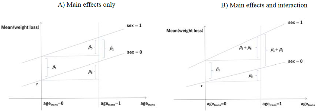
Multivariable models without interaction (A) and with interaction (B). In the multivariable model with main effects only given in Equation (1) (panel A), two regression lines are parallel, indicating constancy of sex effect for any value of age (i.e., β₁) and constancy of age effect for any value of sex (i.e., β₅) in subjects with a given level of BMI. On the other hand, in the multivariable model with interaction given in Equation (2) (panel B) the regression lines are not parallel, and the effect of sex now depends on age and vice versa; the effect of sex for age = 50 or age_trans = (age – 50)/10 = 0 is β₁, but that for age_trans =1 is β₁+β₆. Similar interpretation applies to the effect of age for each sex category.

We have thus far considered additive effect models. The advantages of this type of model are ease of interpretation and suitability for evaluating absolute effects of factors or interventions in a population. However, additive effect models can suffer from technical issues, especially for non-continuous outcome variables, and models with multiplicative effects, such as logistic, Poisson, Cox regression models, can be considered (see Table 1).

Model Complexity versus Data Information

Generally, statistical models become complex as the number of parameters (β’s) increases, e.g., by entering many predictors, possibly including non-linear or interaction terms, in the regression model. However, a complex model will not work when it is fit to a dataset that does not contain enough information to estimate the parameters. The limiting sample size represents the amount of data information required for model fitting, typically measured by the number of subjects for continuous outcome variables and by the number of events in the analysis of censored time-to-event data (see Table 1).

In regression modeling, there are rules for limiting sample size, such as “at least 10 subjects per predictor.” [8] However, it should be noted that these are crude criteria that do not take into account the joint distribution among variables, such as multicollinearity, which represents high correlations among predictors and multivariable models must be free of multicollinearity for independent predictors. An estimation that is unstable due to lack of limiting sample size, multicollinearity, or other reasons can be recognized by unrealistic parameter estimates or confidence intervals and/or by warning messages from the statistical software indicating that the estimates or the variances cannot be obtained.

Modeling for Effect Assessment versus Modeling for Classification/Prediction

The strategy for regression modeling depends on the intended use of the model. Two common uses of statistical models are effect assessment and risk classification or prediction. If the model is used to assess the treatment effect or the impact of a risk factor, it is important that the model provides unbiased estimates of the treatment effect or impact of the risk factor of interest after adjusting for established prognostic factors and confounding factors. As such, careful selection of predictors based on both statistical and clinical perspectives is warranted. Various variable selection techniques and their implications can be found in statistical literature [8–11].

It must be emphasized that model checking and diagnostics are critical. For example, in the multivariable linear model of mean weight loss, the linearity assumption for a continuous predictor, e.g., age, can be checked by a scatter plot of the residual versus age, where the residual for a patient is defined as the observed weight loss minus the fitted weight loss for that patient. Another aspect of model diagnostics is identification of influential observations, representing patients or groups of patients with particular predictor profiles, in estimating respective regression coefficients. Specifically, when the change of a regression coefficient estimate after deleting certain observations, called delta-beta, is substantial, it would be regarded as influential in estimating the regression coefficient. As a more theoretical remark, a linear model for a continuous outcome variable requires four main assumptions: linearity, independence [observations are independent from each other), normality [residuals follow a normal distribution), and homoscedasticity of residuals across the levels of the predictors, although the linear regression is relatively robust to deviations in the latter two assumptions. In case where different regression models with different sets of predictors or from different sets of observations are considered important, it would probably be wise to present the results of all these models. This is helpful to evaluate the robustness of the main results or conclusions from the regression analysis to different regression models as a sensitivity analysis.

If the regression model is intended to be used as a scoring system for risk classification or for prediction, then the overall prediction accuracy of the model – as measured by sensitivity, specificity, the C-statistic for classification and the Hosmer-Lemeshow statistic and Brier score for prediction [12] – is more important than providing unbiased estimate for each predictor in the model. For example, Mandrekar et al. [13] developed a prognostic model for advanced NSCLC and assessed its accuracy in classifying prognostic risk using the C-statistic, which represents the probability that a randomly selected patient who develops an event of interest has a higher risk score than a patient who had not developed the event.

In classification or prediction, the estimates of β’s are regarded simply as weights, rather than effects, and will be tuned to achieve high prediction accuracy. For the standard regression models, such as linear, logistic, Poisson, and Cox regression models [see Table 1), penalized regressions, such as ridge and lasso [14,15], are a technique to shrink the regression parameters or weights toward zero. The resultant weights are thus biased, but more stable (i.e., less variance). As the penalization reduces the number of parameters [the degree of freedom) substantially in the process of estimation by shrinkage, it is effective especially when the number of predictors or parameters is large relative to the limiting sample size.

All regression models are subject to overfitting to random noise, rather than systemic variation in the data used to build the model [8,14,16]. In classification or prediction, resampling techniques, such as split-sample, cross-validation, or bootstrap, can be used for internal validation to assess the accuracy using the study population for which the model was developed [17]. However, an external validation study using an independent set of samples is generally warranted. See the TRIPOD guidelines for reporting both model building and validation studies [17].

Concluding Remarks

In this article, our focus is on the basis and principles of statistical models after collection of a dataset for statistical analysis. We emphasize that the key to successful data analyses is designing the study to enhance the quality and quantity of data relevant to the study objective [18–20].

References

- 1.Box GEP, Draper NR. Empirical model-building and response surfaces. New York, USA: Wiley; 1987. [Google Scholar]
- 2.Greenland S Introduction to regression models. In Rothman KJ, Greenland S, Lash TL, eds. Modern Epidemiology, 3rd edn. Philadelphia, USA: Lippincott Williams & Wikins; 2008, pp. 381–417. [Google Scholar]
- 3.Le-Rademacher J, Lopez C, Wolfe E, Foster NR, Mandrekar SJ, Wang X, Kumar R, Adjei A, Jatoi A. Weight loss over time and survival: a landmark analysis of 1000+ prospectively treated and monitored lung cancer patients. J Cachexia Sarcopenia Muscle. 2020. doi: 10.1002/jcsm.12625. [DOI] [PMC free article] [PubMed] [Google Scholar]
- 4.Dy GK, Mandrekar SJ, Nelson GD, Meyers JP, Adjei AA, Ross HJ, Ansari RH, Lyss AP, Stella PJ, Schild SE, Molina JR, Adjei AA. A randomized phase II study of gemcitabine and carboplatin with or without cediranib as first-line therapy in advanced non-small-cell lung cancer: North Central Cancer Treatment Group Study N0528. J Thorac Oncol. 2013; 8: 79–88. [DOI] [PMC free article] [PubMed] [Google Scholar]
- 5.Negrao MV, Lam VK, Reuben A, Rubin ML, Landry LL, Roarty EB, Rinsurongkawong W, Lewis J, Roth JA, Swisher SG, Gibbons DL, Wistuba II, Papadimitrakopoulou V, Glisson BS, Blumenschein GR Jr, Lee JJ, Heymach JV, Zhang J. PD-L1 expression, tumor mutational burden, and cancer gene mutations are stronger predictors of benefit from immune checkpoint blockade than HLA class I genotype in non-small cell lung cancer. J Thorac Oncol. 2019; 14: 1021–1031. [DOI] [PubMed] [Google Scholar]
- 6.Hosmer DW, Lemeshow S, Sturdivant RX. Applied Logistic Regression, 3rd edn. Wiley; 2013. [Google Scholar]
- 7.Hastie TJ, Tibshirani RJ. Generalized Additive Models. Boca Raton, USA: Chapman & Hall/CRC; 1990. [Google Scholar]
- 8.Harrell FE. Regression Modeling Strategies With Applications to Linear Models, Logistic and Ordinal Regression, and Survival Analysis. Springer; 2015. [Google Scholar]
- 9.Greenland S, Pearl J, Robins JM. Causal diagrams for epidemiologic research. Epidemiology 1999; 10: 37–48. [PubMed] [Google Scholar]
- 10.Williamson EJ, Aitken Z, Lawrie J, Dharmage SC, Burgess JA, Forbes AB. Introduction to causal diagrams for confounder selection. Respirology 2014; 19: 303–311. [DOI] [PubMed] [Google Scholar]
- 11.Heinze G, Dunkler D. Five myths about variable selection. Transpl Int. 2017; 30: 6–10. [DOI] [PubMed] [Google Scholar]
- 12.Steyerberg EW, Vickers AJ, Cook NR, Gerds T, Gonen M, Obuchowski N, Pencina MJ, Rattan MW. Assessing the performance of prediction models: a framework for traditional and novel measures. Epidemiology 2010; 21: 128–138. [DOI] [PMC free article] [PubMed] [Google Scholar]
- 13.Mandrekar SJ, Schild SE, Hillman SL, et al. A prognostic model for advanced stage nonsmall cell lung cancer pooled analysis of north central cancer treatment group trials. Cancer 2006: 107:781–92. [DOI] [PubMed] [Google Scholar]
- 14.Hastie T, Tibshirani R, Friedman J. The Elements of Statistical Learning: Data Mining, Inference, and Prediction. 2nd edn. Springer; 2009. [Google Scholar]
- 15.Halabi S, Li C, Luo S. Developing and validating risk assessment models of clinical outcomes in modern oncology. JCO Precis Oncol. 2019; 3: 10.1200/P0.19.00068. [DOI] [PMC free article] [PubMed] [Google Scholar]
- 16.Babyak MA. What you see may not be what you get: a brief, nontechnical introduction to overfitting in regression-type models. Psychosom Med. 2004; 66: 411–421. [DOI] [PubMed] [Google Scholar]
- 17.Moons KG, Altman DG, Reitsma JB, Ioannidis JP, Macaskill P, Steyerberg EW, Vickers AJ, Ransohoff DF, Collins GS. Transparent Reporting of a multivariable prediction model for Individual Prognosis or Diagnosis (TRIPOD): explanation and elaboration. Ann Intern Med. 2015; 162: Wl–73. [DOI] [PubMed] [Google Scholar]
- 18.Hernán MA, Robins JM. Using big data to emulate a target trial when a randomized trial is not available. Am J Epidemiol. 2016; 183: 758–764. [DOI] [PMC free article] [PubMed] [Google Scholar]
- 19.Steyerberg EW. Clinical Prediction Models: A Practical Approach to Development, Validation, and Updating. 2nd edn. Springer; 2019. [Google Scholar]
- 20.Riley RD, Ensor J, Snell KIE, Harrell FE Jr, Martin GP, Reitsma JB, Moons KGM, Collins G, van Smeden M. Calculating the sample size required for developing a clinical prediction model. BMJ. 2020; 368: m441. [DOI] [PubMed] [Google Scholar]