

Abstract
A hydrodynamic/acoustic splitting method was used to examine the effect of supraglottal acoustics on fluid–structure interactions during human voice production in a two-dimensional computational model. The accuracy of the method in simulating compressible flows in typical human airway conditions was verified by comparing it to full compressible flow simulations. The method was coupled with a three-mass model of vocal fold lateral motion to simulate fluid–structure interactions during human voice production. By separating the acoustic perturbation components of the airflow, the method allows isolation of the role of supraglottal acoustics in fluid–structure interactions. The results showed that an acoustic resonance between a higher harmonic of the sound source and the first formant of the supraglottal tract occurred during normal human phonation when the fundamental frequency was much lower than the formants. The resonance resulted in acoustic pressure perturbation at the glottis which was of the same order as the incompressible flow pressure and found to affect vocal fold vibrations and glottal flow rate waveform. Specifically, the acoustic perturbation delayed the opening of the glottis, reduced the vertical phase difference of vocal fold vibrations, decreased flow rate and maximum flow deceleration rate (MFDR) at the glottal exit; yet, they had little effect on glottal opening. The results imply that the sound generation in the glottis and acoustic resonance in the supraglottal tract are coupled processes during human voice production and computer modeling of vocal fold vibrations needs to include supraglottal acoustics for accurate predictions.
Introduction
Voiced sound production in the human larynx is a complex three-way interaction between glottal aerodynamics, vocal fold vibration, and supraglottal acoustics. The airflow from the lungs interacts with vocal fold tissues to initiate sustained vibrations, which modulate the airflow to form a sound source. The sound source subsequently passes through the supraglottal tract which primarily serves as an acoustic resonator to reshape the spectrum of the source to form a specific vowel or consonant. Following Titze [1], the source-acoustics interaction is generally categorized into two levels. Level 1 is described in which vocal fold vibrations are not significantly disturbed by the supraglottal acoustics. This level usually occurs in low-moderate pitch speech, when the dominant harmonics are well below the formants of the supraglottal vocal tract so that only the higher harmonics interact with the formants. These higher harmonics often do not have a significant influence on vocal fold vibrations. Level 2 is described in which vocal fold vibrations are significantly disturbed by the supraglottal acoustics so it involves a change of vibration pattern. This level occurs in high-pitch speech and even more in singing when the dominant harmonics are near the formants. Source instabilities, such as bifurcation, subharmonic frequencies, sudden F0 jumps, or chaotic vibrations, were observed to occur in this level [1–10].
Normal speech production is generally at the low-moderate pitch, so the source-filter interaction is considered mild. For this reason, computer modeling of voice production often treats sound source generation and acoustic resonance as separate processes. For example, the Bernoulli's equation, which assumes a one-dimensional, inviscid and incompressible flow, was often used to model glottal aerodynamics during fluid–structure interactions without including supraglottal acoustics. If needed, an additional one-dimensional wave equation would be used for modeling the acoustics, yet in most cases in a one-way coupling [1,11–14]. In high-fidelity modeling, ideally, solving the fully compressible Navier–Stokes equations in the entire domain of the larynx and supraglottal tract would inherently include the effect of acoustics on fluid–structure interactions. Several studies have attempted to use this approach [15–18]; yet, the Mach number of the glottal airflow is about 0.1 and solving the fully compressible Navier–Stokes equations to resolve both the flow and acoustic fields simultaneously at this low Mach number is very costly. Thus, most models only employed the incompressible Navier–Stokes equations to model the fluid–structure interactions [19] and used either acoustic analogy or hydrodynamic/acoustic splitting method to model the supraglottal acoustics [20]; yet, they only considered one-way coupling in which the supraglottal acoustics was not fed back to the incompressible flow model and vocal fold vibration model [21–24].
A few past studies, however, suggested that the supraglottal acoustics may play an important role in fluid–structure interactions. For instance, Zañartu et al. [25] coupled a one-mass vocal fold model, the Bernoulli equation and the one-dimensional wave equation to investigate the relative importance of the tract acoustic loading and time-varying flow resistance in fluid–structure energy transfer. They found that for both mild and strong source-acoustics interactions, the acoustic loading contributed more significantly to the net energy transfer than the time-varying flow resistance. Another study [15] using the Navier–Stokes equation to simulate fluid–structure interactions found that ignoring the effect of supraglottal acoustics could fail to reach self-sustained vibrations while considering the effect can yield sustained steady vibrations with the same vocal fold conditions. In a computational study using the hydrodynamics/acoustic splitting method to model human voice production [26], it was found that acoustic perturbation pressure at the glottis had the same order of magnitude as the incompressible flow pressure.
While the potential role of the supraglottal acoustics in fluid–structure interaction during normal voice production was suggested, the understanding is not complete. This study aimed to improve the understanding by using a hydrodynamic-acoustic method based voice production model which separates the acoustic perturbation components of the airflow and allows a direct assessment of the effect of supraglottal acoustics on fluid–structure interactions. The hydrodynamic/acoustic splitting method decomposes the total flow variables into incompressible variables and perturbed compressible ones and in this way splits the original compressible Navier–Stokes equations into the incompressible Navier–Stokes equations and linearized perturbed compressible equations (LPCEs). The incompressible Navier–Stokes equations compute the viscous flow field, and the linearized perturbed compressible equations compute the acoustic field. By separating the viscous incompressible flow and acoustics, the method resolves the issue of scale disparity in low Mach number aeroacoustics and meanwhile allows a direct assessment of the effect of aeroacoustics. The method has been extensively validated for many canonical problems [27].
In this study, the accuracy of the splitting method in simulating compressible flows in typical human airway configurations was first verified by comparing to fully compressible Navier–Stokes equation simulations using the commercial software ansys fluent. The splitting method was then coupled with a three-mass model of vocal fold vibrations to simulate fluid–structure interactions during normal voice production. Two simulation cases, one with the supraglottic acoustic coupled with the vocal fold vibration model and the other without, were simulated. The predicted glottal flow rate waveform, vocal fold vibration amplitude and patterns, and aerodynamic loadings were extensively compared between the two cases to evaluate the effect of supraglottal acoustic on fluid–structure interactions.
Methods
The hydrodynamic/acoustic splitting method divides the total flow variables into the incompressible components and perturbed compressible ones as follows:
| (1) |
where and , respectively, are the total flow velocity and pressures, and , respectively, are the acoustic perturbed velocity and pressure, and and , respectively, are the incompressible velocity and pressure. Substituting the above relationship into the fully compressible Navier–Stokes equation and following the linearization method of Seo and Moon [27], the compressible Navier–Stokes equations can be divided into incompressible Navier–Stokes equations and LPCEs. At each time-step, the incompressible Navier–Stokes equations are first solved, and then LPCE is solved based on the incompressible Navier–Stokes equations solution. The total velocity and pressure variables are at last obtained using Eq. (1). This hybrid approach has been validated comprehensively for canonical problems [22,27] at low Mach numbers and successfully utilized to model human phonation [22]. The numerical methods for solving these equations are described below.
Incompressible Flow Model.
The incompressible Navier–Stokes equations are
| (2) |
where and are the incompressible flow density and kinematic viscosity, respectively.
An in-house immersed-boundary method based solver [28] was developed to solve the equations. The incompressible Naiver Stokes equations are discretized in space using a second-order central difference scheme with a cell-centered, collocated arrangement of the primitive variables, (). In addition to the cell center velocities, the face-center velocities, , are computed and updated separately to improve the mass conservation. A fractional time-step scheme is used to integrate the equation in time which consists of three substeps. In the first substep, the modified momentum equation without pressure term is solved to obtain the intermediate velocities. A second-order Adams–Bashforth scheme is employed for the convective terms while the implicit Crank–Nicholson scheme is used to discretize the diffusion terms to eliminate the viscous stability constraint. The second step solves a pressure Poisson equation to obtain the pressure field. In the final step, the velocity field is updated to its final values based on the updated pressure. The immersed boundary is treated using a ghost cell methodology, which satisfies the boundary condition at the extract location, and has a second-order accuracy both globally and near the immersed boundaries. The detailed information can be found in Zheng et al. [29] and Mittal et al. [28].
Acoustics Model.
The LPCE [27] are
| (3) |
where is the ratio of the specific heats. An in-house solver was used to solve the equations. In the solver, the equations are discretized with a sixth-order central compact finite difference scheme in space and integrated using a four-stage Runge–Kutta (RK4) method in time. A high-order weighted least-squares ghost cell immersed-boundary method was implemented to deal with complex moving boundaries. Further details of this model can be found in Ref. [27].
Vocal Fold Model.
A classic three-mass vocal fold model [30] was used to simulate vocal fold dynamics. In this model, three lumped masses are used to represent the body and cover layers of the vocal fold, and they are connected via springs and dampers. Figure 1(a) shows a schematic structure of the three-mass model, in which , , and , represent the mass, spring and damping coefficients of the upper portion of the cover layer, respectively, and , , and , represent the corresponding values of the lower portion of the cover layer. The two masses are coupled by a spring with stiffness of . , , and represent the corresponding values of the body layer. All of the three masses are only allowed to move in the lateral direction.
Fig. 1.
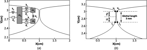
(a) Schematic of the three-mass vocal fold model, and are the spring coefficients and damping constants for different masses, . (b) Zoom-in view of the glottis. , and represent the two top points on the left and right vocal folds, respectively, while and represent the two corresponding points on the bottom. and represent the thickness of the upper and lower mass, respectively.
The differential equations of the three-mass model are
| (4) |
where , , and are the current position of the three masses in the medial–lateral direction, , , and are the nonlinear coefficients for the three masses, and are the loads on the upper and lower mass in the medial–lateral direction, respectively. In the current simulation, , , and were set to be 100 [30], and the damping coefficients , , and were computed with the following equations:
| (5) |
where = 0.2, = 0.4, and = 0.2.
The differential equations were solved using a fourth-stage Runge–Kutta method. The parameters in the three-mass model were taken from Story and Titze [30] and listed in Table 1.
Table 1.
Parameters of the three-mass vocal fold model [30]
| Parameters | |||||||||
|---|---|---|---|---|---|---|---|---|---|
| Value | 0.01 | 0.01 | 0.05 | 3.5 | 5.0 | 20.0 | 0.5 | 0.15 | 0.15 |
Fluid–Structure–Acoustics Coupling.
The hydrodynamic/acoustic splitting model and vocal fold model were strongly coupled to simulate fluid–structure interactions. The interaction took place at the vocal fold surface through marker points, as shown in Fig. 1(b). At each time-step, the vocal fold model provided the updated velocity and location of the vocal fold surface as the boundary conditions for the incompressible flow and LPCE solvers to compute the incompressible flow field and acoustic perturbation field. For the case including the supraglottal acoustics, both the incompressible flow pressure and acoustic pressure were then applied at the vocal fold surface to compute vocal fold deformations. For the case without the supraglottal acoustics, only the incompressible flow pressure was then applied at the vocal fold surface to compute vocal fold deformations. As shown in Fig. 1(b), the velocities of the inferior marker point-pair, and , and the superior marker point-pair, and , were directly obtained from the vocal fold model. The velocities of other marker points were computed through linear interpolations.
The forces acting on the two masses ( and ) were computed by integrating the pressure () on the vocal fold surface
| (6) |
where is the lower bound of location of the lower mass in inferior–superior direction, x represents the medial–lateral direction, and y represents the inferior–superior direction. In this study, , , and . Since the masses could only move in the medial–lateral direction, forces in the inferior–superior direction are neglected.
Results and Discussion
Verification.
The incompressible flow model and vocal fold model, as well as their coupling have been extensively verified in previous studies [28,31–35]. This study focused on the verification of using the splitting method in simulating compressible flows in the human vocal tract. Three cases with the geometric configurations and boundary conditions relevant to the human vocal tract were simulated. A compressible flow solver of the commercial software ansys fluent was also used for the simulations. The results from the two solvers were compared for verification.
Case 1: A Straight Duct with Pulsating Velocity Inlet.
The compressible Navier–Stokes solver in Fluent applies the Roe-FDS convective flux to the implicit formulation. The equations are discretized using the third-order-MUSCL scheme. Figure 2(a) shows the simulation setup in fluent, which followed the work of Zhang et al. [15]. They used the same case to verify the accuracy of a slightly compressible flow solver in simulating fluid–structure interactions during voice production. A straight duct with the dimensions of 17.3 cm in length and 2.8 cm in width and with a pulsating velocity inlet was simulated. A zoomed-in view of the duct is provided in Fig. 2(a), which was discretized using 15,000 () grids uniformly distributed in each direction. A large half-circle domain with a radius of 1000 cm was used as the far-field domain. This large radius is chosen to delay the feedback of the reflected waves from the far-field domain. 30,450 structured grid elements were used in the far-field domain with the coarsest grid near the outer boundaries and densest grid near the duct exit with a stretch ratio of 1.05. A finer grid with 137,115 elements was used for the grid independence test, and it resulted in less than 1% of the average difference based on the total flow rate at the duct exit. At the outer boundaries of the far-field domain, a zero-gauge pressure outlet boundary condition was applied. A time-step of was employed to be consistent with Zhang et al. [15] and also to ensure the Courant–Friedrichs–Lewy (CFL) stability constraint below 1.
Fig. 2.

Computational domain and boundary conditions of case 1 for (a) the compressible flow simulation in fluent and (b) the splitting method
Figure 2(b) shows the simulation setup in the splitting method solver. The dimensions of the duct were the same as those in the Fluent simulation. The duct was discretized using 60,000 () Cartesian grids uniformly distributed in each direction. Different from the fluent simulation which used a large half-circle far-field domain, the splitting method used a square far-field domain. The acoustic reflection of the outer boundaries was eliminated by enforcing anechoic zones using buffers (Fig. 2(b)) [36] in the ten outer grid cells in each direction. The far-field domain was discretized using 57,344 () nonuniform cartesian grid elements with the coarsest grid near the outer boundaries and the densest grid located near the duct exit with a stretch ratio of 1.08. A grid independence study was conducted by using a finer grid resolution of a total of 469,376 grid elements. The results showed an average difference of 3.7% based on the total flow rate at the duct exit. To satisfy the CFL constraint of below 1, a time-step of was used for the incompressible solver, and a time-step of was employed for the LPCE solver.
A Gaussian pulse wave () [15] was used as a velocity inlet boundary condition to generate a pulsatile flow for the Fluent simulation. This velocity wave was also applied as the incompressible inlet velocity in the splitting method. By employing Eq. (1), the inlet velocity of the LPCE solver will be zero.
Figure 3 shows the pressure contour inside the duct and far-field domain at five different time instants simulated by the splitting method. The unfilled and filled arrows indicate the incident and reflected pressure waves at mouth, respectively. The compressible flow simulation in Fluent showed the same pattern and values. The sound speed predicted by the splitting method was 329 m/s, which agreed well with the compressible flow simulation, which predicted 330 m/s.
Fig. 3.

Snapshots of the incident and reflected pressure waves from the inlet and exit of the duct at different instances. The filled and unfilled arrows indicate the incident and reflected pressure waves at mouth, respectively.
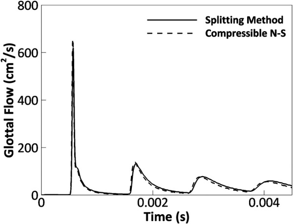
Figure 4 shows the time history of the volume flow rate at the exit of the duct simulated by the splitting method and compressible flow solver. The two solvers agreed well with an average difference of 2.0%.
Fig. 4.

Comparison of the volumetric flow rate at the exit of the duct predicted by the splitting method and compressible flow simulation for case 1
Case 2: A Straight Duct with Pulsating Pressure Inlet.
To verify the splitting method for simulating pressure boundary conditions, case 2 was created by applying a pressure Gaussian pulse wave () at the inlet. Figure 5 compares the volumetric flow rate at the exit of the duct predicted by the splitting method and compressible flow simulation. The curves showed a good agreement in terms of shape and peak values. The average error was 8.1% with the maximum error occurring at the first peak (5.6% error). The relatively large error of the averaged flow rate was due to a slight phase difference between the two curves. Moreover, the smoothing of acoustic pressure peaks is likely due to the viscous flow effects which smooth the sharp peaks.
Fig. 5.
The comparison of the volumetric flow rate at the exit of the duct predicted by the splitting method and compressible flow simulation in case 2
Case 3: A Straight Duct with a Small Gap and Periodic Velocity Inlet.
To include the effects of the presence of vocal folds, two rectangular obstacles were added to the duct with a small gap of 3 mm to represent the typical size of the human glottal gap (Fig. 6). To represent the effect of vocal fold vibration on modulating the airflow, a periodic velocity profile was used at the inlet (Fig. 6). The velocity profile was generated by following the glottal flow model of the Liljencrants–Fant model [37]. In this model, the time derivative of the flow rate over one cycle is as follows:
| (7) |
Fig. 6.

The details of the subglottal duct and glottal gap in case 3. The subfigure shows the periodic velocity profile applied at the inlet.
where , , , , , is a typical period of a cycle for an adult male glottal flow rate.
The volumetric flow rate at the exit of the duct predicted by the splitting method and compressible flow simulation is shown in Fig. 7. The two methods showed a good agreement with the average difference of 5.6%. It was noticed that the shape of flow rate waveform at the exit differed significantly from that at the inlet, indicating a strong effect of the acoustic perturbation on altering the flow rate at the exit. It was also noticed that the flow rate at the exit had significant negative peaks which did not exist at the inlet. These strong negative flow rates at the exit were the results of strong acoustic pressure oscillations.
Fig. 7.

The comparison of the volumetric flow rate at the exit of the duct predicted by the splitting method and compressible flow simulation in case 3
In summary, the splitting method showed a good agreement with the compressible flow simulation for low-Mach number internal flow problems with both velocity and pressure boundary conditions. For the three verification cases that represent typical human voice production conditions, the average differences between the two methods in predicting the flow rate ranged between 2.0% and 8.1%. The verification provides the confidence of using the splitting method to investigate the effect of supraglottal acoustics on fluid–structure interactions during human voice production. It is noted that both the splitting method and compressible flow simulation predicted strong acoustic perturbations in the duct, which significantly altered the shape of the flow rate waveform at the exit of the duct.
Effects of Supgraglottal Acoustics on Fluid–Structure Interactions
Simulation Cases.
This session compares the results of two simulation cases, one with the acoustic solver coupled with the vocal fold model (denoted as (+) acoustics) and the other without (denoted as (−) acoustics). The effects of the supraglottal acoustics on the glottal flow rate, vocal fold vibration and aerodynamic loading on the vocal folds are discussed. The simulation setup is described below.
A two-dimensional straight channel was used as a simplified shape of the vocal tract. The entire tract was 20 cm long with 17.4 cm in the supraglottal portion [38] and 2.0 cm in the subglottal portion (shown in Fig. 8). The profiles of the true and false vocal folds were taken from Zheng et al. [39], which was reconstructed from a thin-slice CT scan of a male larynx. The airway was immersed into a rectangular box, and a far-field domain was added on top of the box to capture the radiation effects at the mouth. The detailed dimensions are shown in Fig. 8. To deal with the contact of the vocal folds, a kinematic constraint was applied to enforce a minimum glottal gap of 0.02 cm, which was about 7% of the maximum glottal gap during vibration.
Fig. 8.

The computational domain, profiles of the vocal folds (VFs) and false vocal folds (FVFs), mesh arrangement and boundary conditions of the fluid–structure interaction simulations
For the incompressible flow solver, a zero-gauge pressure was applied at the five outlets of the far-field domain, and a 0.8 kPa gauge pressure was applied at the inlet of the vocal tract to drive the flow. The nonpenetration nonslip boundary condition was applied on the vocal tract wall and vocal fold surface. The kinematic viscosity of the air was set as m2/s.
For the acoustics solver, the hard wall boundary condition ( and ) was applied at the vocal tract wall and vocal fold surface. To eliminate the acoustic reflection, anechoic zones were enforced by applying buffer zones (Fig. 8) [36]. The temperature of the air was assumed to be 37 °C, and the corresponding speed of sound was 351.88 m/s.
A high resolution () nonuniform Cartesian grid was used to discretize the computational domain (Fig. 8). The highest grid density was provided around the intraglottal and supraglottal regions with the maximum stretch ratio of 1.03. A grid-independence study was carried out on a grid, and the simulated key quantities were found to be grid-independent. The time history of the first two cycles has been represented in Fig. 9, which shows the agreement of both waveforms with the maximum error of 7% at t = 0.00923 s. A small time-step of ms was employed in the incompressible flow solver and solid solver, while 1/20 of this value was employed in the acoustics solver to provide a good temporal resolution as well as to satisfy the CFL stability constraint of 1. The simulations were carried out for 71,000 time-steps by a parallel simulation on 256 processors on a 6.1 TeraFLOPS cluster. The wall clock time for each simulation was about 41 h and the overall computational expense was 10,500 CPU hours.
Fig. 9.

The time history of the total flow rate of the current grids and denser grids measured at the mouth
Glottal Flow Rate.
Figure 10(a) shows the time history of the volumetric flow rate measured at the glottal exit and mouth (tract exit) for the two cases. In the (−) acoustics case, because only the incompressible nature of the flow was considered, the flow rate at the glottal exit and mouth were identical. The differences between the two cases were small at the glottal exit but large at the mouth, indicating that the acoustic perturbations had a much stronger effect on the flow rate at the mouth than that at the glottal exit due to the supraglottal tract resonance effect.
Fig. 10.

(a) The time history of the total flow rate of the two cases measured at the glottal exit and mouth. (b) The phase-averaged total flow rate of two cases measured at the glottal exit and mouth. (c) The phase-averaged total flow rate, incompressible flow rate and acoustic flow rate in the (+) acoustics case and also the incompressible flow rate in (−) acoustics case at the mouth.
Figure 10(b) shows the phase-averaged volumetric flow rate of each case measured at the glottal exit and mouth. For (+) acoustics case, the curve at the glottal exit showed a lasting flow stop during glottal closure and a ripple during flow rising, and the curve at the mouth showed a large negative peak during glottal closure and a deep depression during flow rising. These features were not observed in the (−) acoustics case which only showed smooth growing and dropping of the flow rate. Also, in the (+) acoustics case, the flow rate at the glottal exit and mouth differed significantly, indicating a presence of strong acoustic perturbations in the supraglottal tract which has significantly altered the flow rate at the mouth.
Note that past studies often considered that the primary effect of supraglottal acoustics on the flow rate waveform is to generate skewness, which is a feature that the flow rate has a longer duration of rising than dropping, resulted from the inertial effect of the air column. A skewing quotient is often used to measure the degree of skewness. It is defined as the ratio of the duration of flow acceleration to that of flow deceleration. A greater skewing quotient typically indicates a faster flow deceleration and produces a higher sound intensity [1]. This effect is different from the effect of acoustic perturbation studied in this study. The skewing effect was already included in the incompressible flow solution as the incompressible flow was solved in the entire domain of the larynx and supraglottal tract.
To specifically look at the effect of the acoustic flow rate, Fig. 10(c) plots the phase-averaged incompressible, acoustic and total flow rates at the mouth in the (+) acoustics case. The flow rate of the (−) acoustics case was also superimposed for comparison. The evaluation was chosen to be at the mouth because the difference between the two cases was most significant at the mouth. It was observed that the incompressible flow rate in the two cases was very similar, suggesting that the underlying viscous flow dynamics in the two cases were very similar. The acoustic flow rate in the (+) acoustics case oscillated around zero with the magnitude comparable to that of the incompressible flow rate. This strong acoustic flow rate has altered the shape of the total flow rate by generating a depression during flow rising and a large negative peak during glottal closure. At the glottal exit, the oscillation of the acoustic flow rate would be much lower, because the acoustic resonance in the supraglottal tract caused the acoustic flow rate to grow along the airway.
Figure 11 shows the frequency spectrum of the incompressible and acoustic flow rates at the mouth in the (+) acoustics case. It can be seen that the incompressible flow rate had the highest energy at the fundamental frequency and a very quick energy decay over the super-harmonics. The acoustic flow rate, however, had the highest energy at the third harmonics which was around 565 Hz, indicating that the strongest acoustic resonance occurred at the third harmonics. By assuming the supraglottal tract as an ideal open-closed tube, its formants can be analytically calculated as
| (8) |
Fig. 11.

The frequency spectrum of the incompressible and acoustic flow rate in (+) acoustics case at the mouth
where , is the speed of sound, and is the length of the tube [40]. By employing , , and , the first three lowest formants of the tube would be 506, 1517, and 2528 Hz. If the area variation along the tract was considered, these values would be shifted. Story and Titze [41] have calculated the formants of the current supraglottal tract shape with a frequency domain transmission line technique [42], and they found the first and second formants are 628 and 1510 Hz, respectively. Therefore, the proximity of the third harmonic with the first formant has caused the acoustic resonance.
To confirm that the resonance occurred at the first formant, the acoustic pressure versus the time along the centerline of the supraglottal tract in the (+) acoustic case is shown in Fig. 12. The pressure versus distance clearly indicates an approximate quarter standing wave in the supraglottal tract. The small fluctuations near the glottis were due to the disturbance of small near-field vortices. Also, it can be seen that the acoustic pressure had multiple waves in time and the amplitudes of the waves presented a complex fluctuation pattern.
Fig. 12.

The acoustic pressure versus time along the centerline of the supraglottal tract for the (+) acoustics case
Finally, several key quantities of the flow rate waveform at the glottal exit were computed for the two cases and listed in Table 2. In general, the supraglottal acoustics had little effect on the fundamental frequency, a non-negligible effect on the mean and maximum flow rate and a relatively larger effect on the maximum flow deceleration rate (MFDR) [14]. MFDR is defined as the maximum value of the negative slope of the glottal flow rate waveform, which positively correlates with voice intensity [14,43]. In our cases, the mean and maximum flow rate, respectively, decreased by 12.9% and 11.8%, and the MFDR decreased by 22.3% due to the supraglottal acoustics. Therefore, our results may have suggested a reduced vocal intensity due to the acoustic coupling.
Table 2.
Flow rate waveform and vocal fold dynamics related parameters computed from the two cases at the glottal exit
| Parameters | (−) Acoustics | (+) Acoustics | Difference |
|---|---|---|---|
| Flow rate waveform | |||
| (Hz) | 185 | 188 | 1.6% |
| () | 0.0459 | 0.04 | −12.9% |
| () | 0.0957 | 0.0844 | −11.8% |
| MFDR () | 196.0 | 152.3 | −22.3% |
| Vocal fold dynamics | |||
| (deg) | 45.7 deg | 9 deg | −80.3% |
| (m) | 0.00129 | 0.00139 | 7.8% |
| (m) | 0.00262 | 0.00258 | −1.5% |
is the fundamental frequency; and , respectively, are the mean and peak glottal flow rate; MFDR is the maximum flow deceleration rate; is the vertical phase difference between the upper and lower mass of the vocal fold; and , respectively, are the mean and peak glottal gap.
In summary, the simulations showed that in normal voice production when the fundamental frequency was much lower than the formants of the supraglottal tract, a strong acoustic resonance between a higher harmonic (i.e., the third harmonic in this study) and the first formant can occur. The resonance can generate strong acoustic velocity oscillations in the supraglottal tract and affect the shape of the flow rate waveform along the airway. In our simulations, the acoustic resonance had a small effect on the flow rate at the glottal exit in terms of generating a lasting flow stop during glottal closure and a small ripple during flow rising but had a strong effect on the flow rate at the mouth in terms of generating a strong negative peak during glottal closure and a deep depression during flow rising. The quantitative comparison reflected that the acoustic coupling decreased the flow rate and the maximum flow deceleration rate at the glottal exit by around 10% and 20%, respectively.
Vocal Fold Dynamics.
Figure 13(a) shows the phase-averaged glottal gap of the two cases. The glottal gap was defined as the minimum distance between two vocal folds. The rising and dropping of the glottal gap indicate the opening and closing of the glottis, respectively. The figure reflected that the acoustics did not have a noticeable effect on the maximum value and the closing phase of the glottal gap, but had a large effect on the opening phase of the glottal gap. At the beginning of the cycle when the glottal gap reached the minimum, the gap stayed at the minimum for a period in the (+) acoustics case while it immediately increased in the (−) acoustics case. It indicated that (+) acoustics case had a lasting glottal closure while the (−) acoustics didn't. Furthermore, the two cases showed a different development of the opening speed. In the (+) acoustics case, the opening was very fast at the beginning indicated by a steeper slope of the glottal gap curve and then started to slow down at about the halfway of the opening phase. In contrast, in the (−) acoustics case, the opening was very slow at the beginning and then quickly expedited, and maintained the high speed until a very late opening phase. To further confirm the observation, Fig. 13(b) plots the time rate of the change of the glottal gap for the two cases. A positive changing rate indicates the glottal opening and a negative changing rate indicates the glottal closing. The figure confirms that the highest opening speed appeared at an early opening phase in the (+) acoustics case while it appeared at a late opening phase in the (−) acoustics case. It also confirms that the changing rate of the glottis stayed at zero for a period in the (+) acoustics case corresponding to the glottal closure and the closing speed of the glottis in the two cases was nearly the same through most of the closing phase. The average and maximum glottal gap in the two cases are compared in Table 2. Because of the rounder shape of the glottal gap curve in the (+) acoustics case (Fig. 13(a)), the average glottal gap in the (+) acoustics increased about 7.8%. The maximum value only differed by 1.5%. Note that the spike on the curves close to the phase of 1 was a nonphysical behavior resulted from the contact model which enforces an artificial minimum glottal gap between the vocal folds for ensuring the success of flow simulation.
Fig. 13.

Comparison of the phase-averaged (a) glottal gap and (b) changing rate of the glottal gap, for the (+) acoustics and (−) acoustics cases
To further explore the difference of the vibratory dynamics of the vocal fold, Figs. 14(a) and 14(b) shows the phase-averaged displacement of the lower and upper masses of the vocal fold for the two cases. Only one vocal fold was studied because of the left-right symmetry. The plots reflected different vibratory dynamics of the vocal fold, especially during the early opening phase. In the (+) acoustics case, both the lower and upper masses stayed at zero displacement from phase 0 to 0.16T (T is period of the vibration), indicating that the glottis was firmly closed and no vibration occurred at any part of the vocal fold. Following the closure, the lower and up masses opened with the same speed from 0.16T to 0.44T, suggesting that the glottis was in a straight shape during this period. After that, the upper mass started to open with larger displacements, and eventually reached a higher maximum displacement than the lower mass. The upper mass reached its maximum displacement of 0.127 cm at the phase of 0.71T and the lower mass reached its maximum displacement of 0.111 cm at the phase of 0.68T. Because the glottal gap was limited by the lower displacement, it means that the glottal gap was limited by the lower mass during this period and it reached the maximum value at the phase of 0.68T. Starting from the phase of 0.44T to the end of the cycle, the upper mass had larger displacement than the lower displacement, indicating that the glottis had a divergent shape. Therefore, the glottis presented a straight shape at the early opening phase and a divergent shape through the rest of the cycle in the (+) acoustics case. In the (−) acoustics case, however, the lower mass led the upper mass through the entire vibration cycle, suggesting a convergent shape during the opening phase, a straight shape at the maximum opening and a divergent shape during the closing phase. The upper mass reached its maximum displacement of 0.129 cm at the phase of 0.76T, and the lower mass reached its maximum displacement of 0.122 cm at the phase of 0.63T. The glottal gap was limited by the upper mass during the opening phase and by the lower mass during the closing phase. The maximum glottal gap occurred when the upper and lower masses had the same displacements, which was at the phase of 0.68T. Moreover, both masses in the (−) acoustics case opened immediately after reaching the zero displacements, suggesting no clear closure at any part of the vocal fold.
Fig. 14.

The phase-averaged displacement of the lower and upper masses for the (a) (+) acoustics and (b) (−) acoustics
According to Story and Titze [30], the phase difference between the two masses () can be calculated as , where is the time delay between the two masses and is the vibration period. The phase difference between the two masses was 45.7 deg for the (−) acoustic case and 9 deg for the (+) acoustic case (Table 2). The significant reduction of the vertical phase difference in the (+) acoustics case suggested that the supraglottal acoustics tended to synchronize the motion of the two masses. It is of interest to point out that Zhang et al. [6] used a synthetic vocal fold model to study the dynamics of the acoustically driven vocal fold vibrations and aerodynamically driven vocal fold vibrations. They found that, in the acoustically driven vibrations, the lateral vocal fold motion was dominated by the in-phase motion, while, in the aerodynamic driven vibration, the lateral vocal fold motion was dominated by the out-of-phase motion. Their results suggested that the acoustic-structural coupling tended to promote the in-phase lateral motion in the vocal fold vibration, which was consistent with our finding of the more synchronized motion of the two masses with the acoustic resonance.
In summary, the acoustics showed a non-negligible effect on the vocal fold dynamics. First, it created a longer glottal closure which was not seen in the (−) acoustics case. Second, it affected the opening speed of the glottis by creating the fastest opening at an early stage while in the (−) acoustics case, the opening was slow at the beginning and become fastest at the late opening stage. Third, it reduced the phase difference of the motion of the lower and upper masses of the vocal fold, suggesting that the acoustics tended to promote the in-phase motion of the vocal fold. As a result, in the (+) acoustics case, the glottis presented a straight shape during the early opening and a divergent shape through the rest of the cycle, while, in the (−) acoustics case, the glottis presented a convergent shape during the opening, a straight shape at the maximum opening and a divergent shape during closing. Despite the above difference, the acoustics had little effect on the maximum glottal gap.
Aerodynamic Force.
In order to understand the underlying mechanism causing the dynamics difference between the two cases, it is useful to examine the force loading on the vocal fold. Figures 15(a) and 15(b) show the phase-averaged aerodynamic forces on the lower and upper masses of the vocal fold in the two cases. For the (−) acoustic case, the force was purely the incompressible flow force. For the (+) acoustic case, the force was the total of the incompressible flow force and acoustic perturbation force. To facilitate the discussion, the phase-averaged glottal gap is also plotted as the dashed line in the figures. The two cases showed very different loading curves.
Fig. 15.

Comparison of the phase-averaged total force on the lower mass and upper mass for (a) (−) acoustics and (b) (+) acoustics. (c) Comparison of phase-averaged incompressible and acoustic forces on the lower mass and upper mass for (+) acoustics. The amplitude of the glottal gap is represented on the right axis.
First, in the (−) acoustics case, the forces on both masses increased quickly from negative values to positive values at the beginning of the cycle. The positive forces would immediately push the masses apart, and consequently, the (−) acoustic case didn't show a lasting period of glottal closure. In the (+) acoustics case, however, the forces showed strong oscillations at the beginning of the cycle. For the lower mass, the force dropped from a high positive value to slightly below zero and then slowly grew to zero. For the upper mass, the force dropped to a large negative value and took a long time to grow back to zero. Therefore, for the beginning period of the cycle, the forces on the two masses were negative. These suction forces have kept the glottis in closure in the (+) acoustics case.
Second, it can be seen in the (−) acoustics case that the force on the lower mass was constantly higher than that on the upper mass during the entire glottal opening phase. This force difference has contributed to the large phase difference of the motion of the lower and upper mass. In the (+) acoustics case, however, the forces on the two masses were nearly the same for a long period until the early closing. This has contributed to the small phase difference in the motion of the two masses. It needs to be pointed out that vocal fold motion is the combined effect of the aerodynamic force and elastic force. Although the aerodynamic force was the same for the two masses in the (+) acoustics case, the elastic force would be different due to the different spring stiffness of the two masses. The small phase difference observed in the (+) acoustics case at a later stage of the opening phase was likely due to different elastic forces on the masses.
Third, the forces in the (+) acoustics case showed strong oscillations during the opening phase. The oscillations resulted in a high positive peak at the early stage of the opening phase and a valley in the middle of the opening phase, which has caused the faster opening of the glottis at the early opening phase and the quick drop of the opening rate in the middle of the opening phase in the (+) acoustics case. Due to the combined effects of the positive peak and quick drop of the force in the opening phase, the maximum glottal gap in the (+) acoustics case was nearly the same as that in the (−) acoustics case.
To single out the effect of the acoustics, Fig. 15(c) plots the phase-averaged incompressible flow force and acoustic perturbation force on the two masses in the (+) acoustics case. It was seen that the incompressible flow forces in the (+) acoustics case had similar values and trends as those in the (−) acoustics case. The acoustic forces in the (+) acoustic case oscillated around zero throughout the cycle. The peak and valley in the total forces corresponded well with the peak and valley in the acoustic forces. Therefore, the difference in the aerodynamic forces on the vocal fold between the two cases was primarily contributed by the acoustic pressure oscillations.
In summary, the (+) acoustics and (−) acoustics cases had similar incompressible flow forces on the vocal fold masses. However, the acoustic oscillations in the (+) acoustics cases caused strong acoustic perturbation forces which have significantly altered the total aerodynamic forces in the (+) acoustics case. The acoustics created negative suction forces at the very beginning of the cycle which delayed the opening of the glottis and generated a lasting period of glottal closure. The acoustic pressures also generated a high peak of the positive forces which generated faster opening of the glottis at the early opening phase. At last, the acoustic forces compensated the differences of the incompressible flow forces between the two masses, therefore reduced the phase difference of the motion of the two masses.
Conclusions
The study used the hydrodynamic/acoustic splitting method to examine the effect of supraglottal acoustics on fluid–structure interactions during normal human phonation. The accuracy of the splitting method in simulating compressible flows in typical human airway configurations was first verified by comparing to full compressible flow simulations using the commercial software ansys fluent. The results showed a good agreement with the error of the average flow rate ranging from 2% to 8.1%.
The splitting method was then coupled with a three-mass lumped vocal fold model to simulate fluid–structure interactions. By activating and deactivating the acoustic solver, two simulation cases were generated to allow an evaluation of the effects of acoustic perturbations on glottal flow waveform, vocal fold vibration and aerodynamic loading on the vocal folds.
The results showed that an acoustic resonance between a higher harmonic of the sound source and the first formant of the supraglottal tract occurred during normal human phonation when the fundamental frequency was much lower than the formants. The resonance resulted in acoustic pressure perturbations at the glottis which were of the same order as the incompressible flow pressures and found to affect vocal fold vibrations glottal flow rate waveform. Specifically, the acoustic perturbations delayed the opening of the glottis, reduced the vertical phase difference of vocal fold vibrations, decreased flow rate and maximum flow deceleration rate at the glottal exit; yet, they had little effect on glottal opening. The results imply that the sound generation in the glottis and acoustic resonance in the supraglottal tract are coupled processes during human voice production and computer modeling of vocal fold vibrations needs to include supraglottal acoustics for accurate predictions.
One of the limitations of this study was that the model was highly simplified with the two-dimensional geometry and a simple supraglottal tract with the false vocal fold. A more complex acoustic coupling effect may be introduced with a three-dimensional and more realistic geometry. Also, to ensure the success of flow simulation, an artificial minimum glottal gap between the vocal folds was enforced. Moreover, as pointed out by Zhang [7], the acoustic coupling would excite the vertical motion of the vocal folds. In the current three-mass model of the vocal fold, the vertical motion was not included. Therefore, the vocal fold dynamics might be different if a continuum based vocal fold model was used. Furthermore, the results were based on one model with specific material properties, structures and vocal conditions. Therefore, the conclusion may not be generalized to other conditions, such as pathologies that change the stiffness and structures or different vocal registers. Finally, we would like to point out that the splitting method showed an average error of up to 8% in predicting the flow rate in our verification cases comparing to using a full compressible flow solver. However, we also found that the errors primarily occurred on the peak values of the flow rate; on other aspects, the splitting method accurately predicted the waveform of the flow rate, frequencies (fundamental frequency and formants) and relative strength of the peaks.
Acknowledgment
The authors would like to thank Dr. Jung-Hee Seo for helping set up the acoustic simulation.
Funding Data
The research described was supported by Grant No. 5R01DC009616 from the National Institute on Deafness and Other Communication Disorders (NIDCD) (Funder ID: 10.13039/100000055).
References
- [1]. Titze, I. R. , 2008, “ Nonlinear Source–Filter Coupling in Phonation: Theory,” J. Acoust. Soc. Am., 123(5), pp. 2733–2749. 10.1121/1.2832337 [DOI] [PMC free article] [PubMed] [Google Scholar]
- [2]. Flanagan, J. , and Landgraf, L. , 1968, “ Self-Oscillating Source for Vocal-Tract Synthesizers,” IEEE Trans. Audio Electroacoust., 16(1), pp. 57–64. 10.1109/TAU.1968.1161949 [DOI] [Google Scholar]
- [3]. Ishizaka, K. , and Flanagan, J. L. , 1972, “ Synthesis of Voiced Sounds From a Two-Mass Model of the Vocal Cords,” Bell Syst. Tech. J., 51(6), pp. 1233–1268. 10.1002/j.1538-7305.1972.tb02651.x [DOI] [Google Scholar]
- [4]. Titze, I. , Riede, T. , and Popolo, P. , 2008, “ Nonlinear Source–Filter Coupling in Phonation: Vocal Exercises,” J. Acoust. Soc. Am., 123(4), pp. 1902–1915. 10.1121/1.2832339 [DOI] [PMC free article] [PubMed] [Google Scholar]
- [5]. Hatzikirou, H. , Fitch, W. T. , and Herzel, H. , 2006, “ Voice Instabilities Due to Source-Tract Interactions,” Acta Acust. Acust., 92(3), pp. 468–475.https://www.ingentaconnect.com/content/dav/aaua/2006/00000092/00000003/art00013 [Google Scholar]
- [6]. Zhang, Z. , Neubauer, J. , and Berry, D. A. , 2006, “ Aerodynamically and Acoustically Driven Modes of Vibration in a Physical Model of the Vocal Folds,” J. Acoust. Soc. Am., 120(5), pp. 2841–2849. 10.1121/1.2354025 [DOI] [PubMed] [Google Scholar]
- [7]. Zhang, Z. , Neubauer, J. , and Berry, D. A. , 2006, “ The Influence of Subglottal Acoustics on Laboratory Models of Phonation,” J. Acoust. Soc. Am., 120(3), pp. 1558–1569. 10.1121/1.2225682 [DOI] [PubMed] [Google Scholar]
- [8]. Zhang, Z. , Neubauer, J. , and Berry, D. A. , 2009, “ Influence of Vocal Fold Stiffness and Acoustic Loading on Flow-Induced Vibration of a Single-Layer Vocal Fold Model,” J. Sound Vib., 322(1–2), pp. 299–313. 10.1016/j.jsv.2008.11.009 [DOI] [PMC free article] [PubMed] [Google Scholar]
- [9]. Smith, B. L. , Nemcek, S. P. , Swinarski, K. A. , and Jiang, J. J. , 2013, “ Nonlinear Source-Filter Coupling Due to the Addition of a Simplified Vocal Tract Model for Excised Larynx Experiments,” J. Voice, 27(3), pp. 261–266. 10.1016/j.jvoice.2012.12.012 [DOI] [PMC free article] [PubMed] [Google Scholar]
- [10]. Maxfield, L. , Palaparthi, A. , and Titze, I. , 2017, “ New Evidence That Nonlinear Source-Filter Coupling Affects Harmonic Intensity and fo Stability During Instances of Harmonics Crossing Formants,” J. Voice, 31(2), pp. 149–156. 10.1016/j.jvoice.2016.04.010 [DOI] [PMC free article] [PubMed] [Google Scholar]
- [11]. Fant, G. , 1960, Acoustic Theory of Speech Production, Mouton and Co., The Hague, Netherlands. [Google Scholar]
- [12]. Stevens, K. N. , and House, A. S. , 1961, “ An Acoustical Theory of Vowel Production and Some of Its Implications,” J. Speech Lang. Hear. Res., 4(4), pp. 303–320. 10.1044/jshr.0404.303 [DOI] [PubMed] [Google Scholar]
- [13]. Story, B. H. , 2002, “ An Overview of the Physiology, Physics and Modeling of the Sound Source for Vowels,” Acoust. Sci. Technol., 23(4), pp. 195–206. 10.1250/ast.23.195 [DOI] [Google Scholar]
- [14]. Titze, I. R. , 2006, “ Theoretical Analysis of Maximum Flow Declination Rate Versus Maximum Area Declination Rate in Phonation,” J. Speech Lang. Hear. Res., 49(2), pp. 439–447. 10.1044/1092-4388(2006/034) [DOI] [PubMed] [Google Scholar]
- [15]. Zhang, L. T. , Krane, M. H. , and Yu, F. , 2019, “ Modeling of Slightly-Compressible Isentropic Flows and Compressibility Effects on Fluid-Structure Interactions,” Comput. Fluids, 182, pp. 108–117. 10.1016/j.compfluid.2019.02.013 [DOI] [PMC free article] [PubMed] [Google Scholar]
- [16]. Švancara, P. , Horáček, J. , and Hrůza, V. , 2011, “ FE Modelling of the Fluid-Structure-Acoustic Interaction for the Vocal Folds Self-Oscillation,” Vibration Problems ICOVP 2011, Prague, Czech Republic, Sept. 5–8, pp. 801–807. 10.1007/978-94-007-2069-5_108 [DOI] [Google Scholar]
- [17]. Saurabh, S. , 2017, “ Direct Numerical Simulation of Human Phonation,” Ph.D. thesis, University of Illinois at Urbana-Champaign, Champaign, IL.https://ui.adsabs.harvard.edu/abs/2017APS..DFD.Q4010B/abstract [Google Scholar]
- [18]. Daily, D. J. , and Thomson, S. L. , 2013, “ Acoustically-Coupled Flow-Induced Vibration of a Computational Vocal Fold Model,” Comput. Struct., 116, pp. 50–58. 10.1016/j.compstruc.2012.10.022 [DOI] [PMC free article] [PubMed] [Google Scholar]
- [19]. Zörner, S. , Kaltenbacher, M. , and Döllinger, M. , 2013, “ Investigation of Prescribed Movement in Fluid–Structure Interaction Simulation for the Human Phonation Process,” Comput. Fluids, 86, pp. 133–140. 10.1016/j.compfluid.2013.06.031 [DOI] [PMC free article] [PubMed] [Google Scholar]
- [20]. Link, G. , Kaltenbacher, M. , Breuer, M. , and Döllinger, M. , 2009, “ A 2D Finite-Element Scheme for Fluid–Solid–Acoustic Interactions and Its Application to Human Phonation,” Comput. Methods Appl. Mech. Eng., 198(41–44), pp. 3321–3334. 10.1016/j.cma.2009.06.009 [DOI] [Google Scholar]
- [21]. Bae, Y. , and Moon, Y. J. , 2008, “ Aerodynamic Sound Generation of Flapping Wing,” J. Acoust. Soc. Am., 124(1), pp. 72–81. 10.1121/1.2932340 [DOI] [PubMed] [Google Scholar]
- [22]. Seo, J. H. , and Mittal, R. , 2011, “ A High-Order Immersed Boundary Method for Acoustic Wave Scattering and Low-Mach Number Flow-Induced Sound in Complex Geometries,” J. Comput. Phys., 230(4), pp. 1000–1019. 10.1016/j.jcp.2010.10.017 [DOI] [PMC free article] [PubMed] [Google Scholar]
- [23]. Šidlof, P. , Zörner, S. , and Hüppe, A. , 2013, “ Numerical Simulation of Flow-Induced Sound in Human Voice Production,” Procedia Eng., 61, pp. 333–340. 10.1016/j.proeng.2013.08.024 [DOI] [Google Scholar]
- [24]. Schoder, S. , Weitz, M. , Maurerlehner, P. , Hauser, A. , Falk, S. , Kniesburges, S. , Döllinger, M. , and Kaltenbacher, M. , 2020, “ Hybrid Aeroacoustic Approach for the Efficient Numerical Simulation of Human Phonation,” J. Acoust. Soc. Am., 147(2), pp. 1179–1194. 10.1121/10.0000785 [DOI] [PubMed] [Google Scholar]
- [25]. Zañartu, M. , Mongeau, L. , and Wodicka, G. R. , 2007, “ Influence of Acoustic Loading on an Effective Single Mass Model of the Vocal Folds,” J. Acoust. Soc. Am., 121(2), pp. 1119–1129. 10.1121/1.2409491 [DOI] [PubMed] [Google Scholar]
- [26]. Jiang, W. , Zheng, X. , and Xue, Q. , 2017, “ Computational Modeling of Fluid–Structure–Acoustics Interaction During Voice Production,” Front. Bioeng. Biotechnol., 5, p. 7.10.3389/fbioe.2017.00007PMCID: PMC5304452 [DOI] [PMC free article] [PubMed] [Google Scholar]
- [27]. Seo, J. H. , and Moon, Y. J. , 2006, “ Linearized Perturbed Compressible Equations for Low Mach Number Aeroacoustics,” J. Comput. Phys., 218(2), pp. 702–719. 10.1016/j.jcp.2006.03.003 [DOI] [Google Scholar]
- [28]. Mittal, R. , Dong, H. , Bozkurttas, M. , Najjar, F. M. , Vargas, A. , and Loebbecke, A. V. , 2008, “ A Versatile Sharp Interface Immersed Boundary Method for Incompressible Flows With Complex Boundaries,” J. Comput. Phys., 227(10), pp. 4825–4852. 10.1016/j.jcp.2008.01.028 [DOI] [PMC free article] [PubMed] [Google Scholar]
- [29]. Zheng, X. , Xue, Q. , Mittal, R. , and Beilamowicz, S. , 2010, “ A Coupled Sharp-Interface Immersed Boundary-Finite-Element Method for Flow-Structure Interaction With Application to Human Phonation,” ASME J. Biomech. Eng., 132(11), p. 111003. 10.1115/1.4002587 [DOI] [PMC free article] [PubMed] [Google Scholar]
- [30]. Story, B. H. , and Titze, I. R. , 1995, “ Voice Simulation With a Body‐Cover Model of the Vocal Folds,” J. Acoust. Soc. Am., 97(2), pp. 1249–1260. 10.1121/1.412234 [DOI] [PubMed] [Google Scholar]
- [31]. Zheng, X. , Mittal, R. , Xue, Q. , and Bielamowicz, S. , 2011, “ Direct-Numerical Simulation of the Glottal Jet and Vocal-Fold Dynamics in a Three-Dimensional Laryngeal Model,” J. Acoust. Soc. Am., 130(1), pp. 404–415. 10.1121/1.3592216 [DOI] [PMC free article] [PubMed] [Google Scholar]
- [32]. Xue, Q. , Mittal, R. , Zheng, X. , and Bielamowicz, S. , 2012, “ Computational Modeling of Phonatory Dynamics in a Tubular Three-Dimensional Model of the Human Larynx,” J. Acoust. Soc. Am., 132(3), pp. 1602–1613. 10.1121/1.4740485 [DOI] [PMC free article] [PubMed] [Google Scholar]
- [33]. Xue, Q. , Zheng, X. , Mittal, R. , and Bielamowicz, S. , 2014, “ Subject-Specific Computational Modeling of Human Phonation,” J. Acoust. Soc. Am., 135(3), pp. 1445–1456. 10.1121/1.4864479 [DOI] [PMC free article] [PubMed] [Google Scholar]
- [34]. Xue, Q. , and Zheng, X. , 2017, “ The Effect of False Vocal Folds on Laryngeal Flow Resistance in a Tubular Three-Dimensional Computational Laryngeal Model,” J. Voice, 31(3), pp. 275–281. 10.1016/j.jvoice.2016.04.006 [DOI] [PMC free article] [PubMed] [Google Scholar]
- [35]. Jiang, W. , Rasmussen, J. H. , Xue, Q. , Ding, M. , Zheng, X. , and Elemans, C. P. H. , 2020, “ High-Fidelity Continuum Modeling Predicts Avian Voiced Sound Production,” Proc. Natl. Acad. Sci. U. S. A., 117(9), pp. 4718–4723. 10.1073/pnas.1922147117 [DOI] [PMC free article] [PubMed] [Google Scholar]
- [36]. Edgar, N. , and Visbal, M. , 2003, “ A General Buffer Zone-Type Non-Reflecting Boundary Condition for Computational Aeroacoustics,” AIAA Paper No. 2003-3300. 10.2514/6.2003-3300 [DOI] [Google Scholar]
- [37]. Fant, G. , 1986, “ Glottal Flow: Models and Interaction,” J. Phonetics, 14(3–4), pp. 393–399. 10.1016/S0095-4470(19)30714-4 [DOI] [Google Scholar]
- [38]. Story, B. H. , Titze, I. R. , and Hoffman, E. A. , 1996, “ Vocal Tract Area Functions From Magnetic Resonance Imaging,” J. Acoust. Soc. Am., 100(1), pp. 537–554. 10.1121/1.415960 [DOI] [PubMed] [Google Scholar]
- [39]. Zheng, X. , Bielamowicz, S. , Luo, H. , and Mittal, R. , 2009, “ A Computational Study of the Effect of False Vocal Folds on Glottal Flow and Vocal Fold Vibration During Phonation,” Ann. Biomed. Eng., 37(3), pp. 625–642. 10.1007/s10439-008-9630-9 [DOI] [PMC free article] [PubMed] [Google Scholar]
- [40]. Titze, I. R. , 2000, Principles of Voice Production, National Centre for Voice and Speech, Iowa City, IA. [Google Scholar]
- [41]. Story, B. H. , and Titze, I. R. , 1998, “ Parameterization of Vocal Tract Area Functions by Empirical Orthogonal Modes,” J. Phonetics, 26(3), pp. 223–260. 10.1006/jpho.1998.0076 [DOI] [Google Scholar]
- [42]. Sondhi, M. , and Schroeter, J. , 1987, “ A Hybrid Time-Frequency Domain Articulatory Speech Synthesizer,” IEEE Trans. Acoust., Speech, Signal Process., 35(7), pp. 955–967. 10.1109/TASSP.1987.1165240 [DOI] [Google Scholar]
- [43]. Baken, R. J. , 1987, Clinical Measurement of Speech and Voice, Allyn and Bacon, Needham Heights, MA. [Google Scholar]